Computing and Information Systems, 7 (2000) p.1-10. © 2000 University of ..... reduced to a certain degree by applying weights and calculation of BC as a ...
Computing and Information Systems, 7 (2000) p.1-10
© 2000 University of Paisley
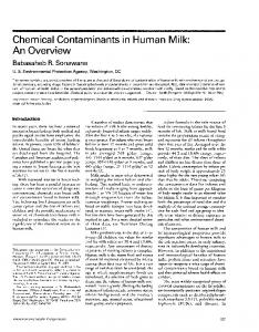
An Overview of Classifier Fusion Methods Dymitr Ruta and Bogdan Gabrys data level fusion, feature level fusion, and classifier fusion [15]. There is little theory about the first two levels of information fusion. However, there have been successful attempts to transform the numerical, interval and linguistic data into a single space of symmetric trapezoidal fuzzy numbers [14], [15], and some heuristic methods have been successfully used for feature level fusion [15]. A number of methods have been developed for classifier fusion also referred to as decision fusion or mixture of experts. Essentially, there are two general groups of classifier fusion techniques. The methods subjectively associated with the first group generally operate on classifiers and put an emphasis on a development of the classifier structure. They do not do anything with classifiers outputs until combination process finds single best classifier or a selected group of classifiers and only then their outputs are taken as a final decision or for further processing [2], [9], [10]. Another group of methods operate mainly on classifiers outputs, and effectively the combination of classifiers outputs is calculated [1], [3]-[8], [11]-[15]. The methods operating on classifiers outputs can be further divided according to the type of the output produced by individual classifiers. A diagrammatic representation of the proposed taxonomy of classifier fusion methods is shown in Figure 1.
A number of classifier fusion methods have been recently developed opening an alternative approach leading to a potential improvement in the classification performance. As there is little theory of information fusion itself, currently we are faced with different methods designed for different problems and producing different results. This paper gives an overview of classifier fusion methods and attempts to identify new trends that may dominate this area of research in future. A taxonomy of fusion methods trying to bring some order into the existing “pudding of diversities” is also provided. 1. INTRODUCTION The objective of all decision support systems (DSS) is to create a model, which given a minimum amount of input data/information, is able to produce correct decisions. Quite often, especially in safety critical systems, the correctness of the decisions taken is of crucial importance. In such cases the minimum information constraint is not that important as long as the derivation of the final decision is obtained in a reasonable time. According to one approach, the progress of DSS should be based on continuous development of existing methods as well as discovering new ones. Another approach suggests that as the limits of the existing individual method are approached and it is hard to develop a better one, the solution of the problem might be just to combine existing well performing methods, hoping that better results will be achieved. Such fusion of information seems to be worth applying in terms of uncertainty reduction. Each of individual methods produces some errors, not mentioning that the input information might be corrupted and incomplete. However, different methods performing on different data should produce different errors, and assuming that all individual methods perform well, combination of such multiple experts should reduce overall classification error and as a consequence emphasise correct outputs. Information fusion techniques have been intensively investigated in recent years and their applicability for classification domain has been widely tested [1]-[14].
�� ����� �� �� ������������� ������������������ Dynamic Classifier Selection
Classifier Structuring and Grouping
Hierarchical Mixtures of Experts
Concepts CF methods operating on classifiers CF methods operating on classifier outputs
No training
Classifier Fusion (CF) System
Class Rankings
Class Labels
Class Set Reduction
Voting Methods
Knowledge-Be haviour Space
Trained
Intersection of Neighbourhoods
Soft / Fuzzy outputs
Class Set Reordering
The Highest Rank
Borda Count
DempsterShaffer Combination Average Bayes Cobmination Product of Experts Fuzzy Integrals Fuzzy Template Neural Network
Union of Neighbourhoods
Logistic Reggresion
From the three possible types of outputs generated by individual classifiers the crisp labels offer the minimum amount of input information for fusion methods, as no information about potential alternatives is available. Some additional useful information can be gained from classification methods generating outputs in a form of class rankings.
The problem arouse naturally as a need of improvement of classification rates obtained from individual classifiers. Fusion of data/information can be carried out on three levels of abstraction closely connected with the flow of the classification process:
1
However, fusion methods operating on classifiers with soft/fuzzy outputs can be expected to produce the greatest improvement in classification performance. The remaining of this paper is organised as follows. In section II methods operating on classifiers are briefly presented. The following three sections provide an overview of the classifier fusion methods operating on single class labels, class rankings and fuzzy measures respectively. Finally conclusions and suggestions for future work are presented.
performing local classifiers. However, applying the DCS method sequentially, excluding the best classifier each time, it is possible to obtain a very reliable ranking of classifiers and eventually also class rankings. Such an approach could be treated as a good pre-processing stage before other methods operating on class rankings are used. 2.2 Classifier Structuring and Grouping Classifiers and their combination functions may be organized in many different ways [2]. The standard approach is to organise them in parallel and simultaneously and separately get their outputs as an input for a combination function or alternatively sequentially apply several combination functions. According to another strategy, a more reasonable approach is to organise all classifiers into groups and to apply different fusion methods for each group. In general, classifiers may be arranged in a multistage structure. At each stage different fusion methods should be applied for different groups of classifiers. Additionally, DCS methods could be used at some stage for selection of the best classifier in each group.
2. METHODS OPERATING ON CLASSIFIERS As mentioned in the introduction, a number of fusion methods operate on the classifiers rather than their outputs, trying to improve the classification rate by pushing classifiers into an optimised structure. Among these methods a dominant role is played by Dynamic Classifier Selection, which is sometimes referred to as an alternative approach to the classifier fusion. The other two approaches reviewed in this section include classifier structuring and grouping and hierarchical mixture of experts. 2.1 Dynamic Classifier Selection
There are a lot of different design options, which are likely to be specific for a particular application. However, at each stage of grouping, a very important factor is the level of diversity of classifier types, training data and methods involved [17]. Any possible classification improvement may only be achieved if the total information uncertainty is reduced [16]. This in turn depends on the diversity of information supporting different classification methods.
Dynamic Classifier Selection (DCS) methods reflect the tendency to extract a single best classifier instead of mixing many different classifiers. DCS attempts to determine a single classifier, which is the most likely to produce the correct classification label for an input sample [2], [10]. As a result only the output of the selected classifier is taken as a final decision. Dynamic classifier selection process includes a partitioning of the input samples. There are a number of methods for the partition forming, starting from the classifiers agreement on the top choices, up to the grouping of features of input samples.
On the other hand, the same goal can be achieved by reduction of errors produced by individual classifiers. Decision combination process tries to minimise the final classification error. As most combination functions work on the basis of increased importance of repetitive inputs, the greater the diversity of the errors produced by individual classifiers, the lower their impact on the final decision and effectively the lower final error. This rule can be applied for any kind of groupings and structuring that might be used in the multiple classifier system.
An example of DCS method is recently developed DCS by Local Accuracy (DCS-LA). Having defined the set of partitions, the best classifier for each partition is locally selected. Considering final classification process, an unknown sample is assigned to a partition, and the output of the best classifier for that partition is taken as a final decision. The idea of using DCS-LA is to estimate each classifier’s accuracy in a local region of feature space and then the final decision is taken as an output from the most locally accurate classifier.
2.3 Hierarchical mixture of experts Hierarchical mixture of experts (HME) is an example of the fusion method, which strength comes from classifiers structure. HME represents a supervised learning technique based on the divide-and-conquer principle, which is broadly used throughout computer science and applied mathematics [9]. The HME is conceptually organised in a tree-like structure of leaves. Each leave represents an individual expert network, which given the input vector x tries to solve local supervised learning problem. The outputs of the
Another approach assumes estimating a local regression model (i.e. logistic regression [2]) for each partition. After the model is estimated for each partition, a relevant decision combination function is selected dynamically for each test case. All DCS methods strongly rely on training data and by choosing only locally best classifier they seem to lose some useful information available from other well 2
elements of the same node are partitioned and combined by the gating network and the total output of the node is given as a convex combination. The expert networks are trained to increase the posterior probability according to Bayes rule and then a number of learning algorithms can be applied to tune the mixture model.
where is a parameter and k(d) is a function that provides additional voting constraints. The most conservative voting rule is given if k(d) = 0 and = 1 , meaning that the class is chosen when all classifiers produce the same output. This rule can be liberalised by lowering the parameter . The case where = 0.5 is commonly known as the majority vote. Function k(d) is usually interpreted as a level of abjection to the most often selected class and refers mainly to the score of the second ranked class. This option allows to adjust the level of collision that is still acceptable for giving correct decision.
Recently the EM algorithm was developed for the HME architecture [9]. The tests on the robot dynamics problem showed a substantial improvement in comparison with the back-propagation neural network. The HME technique does not seem to be applicable for a large dimensional data, as increase of the complexity of the tree-like architecture and associated input space subdivision lead to the increased variance and numerical instability.
3.2 Behaviour-Knowledge Space Method Most fusion methods assume independence of the decisions made by individual classifiers. This is in fact not necessarily true and Behaviour-Knowledge Space method (BKS) does not require this condition [12]. It provides a knowledge space by collecting the records of the decisions of all classifiers for each learned sample. If the decision fusion problem is defined as a mapping of K classifiers: e 1 ,..., e K into M classes: c 1 ,..., c M , the method operates on the K - dimensional space. Each dimension corresponds to an individual classifier, which can produce M + 1 crisp decisions, M class labels and one rejection decision. A unit of BKS is an intersection of decisions of every single classifier. Each BKS unit contains three types of data: the total number of incoming samples: Te ,...,e , the best representative class: R e ,...,e , and the total number of incoming samples for each class: n e ,...,e (m) . In the first stage of BKS method the training data are extensively exploited to build the BKS. Then the final classification decision for an input sample is derived in the focal unit where the balance is estimated between the current classifiers decisions and the recorded behaviour information as shown in the following rule:
3. FUSING SINGLE CLASS LABELS Classifiers producing crisp, single class labels (SCL) provide the least amount of useful information for the combination process. However, they are still well performing classifiers, which could be applied to a variety of real-life problems. If some training data are available, it is possible to upgrade the outputs of these classifiers to the group operating on class rankings or even fuzzy measures. There are a number of methods to achieve this goal, for instance by performing an empirical probability distribution over a set of training data. The two most representative methods for fusing SCL classifiers, namely generalised voting method, and Knowledge-Bahaviour Space method, are now presented.
1
1
K
1
3.1 Voting Methods Voting strategies can be applied to a multiple classifier system assuming that each classifier gives a single class label as an output and no training data are available. There are a number of approaches to combination of such uncertain information units in order to obtain the best final decision. However, they all lead to the generalised voting definition. For convenience let the output of the classifiers form the decision vector d defined as d = [d 1 , d 2 ,..., d n ] T where d i ∈{c1 , c2 ,..., c m , r} , ci denotes the label of the i-th class and r the rejection of assigning the input sample to any class. Let binary characteristic function be defined as follows: 1 if Bj (ci ) = 0 if
if R E(x) = e ,...,e rejection 1
n
1
n e ,...,e (R e ,...,e ) 1
K
K
1
Te ,...,e 1
K
≥
K
otherwise
4. CLASS RANKING BASED TECHNIQUES
d j = ci d j ≠ ci
Among the fusion methods operating on class rankings as the outputs from multiple classifiers, two main approaches are worth mentioning. The first is based on a class set reduction and its objective is to reduce the set of considered classes to as small a number as possible but ensuring that the correct class is still represented in the reduced set. Another
n
∀ ∑ B j (ct ) ≤ ∑ B j (ci ) ≥α ⋅ m + k(d)
t ∈{1,..,m} j =1
Te ,...,e > 0 ∩
K
where is a threshold controlling the reliability of the final decision. The model tuning process should include automatic finding of the threshold .
Then the general voting routine can be defined as: c if E(d) = i r
K
K
j =1
otherwise
3
approach aims at a class set reordering in order to obtain the true class ranked as close to the top as possible. Interestingly, both approaches may be applied to the same problem, so that the set of the classes is first reduced and then reordered.
referring to each class. According to the Highest Rank (HR) method [2], the minimum from these groups of rankings is assigned to each class and then classes are sorted according to the new ranks. If an individual class has to be determined as a final decision, the one from the top of the reordered ranking is chosen. This method is particularly dedicated to cases with a large number of classes and few classifiers. An advantage of the HR method is that it utilises the strength of every single classifier, which means that as long as there is at least one classifier that performs well, the true class should always be near the top of the final ranking. The weakness is that combined ranking may have many ties, which have to be resolved by additional criteria.
4.1 Class Set Reduction Methods At an early stage of combining multiple classifiers, it is reasonable to try to reduce the set of possible classes. Two main criteria have to be taken into consideration while reducing the class set: the size of the set of classes and the probability of containing the true class in the reduced set of classes. The class set reduction (CSR) methods try to find the trade-off between the minimising of the class set and maximising of the probability of inclusion of the true class. Two different approaches are dominant in this type of analysis.
4.2.2 The Borda Count Method Borda Count (BC) is an example of group consensus functions, defined as a mapping from a set of individual rankings to a combined ranking leading to the most relevant decision [1], [2]. For a particular class c k Borda Count B(c k ) is defined as a sum of the number of classes ranked below class c k by each classifier. The magnitude of the BC reflects the level of agreement that the input pattern belongs to the considered class. To a certain degree the BC can be treated as a generalization of the majority-voting rule and for a case of two classes problem it is exactly reduced to the majority vote.
4.1.1 Intersection of Neighbourhoods One CSR method computes an intersection of large neighbourhoods trying to find the threshold rank of a class, below which classes are removed [2]. To achieve this, firstly the neighbourhoods of all classifiers are determined by the ranks of true classes for the worst case in the training data set. The lowest rank ever given by any of the classifier is taken as the threshold and only the classes that are ranked above are used for further processing. This method also recognises redundant classifiers as the ones for which the thresholds are equal to the size of the class set. Intersection approach should only be applied to the classifiers with moderate worst-case performance.
The idea behind the BC method is based on the assumption of additive independence among the contributing classifiers. The method ignores the redundant classifiers, which reinforce errors made by other classifiers. The Borda Count method is easy to implement and does not require any training. Weak point of this technique is that it treats all classifiers equally and does not take into account individual classifiers capabilities. This disadvantage can be reduced to a certain degree by applying weights and calculation of BC as a weighted sum of a number of classes. The weights can be different for every classifier, which in turn requires additional training.
4.1.2 Union of Neighbourhoods Another method provides a union of small neighbourhoods taken from each classifier [2]. The threshold for each classifier is calculated as the maximum (worst) of the minimums (best) of ranks of true classes over the training data set. The redundant classifier can be easily determined, as its threshold equals to zero meaning that its output is always incorrect. This method is suitable for the classifiers with different types of inputs.
4.2.3 Logistic Regression The Borda Count method does not recognise the quality of individual classifiers outputs. An improvement can be achieved by assigning the weights to each classifier reflecting their importance in a multiple decision system and performing so-called logistic regression [2]. An important thing at this stage is to distinguish the classification correctness and classifiers correlation, treating them as separate problems to be modelled. If we assume that the responses: (x 1 , x 2 ,..., x m ) from m classifiers are highest for the classes ranked at the top of the ranking it is possible to use the logistic response function:
4.2 Class Set Reordering Methods Class Set Reordering (CSRR) methods try to improve overall rank of the true class. The CSRR method is considered to be successful if it ranks the true class higher than any individual classifier. Three most commonly used techniques are here presented [2]. 4.2.1 The Highest Rank Method Assuming that each classifier produces a ranking list of classes, it is possible to make groups of rankings 4
�[
=
exp( + 1 x 1 + 2 x 2 + ... + m x m ) 1 + exp( + 1 x 1 + 2 x 2 + ... + m x m )
where i = 1,.., m . Such a Bayes decision, based on the newly estimated posterior probabilities is called an average Bayes classifier. This approach can be applied for the Bayes classifiers. For other classifiers there is a number of methods to estimate posterior probability. As an example for the k – NN classifier the transformation is given in the following form:
� , 2 ,..., m are parameters, which are where 1 constant. The output of the transformation:
L(x) = log
�[
1−
�[
=( +
1
x1 +
2
x 2 + ... +
m
xm )
Pk ( x ∈ C i x ) =
is referred to as logit and provides new value according to which combined rankings are created. The model parameters can be estimated using data fitting methods based on maximum likelihood. The logits or �[ values can be additionally treated as confidence measures. It is possible to determine a threshold value so that classes with confidence value below the threshold are rejected. 5. SOFT-OUTPUT METHODS
CLASSIFIER
where k i denotes the number of prototype samples from class C i out of all k nn nearest prototype samples. The quality of the Bayes average classifier depends on how the posterior probabilities are estimated and the diversity of used classifiers. 5.1.2 Bayes Belief Integration
FUSION
The approach mentioned above treats equally all the classifiers and does not explicitly consider different errors produced by each of them. These errors can be comprehensively described by means of confusion matrix given by:
The largest group of classifier fusion methods operate on classifiers which produce so-called soft outputs. The outputs are the real values in the range [0,1] . These values are generally referred to as fuzzy measures, which cover all known measures of evidence: probability, possibility, necessity, belief and plausibility [16]. All these measures are used to describe different dimensions of information uncertainty. Effectively, the fusion methods in this group try to reduce the level of uncertainty maximising suitable measures of evidence.
n 11 (k ) PTk = ... (k ) n M1
The Bayesian methods can be applied to the classifier fusion under the condition that the outputs of the classifier are expressed in posterior probabilities. Effectively combination of given likelihoods is also a probability of the same type, which is expected to be higher than the probability of the best individual classifier for the correct class. Two basic Bayesian fusion methods are introduced. The first one named Bayes Average is a simple average of posterior probabilities. The second method uses Bayesian methodology to provide a belief measure associated with each classifier output and eventually integrates all single beliefs resulting in a combined final belief.
n 1 ( M +1 )
Bel( x ∈ c i e k ( x )) = P( x ∈ c i e k ( x ) = j k ) j = 1,..., M + 1 and
where i = 1,..., M ;
P( x ∈ c i e k (x) = j) =
n ij M
(k )
∑ n ij
(k )
i =1
Having defined such a belief measure for each classifier we can combine them in order to create new belief measure of the multiple classifier system as follows:
5.1.1 Simple Bayes Average If the outputs of the multiple classifier system are given as posterior probabilities that an input sample x comes from a particular class Ci , i = 1,.., m : P(x ∈ Ci x) , it is possible to calculate an average posterior probability taken from all classifiers: 1 K
(k )
... ... (k ) ... n M ( M +1) ...
where rows correspond to classes: c 1 ,..., c M from which the input sample was drawn from and columns denote the classes to which the input sample was assigned by the classifier e k . The values n i, j ( k ) express how many input samples coming from class c i were assigned to class c j . On the basis of the confusion matrix PTk it is possible to build the belief measure of correct assignment as given by:
5.1 Bayesian Fusion Methods
PE ( x ∈ C i x ) =
ki k nn
∏k =1 P( x ∈ c i e k (x) = j k ) K ∏ k =1 P(x ∈ c i ) K
Bel(i) = P(x ∈ c i )
The probabilities used in the above formula can be easily estimated from the confusion matrix. The class
K
∑ PK ( x ∈ C i x ) k =1
5
where A i = {x 1 ,..., x i } . Note that when g is the fuzzy measure, the values of g(A i ) can be computed recursively as:
with the highest combined belief measure: Bel(i) is chosen as a final classification decision. Alternatively selection of any class may be rejected if the combined belief is smaller than a specified threshold value.
g(A 1 ) = g({x 1 }) = g 1 g(A i ) = g i + g(A i −1 ) +
5.2 Fuzzy Integrals Fuzzy integrals aim at searching for the maximal agreement between the real possibilities relating to objective evidence and the expectation g which defines the level of importance of a subset of sources. The concept of fuzzy integrals arises from the -fuzzy measure g developed by Sugeno. It generalises the probability by adding parameter to the additive probability measure with respect to disjoint objects of measure: ∀ g(A ∪ B) = g(A) + g(B) +
A, B ⊂ X A∩B=0
n
J
i
i
g(A i −1 )
for 1 < i ≤ n
For pattern recognition applications, the function h k ( x i ) can be treated as a partial evaluation of the degree of belonging of the object A to class k , given by the classifier associated with a group of features x i . Sugeno integral can be successfully applied to any multi-sensor systems by fusing the classifiers outputs in order to provide more accurate classification rates. 5.2.2 Choquet Fuzzy Integral
J�$ J�%
Choquet fuzzy integral, developed by Sugeno and Murofushi, provides an extension to the Lebesgue integral which Sugeno integral do not cover. The definition of the Choquet integral refers to the Choquet functional presented in a different context. The assumptions are the same as for the Sugeno integral. The Choquet integral over set A ⊆ of the function h : X → [0,1] with respect to a fuzzy measure g is defined by:
From the normalization g(X) = 1 we can derive value by solving the equation: + 1 = ∏ (1 +
J
)
i =1
where g i are fuzzy densities which could be chosen subjectively or estimated through a training process. Thus, knowing the fuzzy densities g i , i = 1,..., n , one can construct the fuzzy measure g for the set A . The fuzzy measures g are a subclass of belief (for ≥ 0 ) and plausibility (for ≤ 0 ) measures defined by Shafer.
+∞
∫A h(x) o g(⋅) = ∫0 g(A )d where A = {x | h(x) > } . Calculation of the Choquet fuzzy integral is similar to the numerical methods of integral calculation: n
e = ∑ [h(x i ) − h(x i −1 )]g in
5.2.1 Sugeno Fuzzy Integral
i =1
Sugeno fuzzy integral combines objective evidence of an hypothesis with the prior expectation of the importance of the evidence to the hypothesis. If we introduce a measurable space (X, Ω) and a function h : X → [0,1] then the fuzzy integral over set A ⊆ of the function h with respect to a fuzzy measure g is defined by:
where h(x 0 ) = 0 and g ij = g({x i , x i +1 ,..., x j }) . The Choquet integral reduces to the Lebesque integral for a probability measure when a probability density function is used for calculations. Comparative results from the fusion of handwritten word classifiers showed similar level of classification performance for both integrals.
[min( min h(x), g(A ∩ E))] ∫A h(x) o g(⋅) = sup X∈E E⊆X
5.2.3 Weber Fuzzy Integral Weber fuzzy integral is a result of an attempt to improve the quality of fuzzy integrals based on the Sugeno fuzzy measure. Weber originally proposed a generalisation of the Sugeno integral and Keller and Tahani have extended this approach introducing a large family of measures called S -decomposable measures. Given a triangular co-norm S , the S decomposable measure g has the property: g(A ∪ B) = S(g(A), g(B)) if A ∩ B = 0 . The possibility measure is an example of such a measure with S
Calculation of the Sugeno fuzzy integral is unexpectedly easy if we reorder elements of a set X = {x 1 ,..., x n } so that the condition: h ( x 1 ) ≥ h ( x 2 ) ≥ ... ≥ h ( x n ) is met. Then a fuzzy integral e with respect to the fuzzy measure g over X can be computed by: n
e = max[min(h(x i ), g(A i ))] i =1
6
measures of an uncertain belief that given proposition is true or is not true respectively. Only non-rejecting classifiers are taken into account for the combination. Also classifiers with the substitution rate equal (k ) = 1 should be removed from the system. If there ss
being the maximum operator. With the above property, a set of information sources can be obtained after the fuzzy densities are determined. An example of the t-conorm is: S p (a, b) = (a p + b p − a p b p ) 1 p . Combining the S -decomposable measure with a tconorm, the generalised fuzzy integral is defined as follows:
is one classifier with the recognition rate r (k ) = 1 , it means that it classifies all input samples with absolute certainty and other classifiers are no longer needed. In a general case the classifier rates are in the range (0,1) and for such classifiers the combination is calculated according to the combination rule:
e T = U[T(h(x i ), g({x 1 ,..., x n }))] i
A number of t-conorms have been tested with respect to their applicability for information fusion. The use of some of them has resulted in a significant increase of the classification performance.
m(A) = m 1 ⊕ m 2 (A) = k
5.3 Dempster-Shaffer Combination
where k −1 = 1 −
According to the Dempster-Shaffer theory the universe consists of exhaustive and mutually exclusive logical statements called propositions: A i ⊂ , i = 1,..., M . Each proposition is assigned a belief value from the range [0,1] , which is based on the presence of evidence e . The value of belief is derived from basic probability assignment (BPA) m(A i ) , i = 1,..., M , which defines an individual impact of each item of evidence on the subsets of the universal set: . If a subset A is given as a disjunction of all elements in A , the belief value of the subset A is given by:
∑! m 1 (X)m 2 (Y) = X∩Y=0
(k )
BmE (A j′ ) + CmE ( k 1 − mE (A j′ ) bel(Aj′ ) = BmE (A j′ ) 1 − mE (A j′ ) k
k
k
k
k
k
m E (A j′ )
p
A=∑
k =1
k
k
k
k
1 − m E (A j′ )
k =1
k
p
, B = ∏ [1 − m E (A j′ )] , k =1
k
k
k
k
k
(1 + A)B
if
p=M p