a validation experiment has been run, using a new random seed for ... Obviously, the validation data ..... The authors are also in debt with Miguel Sánchez.
Comparison of classifier fusion methods for classification in pattern recognition tasks Francisco Moreno-Seco, Jos´e M. I˜ nesta, Pedro J. Ponce de Le´on, and Luisa Mic´o Department of Software and Computing Systems University of Alicante P.O. box 99, E-03080 Alicante, Spain {paco,inesta,pierre,mico}@dlsi.ua.es http://grfia.dlsi.ua.es
Abstract. This work presents a comparison of current research in the use of voting ensembles of classifiers in order to improve the accuracy of single classifiers and make the performance more robust against the difficulties that each individual classifier may have. Also, a number of combination rules are proposed. Different voting schemes are discussed and compared in order to study the performance of the ensemble in each task. The ensembles have been trained on real data available for benchmarking and also applied to a case study related to statistical description models of melodies for music genre recognition.
1
Introduction
Combining classifiers is one of the most widely explored methods in pattern recognition in the recent years. These techniques have been shown to reduce the error rate in classification tasks in opossite to single classifiers. Also, the combination of different techniques to make a final decision makes the performance of the system more robust against the difficulties that each individual classifier may have on each particular data set. Different reasons have been argued for this behaviour, amongst others, statistical, computational or representational reasons [1]. Several different approaches have been used to obtain classifier ensembles. As stated in a recent work by Duin [2], base classifiers should be different, but they should be comparable as well. Also, works on this subject point out the importance of the concept of diversity in classifier ensembles, with respect to both classifier outputs and structure [3–6]. This points out that a trade-off between comparability and diversity is desirable when combining different classifiers. Classifiers for an ensemble can be generated using different initializations (like in neural networks), different parameter choices (like the number of neighbors in the k-NN rule), different classification schemes or, for example, different training sets from the same target problem. A set of classifiers generated in one of these ways is called to be consistent.
2
In this work, the base classifiers used to combine are comparable in terms that they are applied to the same data sets and using the same partitioning, and are diverse since they come from different pattern recognition paradigms: a k-nearest-neighbor (k-NN), a multi-layer perceptron (MLP), a support vector machine (SVM), a decision tree (DT), and a na¨ıve Bayes classifier (NB). All the base classifiers have been trained in the same feature spaces and with the same training set. Current research and new proposals on the decision combination of the base classifiers is presented in this paper. First, the classification techniques based on them are described, along with the different ensemble schemes for combining classifier decisions. Following this, the results for the ensembles are presented and compared with single classifier results for data sets from the UCI/Statlog project [7], and for a data set based on the classification of music styles using MIDI files. Finally, the conclusions drawn from the results are discussed, pointing the research to further work lines.
2
Base classifiers
Five conceptually different classification techniques have been used in this work: the k-nearest-neighbour classifier (k-NN), the naive Bayesian classifier (NB), a support vector machine (SVM), a multi-layer perceptron (MLP), and a decision tree (DT). For the first case, given a sample xi , the distances to the prototypes in the training set are computed, and the class labels of the closest k are taken into account to classify the sample into the most frequent class among them. After some initial testing on the performance of this particular classifier on some of the utilized datasets, a single value k = 3 was established for this classifier in all the experiments for simplicity. The rest of the classifiers have been applied using the default parameters established for them in the open source software project WEKA, using the Explorer interface [8]. The decision tree is the J48. Each base classifier has been trained using the same training set, and its accuracy has been estimated using the same test set. Two methods have been used to train the classifiers, and the ensembles: first, for the UCI/Statlog project data sets, a total of 50 pairs of train/test sets were generated, using 10 random seeds for generating 5 cross-validation pairs (with approximately an 80% of the data for training, and the rest for testing). The base classifiers have been run 50 times with different train and test sets from the same data (each data sample has been classified 10 times). The error rate of the classifier has been estimated by counting the total number of errors over the 50 experiments, divided by the total number of samples classified (that is 10 times the size of the data set). Once the ensembles have been trained with the UCI/Statlog project data sets, a validation experiment has been run, using a new random seed for generating another 5 pairs of train/test sets. The base classifiers have also been run with the validation data, in order to obtain a reference. Obviously, the validation data is not unseen data for the classifiers, as it should be, but the results can be a reference for future experiments on completely unseen data.
3
The training of the base classifiers in the music genre classification task was made under a more realistic approach: each data set has been divided into 5 subsets with approximately the same size. The division has been made at the level of MIDI files. Given the 5 subsets, 3 of them have been used to train the classifier, 1 for test (and for training the ensembles), and the last one for validation. The partitions have been rotated 5 times, in order to obtain more significant results.
3
Ensemble design: voting schemes
Designing a suitable method of decision combinations is a key point for the ensemble’s performance. In this paper, different possibilities have been explored and compared. In particular, several weighted voting methods, along with the unweighted plurality vote (the most frequent class is the winner class). In the discussion that follows, N stands for the number of samples, contained in the M training set X = {x}N i=1 , M is the number of classes in a set C = {cj }j=1 , and K classifiers, Ck , are utilized. a
a
k
1
k
a k
1
1
0 0
N(1−1/M) e k
e
B
e
W
e
k
e
B
e
W
e
k
Fig. 1. Different models for giving the authority (ak ) to each classifier in the ensemble as a function of the number of errors (ek ) made on the training set.
3.1
Unweighted methods
1. Plurality vote (PV). Is the simplest method. Just count the number of decisions for each class and assign the sample xi to the class cj that obtained the highest number of votes. The problem here is that all the classifiers have the same ‘authority’ regardless of their respective abilities to classify properly. In terms of weights it can be considered that wk = 1/K ∀k. 3.2
Weighted methods
2. Simple weighted vote (SWV). The decision of each classifier, Ck , is weighted according to its estimated accuracy (the proportion of successful classifications,
4
αk ) on the training set [9]. This way, the authority for Ck is just ak = αk . Then, its weight wk is: ak (1) wk = P l al Also for the rest of weighting schemes presented here (except the last one), the weights are the normalized values for ak , as shown in this equation. The weak point of this scheme is that an accuracy of 0.5 in a two-class problem still has a fair weight although the classifier is actually unable to predict anything useful. This scheme has been used in other works [10] where the number of classes is rather high. In those conditions this drawback may not be evident. 3. Re-scaled weighted vote (RSWV). The idea is to assign a zero weight to classifiers that only give N/M or less correct decisions on the training set, and scale the weight values proportionally. As a consequence, classifiers with an estimated accuracy αk ≤ 1/M are actually removed from the ensemble. The values for the authority are computed according to the line displayed in figure 1-left. Thus, if ek is the number of errors made by Ck , then ak = max{0, 1 −
M · ek } N · (M − 1)
4. Best-worst weighted vote (BWWV). In this ensemble, the best and the worst classifiers in the ensemble are identified using their estimated accuracy. A maximum authority, ak = 1, is assigned to the former and a null one, ak = 0, to the latter, being equivalent to remove this classifier from the ensemble. The rest of classifiers are rated linearly between these extremes (see figure 1-center). The values for ak are calculated as follows: ak = 1 −
ek − eB eW − eB
,
where eB = min{ek } k
and eW = max{ek } k
5. Quadratic best-worst weighted vote (QBWWV). In order to give more authority to the opinions given by the most accurate classifiers, the values obtained by the former approach are squared (see figure 1-right). This way, ak = (
eW − ek 2 ) eW − eB
.
6. Weighted majority vote (WMV) The theorem 4.1 of Kuncheva’s book [11, p. 124] states that accuracy of the ensemble is maximized by assigning weights wk ∝ log
αk 1 − αk
5
where αk is the individual accuracy of the classifier. In order to use a voting method of this type as a reference for the previously proposed methods (numbers 3 to 5), in this case the weight of each classifier is computed as: αk wk = log 1 − αk Classification by the weighted methods. Once the weights for each classifier decision have been computed, the class receiving the highest score in the voting is the final class prediction. If cˆk (xi ) is the prediction of Ck for the sample xi , then the prediction of the ensemble can be computed as X wk δ(ˆ ck (xi ), cj ) , (2) cˆ(x) = arg max cj ∈C
k
being δ(a, b) = 1 if a = b and 0 otherwise. Since thePweights represent the normalized authority of each classifier, it M follows that k=1 wk = 1. This makes it possible to interpret the sum in Eq. 2 as P (xi |cj ), the probability that xi is classified into cj .
4
Experiments
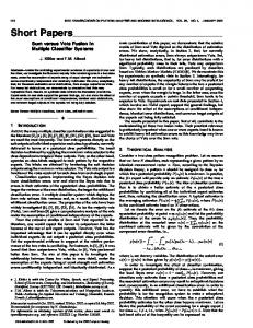
Two different experiments have been carried out in order to compare the voting schemes proposed (numbers 3 to 5) with those of reference (1, 2 and 6). The first experiment tries to study the performance of the voting schemes when used with benchmarking data. For that, 19 data sets from the public available UCI/Statlog projects have been utilized. Each data set has been partitioned as explained in section 2. In total, 50 pairs of train/test sets were generated, so a total number of 50 experiments for each data set have been run in order to train the weights of the ensembles. The error rates of each base classifier were computed as the total number of errors made (on the 50 experiments) divided by the total number of samples classified. Finally, in order to test the ensembles, another 5 pairs of train/test sets were generated for validation. Recall from section 2 that the validation data are not unseen data. The table 1 presents the error rates of the validation experiments for the datasets, with the best results for each data set emphasized in boldface. Note that the result for the best single classifier classifier is showed as a reference. To summarize the results, the ensembles outperform the best classifier in 8 out of 19 data sets, the best classifier wins in 5 data sets, and in the remaining 6 data sets they obtain the same error rate. Specially significant is the result for the glass database, where the ensembles obtain an error rate which is almost 4% below the error rate of the best classifier. Note that the quadratic best-worst has performed the best, being 8 times one of the winner schemes. Note that the best single classifier was not always the same (1 NB, 1 SVM, and 3 MLP) and there are not analytic methods to decide which is the best classifier to be used according to the data. Thus, the ensembles seem a better option for designing a classification system.
6 Data set australian balance cancer diabetes german glass heart ionosphere liver monkey1 phoneme segmen sonar vehicle vote vowel waveform21 waveform40 wine
PV 13.04 12.64 3.37 23.18 24.30 32.71 15.93 9.12 36.81 3.60 16.78 3.51 24.04 21.75 4.37 14.02 14.74 14.50 1.69
SWV RSWV BWWV QBWWV WMV 13.04 13.04 13.62 14.64 13.04 11.36 11.36 10.56 10.56 11.20 3.37 3.37 3.37 3.37 3.37 23.18 23.18 23.44 22.66 23.18 24.30 24.30 23.5 23.70 24.30 30.84 30.84 28.51 29.91 28.51 15.93 15.93 15.19 15.19 15.93 9.12 9.12 11.11 11.11 9.12 36.81 35.36 33.62 31.88 35.36 3.60 0 0 0 0 16.78 16.78 13.53 12.31 16.78 3.07 3.07 2.55 2.55 3.07 24.04 24.04 23.08 23.08 24.04 21.04 21.04 20.33 20.33 20.33 4.37 4.37 3.69 4.14 4.37 11.74 11.74 5.87 4.92 5.68 14.70 14.70 13.36 13.3 14.70 14.50 14.50 13.96 13.74 14.50 1.69 1.69 2.25 2.25 1.69
Best 14.64 (SVM) 8.80 (MLP) 3.22 (SVM) 22.66 (SVM) 23.70 (SVM) 32.24 (MLP) 14.07 (NB) 9.40 (MLP) 31.88 (MLP) 0 (MLP) 12.31 (3-NN) 3.77 (DT) 22.12 (MLP) 18.91 (MLP) 4.14 (DT) 4.92 (3-NN) 13.30 (SVM) 13.74 (SVM) 1.69 (NB)
Table 1. Error rates (in %) of the different ensembles with the UCI/Statlog data sets, together with the result of the best individual classifier (Best) column. The winning classifications schemes in terms of accuracy for each data set have been highlighted.
A case study. In order to test on a real new problem the experiences we have learned from the first study, the same approach is now applied to a real problem related to music information retrieval. The goal is to classify a digital music score into a set of genres. In this case, jazz and classical music have been consider due to a general agreement among the experts about their definitions and taxonomy. The JvC (Jazz vs. Classical) corpus is made up of samples extracted from standard MIDI files1 files from jazz and classical music and it has been already utilized in former works2 [12, 13]. MIDI files contain music in symbolic format (a sort of digital score). The files used here contain a melody track from which descriptors are extracted. All melodies are monophonic sequences of notes (at most one note is playing at any time). The corpus is composed of a total of 150 MIDI files, 65 of them being classical music and 85 being jazz. This dataset represents more than 8 hours of music. Each sample is a vector of musical descriptors for a number of feature categories that assess melodic, harmonic and rhythmic properties of a melody. These descriptors are mainly descriptive statistics like, for example, average note pitch, 1 2
http://www.midi.org This dataset is available for research purposes on request to the authors.
7
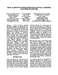
standard deviation of note durations, pitch interval range, etc. A total of 28 descriptors are available. From the set of MIDI files two datasets have been built. The first one composed of 150 samples, one sample per melody track. The second one is made up of 7125 samples. For this second dataset, each sample corresponds to a fragment of a melody, extracted applying a 50-bar wide sliding window on each melody track. The window is shifted one bar at each time along the track, until the end of the track is reached. Each time the window is shifted, a new sample is extracted. Being ω the size of the window, the first dataset corresponds to a value ω = ∞, and the second dataset for ω = 50. The experiments with the JvC data sets have been carried out using a train, test, and validation scheme. Random partitions are not advisable since for ω = 50 attention has to be paid to samples belonging to the same melody do not appear in both training and test or validation. This fact would underestimate the error estimation. Each data set has been splitted into 5 partitions (keeping in the same partition those samples belonging to the same MIDI file). 3 of them have been used for training, 1 for test, and the remaining one for validation. The experiment has been repeated 5 times, rotating the partitions. The results of the validation presented in table 2 are average error rates from the 5 experiments. Ensemble/classifier Plurality SWV RSWV BWWV QBWWV WMV 3-NN DT MLP NB SVM
Data set JvC, ω = ∞ JvC, ω = 50 7.33 9.28 7.33 9.28 7.33 9.16 6.00 6.31 6.00 8.29 6.00 9.46 6.00 11.80 13.33 15.66 8.00 13.30 16.00 15.56 10.67 11.08
Table 2. Average error rates (in %) of the different ensembles with the JvC data sets, together with the results of the base classifiers.
The results for ω = ∞ show that even when the best single classifier (the 3-NN classifier) is much better than all the other single classifiers, the ensembles still perform adequately. For the ω = 50 data set, the ensembles perform much better than any base classifier, specially the BWWV, which obtains an error rate 4.5% below the rate of the best classifier (SVM). The results shown in table 2 confirm that the ensembles performance is better in the general case (although in some cases may be slightly worse than a single particular classifier).
8
5
Conclusions
We have proposed three weighted voting methods (RSWV, BWWV, and QBWWV) for classifier ensembles, and we have tested their performance with the UCI/Statlog project data sets (a widely known repository of real data sets), and also with a case study of music genre classification. In both cases the proposed ensembles have shown a more robust performance in general than individual classifiers, and with some data sets the results of the best ensemble is much better than that of a classifier. Among all the voting schemes tested, the approaches based on scaling the weights to a range established by the best and the worst classifiers have shown the best classification accuracy in most of the data sets. Future work includes a more adequate validation scheme for the UCI/Statlog project data sets, and using more base classifiers for testing the ensembles. Also, we plan to study more carefully the results of each ensemble on the data sets to find out the reasons of the (good or bad) performance of the ensemble, and develop new voting methods to improve these results.
Acknowledgments The authors wish to thank Roberto Paredes from the Politechnical University of Valencia for providing us with the UCI/Statlog data sets, and the program for generating the partitions. The authors are also in debt with Miguel S´anchez Molina from University of Alicante, for his valuable help with the WEKA tool. This work was supported by the Spanish project CICyT TIC2003–08496–C04, the project GV06/166 from Generalitat Valenciana, and the IST Programme of the European Community, undes the Pascal Network of Excellence, IST-2002506778.
References 1. Dietterich, T.G.: Ensemble methods in machine learning. Lecture Notes in Computer Science 1857 (2000) 1–15 2. Duin, R.: The combining classifier: to train or not to train? In: Proceedings of the International Conference on Pattern Recognition ICPR’2002. Volume II., Quebec (Canada) (2002) 765–770 3. Dietterich, T.: Ensemble methods in machine learning. In: First Internacional Workshop on Multiple Classifier Systems. (2000) 1–15 4. Kuncheva, L.I.: That elusive diversity in classifier ensembles. In: Proc. 1st Iberian Conf. on Pattern Recognition and Image Analysis (IbPRIA’03). Volume 2652 of Lecture Notes in Computer Science. (2003) 1126–1138 5. Kuncheva, L.I., Whitaker, C.J.: Measures of diversity in classifier ensembles. Machine Learning 51 (2003) 181–207 6. Partridge, D., Griffith, N.: Multiple classifier systems: Software engineered, automatically modular leading to a taxonomic overview. Pattern Analysis and Applications 5 (2002) 180–188
9 7. Blake, C., Merz, C.: UCI repository of machine learning databases (1998) 8. Witten, I., Frank, E.: Data Mining: Practical machine learning tools and techniques. 2nd edn. Morgan Kaufmann, San Francisco (USA) (2005) 9. Opitz, D., Shavlik, J.: Generating accurate and diverse members of a neuralnetwork ensemble. In Touretzky, D., Mozer, M., Hasselmo, M., eds.: Advances in Neural Information Processing Systems. Volume 8. (1996) 535–541 10. Stamatatos, E., Widmer, G.: Music performer recognition using an ensemble of simple classifiers. In: Proceedings of the European Conference on Artificial Intelligence (ECAI). (2002) 335–339 11. Kuncheva, L.: Combining Pattern Classifiers: methods and algorithms. Wiley (2004) 12. Ponce de Le´ on, P.J., I˜ nesta, J.M.: Statistical description models for melody analysis and characterization. In: Proceedings of the 2004 International Computer Music Conference, International Computer Music Association (2004) 149–156 13. P´erez-Sancho, C., I˜ nesta, J.M., Calera-Rubio, J.: Style recognition through statistical event models. In: Proceedings of the Sound and Music Computing Conference, SMC’04. (2004)