Nov 5, 2002 - Traditional ad-hoc testing of software systems still seems to be the main ... 7, 8], a high-performance system supporting both rewriting logic and ...
An Overview of the Runtime Verification Tool Java PathExplorer Klaus Havelund Kestrel Technology NASA Ames Research Center
Grigore Ro¸su Department of Computer Science University of Illinois at Urbana-Champaign
http://ase.arc.nasa.gov/havelund
http://cs.uiuc.edu/grosu
November 5, 2002
Abstract We present an overview of the Java PathExplorer runtime verification tool, in short referred to as JPaX. JPaX can monitor the execution of a Java program and check that it conforms with a set of user provided properties formulated in temporal logic. JPaX can in addition analyze the program for concurrency errors such as deadlocks and data races. The concurrency analysis requires no user provided specification. The tool facilitates automated instrumentation of a program’s bytecode, which when executed will emit an event stream, the execution trace, to an observer. The observer dispatches the incoming event stream to a set of observer processes, each performing a specialized analysis, such as the temporal logic verification, the deadlock analysis and the data race analysis. Temporal logic specifications can be formulated by the user in the Maude rewriting logic, where Maude is a high-speed rewriting system for equational logic, but here extended with executable temporal logic. The Maude rewriting engine is then activated as an event driven monitoring process. Alternatively, temporal specifications can be translated into efficient automata, which check the event stream. JPaX can be used during program testing to gain increased information about program executions, and can potentially furthermore be applied during operation to survey safety critical systems.
1
Introduction
Correctness of software is becoming an increasingly important issue in many branches of our society. This is not the least true for NASA’s space agencies, where space craft, rover and avionics technology must satisfy very high safety standards. Recent space mission failures have even further emphasized this. Traditional ad-hoc testing of software systems still seems to be the main approach to achieve higher confidence in software. By traditional testing we mean some manual, and at best systematic, way of generating test cases and some manual, ad-hoc way of evaluating the results of running the test cases. Since evaluating test case executions manually is time consuming, it becomes hard to run large collections of test cases in an automated fashion, for example overnight. Hence, there is a need for generating test oracles in an easy and automated manner, preferably from high level specifications. Furthermore, it is naive to believe that all errors in a software system can be detected before deployment. Hence, one can argue for an additional need to use the test oracles for monitoring the program during execution. This paper presents a system, called Java PathExplorer, or JPaX for short, that can monitor the execution of Java programs, and check that they conform with user provided high level temporal logic specifications. In addition, JPaX analyzes programs for 1
concurrency errors, such as deadlocks and data races, also by analyzing single program executions. The algorithms presented all take as input an execution trace, being a sequence of events relevant for the analysis. An execution trace is obtained by running an instrumented version of the program. Only the instrumentation needs to be modified in case programs in other languages than Java need to be monitored. The analysis algorithms can be re-used. A case study of 35,000 lines of C++ code for a rover controller has for example been carried out, leading to the detection of a deadlock with a minimal amount of effort. Concerning the first form of analysis, temporal logic verification, we consider two forms of logic: future time logic and past time logic. We first show how these can be implemented in Maude [6, 7, 8], a high-performance system supporting both rewriting logic and membership equational logic. The logics are implemented by providing their syntax in Maude’s very convenient mixfix operator notation, and by giving an operational semantics of the temporal operators. The implementation is extremely efficient. The current version of Maude can do up to 3 million rewritings per second on 800Mhz processors, and its compiled version is intended to support 15 million rewritings per second. The Maude rewriting engine is used as an event driven monitoring process, performing the event analysis. The implementation of both these logics in Maude together with a module that handles propositional logic covers less than 130 lines. Therefore, defining new logics should be very feasible for advanced users. Second, we show how one from a specification written in temporal logic (be it future time or past time) can generate an observer automaton that checks the validity of the specification on an execution trace. Such observer automata can be more efficient than the rewriting-based implementations mentioned above. It especially removes the need for running Maude as part of the monitoring environment. Concerning the second form of analysis, concurrency analysis, multi-threaded software is the source of a particular class of transient errors, namely deadlocks and data races. These errors can be very hard to find using standard testing techniques since multi-threaded programs are typically non-deterministic, and the deadlocks and data races are therefore only exposed in certain ”unlucky” executions. Model checking can be used to detect such problems, and basically works by trying all possible executions of the program. Several systems have been developed recently, that can model check software, for example the Java PathFinder system (JPF) developed at NASA Ames Research Center [18, 35], and similar systems [14, 25, 34, 10, 3]. This can, however, be very time and memory consuming (often program states are stored during execution and used to determine whether a state has been already examined before). JPaX contains specialized trace analysis algorithms for deadlock and data race analysis, that from a single random execution trace try to conclude the presence or the absence of deadlocks and data races in other traces of the program. These algorithms, including the Eraser algorithm [33], are based on the derivation of testable properties that are stronger than the original properties of deadlock freedom and data race freedom, but therefore also easier to test. That is, if the program contains a deadlock or a data race then the likelihood of these algorithms to find the problem is much higher than the likelihood of actually meeting the deadlock or data race during execution. The idea of detailed trace analysis is not new. Beyond being the foundation of traditional testing, also more sophisticated trace analysis systems exist. Temporal logic has for example been pursued in the commercial Temporal Rover tool (TR) [11], and in the MaC tool [27]. TR allows the user to specify future time and past time temporal formulae, but requires the user to manually instrument the code. The MaC tool is closer in spirit to what we describe in this paper, except that its specification language is fixed. Neither of these tools provides support for concurrency
2
analysis. A tool like Visual Threads [15, 33] contains hardwired deadlock and data race analysis algorithms, but only works on Compaq platforms and only on C and C++. Furthermore, Visual Threads cannot be easily extended by a user, while JPaX can. We furthermore have improved the deadlock analysis algorithm to yield fewer false positives, an important objective if one wants such a tool to be adopted by programmers. For an overview of recent work in runtime verification we refer the reader to the proceedings of RV’01 and RV’02, the 1st and 2nd workshops on runtime verification [1, 2]. This paper is a summary of several papers written on Java PathExplorer [22, 21, 20, 17, 24, 23, 4, 16, 32, 19]. A rewriting implementation for future time LTL is presented in [22] and [23]. A rewriting implementation of past time LTL is presented in [21]. Generation of observer automata for future time LTL is described in [23]. Generation of observer dynamic programming algorithms for past time LTL is presented in [24]. Concurrency analysis is studied in [4] and [16]. In [13] a framework is described for translating future time LTL to Buchi-like automata. The paper is organized as follows. Section 2 gives an overview of the JPaX system architecture. Section 3 introduces the temporal logics that have been implemented in JPaX, namely future time and past time temporal logic. Each logic is defined by its syntax and its semantics. Section 4 presents the various algorithms for monitoring the logics. First (Subsection 4.1) the rewriting based approach is presented, showing how future time and past time logic can be encoded in the Maude rewriting system, and how Maude is then used as the monitoring engine. Second (Subsection 4.2) the observer automata/algorithm approach is presented, showing how efficient observer automata and algorithms can be generated from future time respectively past time temporal logic. Section 5 presents the concurrency analysis algorithms for detecting respectively data races and deadlocks. Finally, Section 6 concludes the paper.
2
Architecture of JPaX
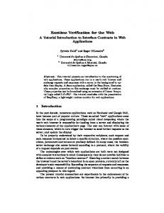
Java PathExplorer (JPaX ) is a system for monitoring the execution of Java programs. The system extracts an execution trace from a running program and verifies that the trace satisfies certain properties. An execution trace is a sequence of events, of which there are several kinds as we shall discuss below. Two forms of monitoring are supported: temporal verification and concurrency analysis. In temporal verification the user provides a specification in temporal logic of how the observed system is expected to behave. The models of this specification are all the execution traces that satisfy it. Finite execution traces generated by running the program are checked against the specification for model conformance, and error messages are issued in case of failure. In concurrency analysis, we are analyzing the trace for symptoms of concurrency problems, such as deadlocks and data races. JPaX itself is written in Java and consists of an instrumentation module and an observer module, see Figure 1. The instrumentation module automatically instruments the bytecode class files of a compiled program by adding new instructions that when executed generate the execution trace. The Java bytecode instrumentation is performed using the Jtrek Java bytecode engineering tool [9]. Jtrek makes it possible to easily read Java class files (bytecode files), and traverse them as abstract syntax trees while examining their contents, and insert new code. The inserted code can access the contents of various runtime data structures, such as for example the call-time stack, and will, when eventually executed, emit events carrying this extracted information to the observer. Six kinds of events are generated: write(t, x) (thread t writes to variable x), read(t, x) (thread t reads 3
Specifications Instrumentation
Verification
Java Program
Observer Deadlock
Bytecode
Dispatcher
Event Stream
Compile
Datarace LTL
Maude
Instrument ... Instrumented Bytecode
Execute (JVM)
Figure 1: Overview of JPaX variable x), lock(t, o) (thread t locks object o), unlock(t, o) (thread t unlocks object o), start(t 1 , t2 ) (thread t1 starts thread t2 ), join(t1 , t2 ) (thread t1 joins thread t2 ). The events (trace) are either written to a file or to a socket, in both cases in plain text format. The observer will read the events correspondingly. In case sockets are used, the observer can run in parallel with the observed program, even on a different computer, and perform the analysis in real time. An instrumentation script guides the instrumentation by stating which events should be reported in the execution traces. For concurrency analysis this simply amounts to identifying whether deadlock analysis or data race analysis is desired. Data race analysis is the most comprehensive instrumentation and requires all above events to be generated, while deadlock analysis requires all except write and read events. Temporal verification only requires the generation of write events for those variables that influence the evaluation of the user provided temporal formulae. In this case the script identifies explicitly these variables, together with a set of observable named predicates over these variables. Only the observable predicates can be referred to (by name) in the temporal properties. The advantage of this layered approach, as also stated in [27], is that the requirement specification can be created without considering low level issues (such as what variables exist in the program), and can even be created before the construction of the program as part of the systems requirements. The observer module is responsible for performing the trace analysis. It receives the events and dispatches these to a set of observer rules, each rule performing a particular analysis that has been requested. Generally, this modular rule based design allows a user to easily define new runtime verification procedures without interfering with legacy code. Observer rules are written in Java, but can call programs written in other languages, such as for example Maude. Maude plays a special role in that high level requirement specifications can be written using equational logic, and the Maude rewriting engine is then used as a monitoring engine during program execution. More specifically, we implement various temporal logics in Maude, for example Linear Temporal Logic (LTL), by writing an operational semantics for each logic, as will be explained in the remainder of the paper. Maude can then be run in what is called loop mode, which turns Maude into an interactive system that can receive events, one by one, perform rewriting according to the operational semantics of the 4
logic, and then wait for the next event. As will be explained in the paper, we have also implemented a monitor rule synthesis capability, that translates a collection of future and past time temporal formulae into a Java program, that monitors conformance of the trace with the formulae. Maude can here be used as a translator that generates the observer programs.
3
Temporal Logic as a Monitoring Requirements Language
Temporal logics are routinely used to express requirements to be proved or model checked on software or hardware concurrent systems. We also find them a good candidate for a monitoring requirements language. In this section we discuss future and past time temporal logic variants whose models are finite execution traces, as needed in monitoring, rather than infinite ones. Since a major factor in the design of JPaX and its afferent theory was efficiency, and since we were able to device efficient algorithms for future and past time temporal logics regarded separately, in the rest of the paper we investigate them as two distinct logics. Both future time and past time temporal logics extend propositional calculus, which consists of the following syntax: ::= true | false | A | ¬F | F ∨ F | F ∧ F | F ⊕ F | F → F | F ↔ F.
F
A is a set of atomic predicates and ⊕ represents exclusive or (xor). Our explicit goal is to develop a testing framework using temporal logics. Since testing sessions are sooner or later stopped and a result of the analysis is expected, our execution traces will be finite. More precisely, we regard a trace as a finite sequence of abstract states. In practice, these states are generated by events emitted by the program that we want to observe. Such events could indicate when variables are updated. If s is a state and a is an atomic proposition then a(s) is true if and only if a holds in the state s; what it means for a proposition to “hold” in a state is intentionally left undefined, but it can essentially mean anything: a variable is larger than another, a lock is acquired, an array is sorted, etc. Finite traces will be the models of the two temporal logics defined below, but it is worth mentioning that they are regarded differently within the two logics: in future time LTL a finite trace is a sequence of future events, while in past time LTL it is a sequence of past events. For that reason, each of these logics interpret satisfaction of an atomic proposition differently. However, they both interpret the other propositional operators as expected, that is t |= true t |= false t |= ¬F t |= F1 op F2
3.1
iff iff
is always true, is always false, it is not the case that t |= F , t |= F1 or/and/xor/implies/iff t |= F2 , when op is ∨/∧/⊕,→/↔.
Future Time Linear Temporal Logic
Formulae in classical Linear Temporal Logic (LTL) can be built using the following operators: F
::= true | false | A | ¬F | F op F ◦F | �F | �F | F Us F | F Uw F
Propositional operators Future time operators
The propositional binary operators, op, are the ones above, and ◦F should be read “next F ”, �F “eventually F ”, �F “always F ”, F1 Us F2 “F1 strong until F2 ”, and F1 Uw F2 “F1 weak until F2 ”. 5
An LTL standard model is a function t : N + → 2P for some set of atomic propositions P, i.e., an infinite trace over the alphabet 2 P , which maps each time point (a natural number) into the set of propositions that hold at that point. The propositional operators have their obvious meaning. ◦F holds for a trace if F holds in the suffix trace starting in the next (the second) time point. The formula �F holds if F holds in all time points, while �F holds if F holds in some future time point. The formula F1 Us F2 holds if F2 holds in some future time point, and until then F 1 holds. The formula F1 Uw F2 holds if either F1 holds in all time points, or otherwise, if F 2 holds in some future time point and until then F1 holds. As an example illustrating the semantics, the formula �(F1 → �F2 ) is true if for any time point it holds that if F 1 is true then eventually F2 is true. Another property is �(X → ◦(Y Us Z)), which states that whenever X holds then from the next state Y holds until strong eventually Z holds. It is standard to define a core LTL using only atomic propositions, the propositional operators ¬ (not) and ∧ (and), and the temporal operators ◦ and Us , and then define all other propositional and temporal operators as derived constructs, such as �F := true Us F and �F := ¬�¬F . Since we want to use future time LTL in a runtime monitoring setting, we need to formalize what it means for a finite trace to satisfy an LTL formula. The debatable issue is, of course, what happens at the end of the trace. One possibility is to consider that all the atomic propositions fail or succeed; however, this does not seem to be a good assumption because it may be the case that a proposition held all the trace while a violation will be reported at the end of monitoring. Driven by experiments, we found that a more reasonable assumption is to regard a finite trace as an infinite stationary trace in which the last event is repeated infinitely. If t = s 1 s2 . . . sn is a finite trace then we let t(i) denote the trace si si+1 . . . sn for each 1 ≤ i ≤ n. With the intuitions above we can now define the semantics of finite trace future time LTL as follows: t |= a t |= ◦F t |= �F t |= �F t |= F1 Us F2 t |= F1 Uw F2
iff iff iff iff iff iff
a(s1 ) holds, t0 |= F , where t0 = t(2) if n > 1 and t0 = t if n = 1, t(i) |= F for some 1 ≤ i ≤ n, t(i) |= F for all 1 ≤ i ≤ n, t(j) |= F2 for some 1 ≤ j ≤ n and t(i) |= F1 for all 1 ≤ i < j, t |= �F1 or t |= F1 Us F2 .
It is easy to see that if t is a trace of size 1 then t |= ◦F or t |= �F or t |= �F if and only if t |= F , and that t |= F1 Us F2 if and only if t |= F2 , and also that t |= F1 Uw F2 if and only if t |= F1 or t |= F2 . It is worth noticing that finite trace LTL can behave quite differently from standard, infinite trace LTL. For example, there are formulae which are not valid in infinite trace LTL but are valid in finite trace LTL, such as �(�a ∨ �¬a), and there are formulae which are satisfiable in infinite trace LTL but not in finite trace LTL, such as the negation of the above. The formula above is satisfied by any finite trace because the last event/state in the trace either satisfies a or it doesn’t.
3.2
Past Time Linear Temporal Logic
We next introduce basic past time LTL operators together with some new operators that we found particularly useful for runtime monitoring, as well as their finite trace semantics. Syntactically, we allow the following formulae:
6
F
::= true | false | A | ¬F | F op F ◦· F | �· F | �· F | F Ss F | F Sw F ↑ F |↓ F | [F, F )s | [F, F )w
Propositional operators Standard past time operators Monitoring operators
The propositional binary operators, op, are like before, and ◦· F should be read “previously F ”, �· F “eventually in the past F ”, �· F “always in the past F ”, F 1 Ss F2 “F1 strong since F2 ”, F1 Sw F2 “F1 weak since F2 ”, ↑ F “start F ”, ↓ F “end F ”, and [F1 , F2 ) “interval F1 , F2 ” with a strong and a weak version. If t = s1 s2 . . . sn is a trace then we let t(i) denote the trace s1 s2 . . . si for each 1 ≤ i ≤ n. Then the semantics of these operators can be given as follows: t |= a t |= ◦· F t |= �· F t |= �· F t |= F1 Ss F2 t |= F1 Sw F2 t |=↑ F t |=↓ F t |= [F1 , F2 )s t |= [F1 , F2 )w
iff iff iff iff iff iff iff iff iff iff
a(sn ) holds, t0 |= F , where t0 = t(n−1) if n > 1 and t0 = t if n = 1, t(i) |= F for some 1 ≤ i ≤ n, t(i) |= F for all 1 ≤ i ≤ n, t(j) |= F2 for some 1 ≤ j ≤ n and t(i) |= F1 for all j < i ≤ n, t |= F1 Ss F2 or t |= �· F1 , t |= F and it is not the case that t |= ◦· F , t |= ◦· F and it is not the case that t |= F , t(j) |= F1 for some 1 ≤ j ≤ n and t(i) 6|= F2 for all j ≤ i ≤ n, t |= [F1 , F2 )s or t |= �· ¬F2 .
Notice the special semantics of the operator “previously” on a trace of one state: s |= ◦· F iff s |= F . This is consistent with the view that a trace consisting of exactly one state s is considered like a stationary infinite trace containing only the state s. We adopted this view because of intuitions related to monitoring. One can start monitoring a process potentially at any moment, so the first state in the trace might be different from the initial state of the monitored process. We think that the “best guess” one can have w.r.t. the past of the monitored program is that it was stationary, in a perfectly dual manner to future time finite trace LTL. Alternatively, one could consider that ◦· F is false on a trace of one state for any atomic proposition F , but we find this semantics inconvenient because some atomic propositions may be related, such as, for example, a proposition “gate-up” and a proposition “gate-down”. The non-standard operators ↑, ↓, [ , ) s , and [ , )w were inspired by work in runtime verification in [27]. We found them often more intuitive and compact than the usual past time operators in specifying runtime requirements. ↑ F is true if and only if F starts to be true in the current state, ↓ F is true if and only if F ends to be true in the current state, and [F 1 , F2 )s is true if and only if F2 was never true since the last time F1 was observed to be true, including the state when F 1 was true; the interval operator, like the “since” operator, has both a strong and a weak version. For example, if Start and Down are predicates on the state of a web server to be monitored, say for the last 24 hours, then [Start, Down)s is a property stating that the server was rebooted recently and since then it was not down, while [Start, Down) w says that the server was not unexpectedly down recently, meaning that it was either not down at all recently or it was rebooted and since then it was not down. As shown later in the paper, one can generate very efficient monitors from past time LTL formulae, based on dynamic programming. What makes it so suitable for dynamic programming is its recursive nature: the satisfaction relation for a formula can be calculated along the execution trace looking only one step backwards: 7
t |= �· F t |= �· F t |= F1 Ss F2 t |= F1 Sw F2 t |= [F1 , F2 )s t |= [F1 , F2 )w
iff iff iff iff iff iff
t |= F or (n > 1 and t(n−1) |= �· F ), t |= F and (n > 1 implies t(n−1) |= �· F ), t |= F2 or (n > 1 and t |= F1 and t(n−1) |= F1 Ss F2 ), t |= F2 or (t |= F1 and (n > 1 implies t(n−1) |= F1 Sw F2 )), t 6|= F2 and (t |= F1 or (n > 1 and t(n−1) |= [F1 , F2 )s )), t 6|= F2 and (t |= F1 or (n > 1 implies t(n−1) |= [F1 , F2 )w )).
There is a tendency among logicians to minimize the number of operators in a given logic. For example, it is known that two operators are sufficient in propositional calculus, and two more (“next” and “until”) are needed for future time temporal logics. There are also various ways to minimize our past time logic defined above. More precisely, as claimed in [24], any combination of one operator in the set {◦·, ↑, ↓} and another in the set {S s , Sw , [)s , [)w } suffices to define all the other operators. Two of these 12 combinations are known in the literature. Unlike in theoretical research, in practical monitoring of programs we want to have as many temporal operators as possible available and not to automatically translate them into a reduced kernel set. The reason is twofold. On the one hand, the more operators are available, the more succinct and natural the task of writing requirement specifications. On the other hand, as seen later in the paper, additional memory is needed for each temporal operator, so we want to keep the formulae short.
4
Monitoring Requirements Expressed in Temporal Logics
Logic based monitoring consists of checking execution events against a user-provided requirement specification written in some logic, typically an assertion logic with states as models, or a temporal logic with traces as models. JPaX currently provides the two linear temporal logics discussed above as built-in logics. Multiple logics can be used in parallel, so each property can be expressed in its most suitable language. JPaX allows the user to define such new logics in a flexible manner, either by using the Maude executable algebraic specification language or by implementing specialized algorithms that synthesize efficient monitors from logical formulae.
4.1
Rewriting Based Monitoring
Maude [6, 7, 8] is a modularized membership equational [31] and rewriting logic [30] specification and verification system whose operational engine is mainly based on a very efficient implementation of rewriting. A Maude module consists of sort and operator declarations, as well as equations relating terms over the operators and universally quantified variables; modules can be composed. It is often the case that equational and/or rewriting logics act like universal logics, in the sense that other logics, or more precisely their syntax and operational semantics, can be expressed and efficiently executed by rewriting, so we regard Maude as a good choice to develop and prototype with various monitoring logics. The Maude implementations of the current temporal logics are quite compact, so we include them below. They are based on a simple, general architecture to define new logics which we only describe informally. Maude’s notation will be introduced “on the fly” as needed in examples. 4.1.1
Formulae and Data Structures
We have defined a generic module, called FORMULA, which defines the infrastructure for all the userdefined logics. Its Maude code will not be given due to space limitations, but the authors are happy 8
to provide it on request. The module FORMULA includes some designated basic sorts, such as Formula for syntactic formulae, FormulaDS for formula data structures needed when more information than the formula itself should be stored for the next transition as in the case of past time LTL, Atom for atomic propositions, or state variables, which in the state denote boolean values, AtomState for assignments of boolean values to atoms, and AtomState* for such assignments together with final assignments, i.e., those that are followed by the end of a trace, often requiring a special evaluation procedure as described in the subsections on future time and past time LTL. A state As is made terminal by applying it the unary operator * : AtomState -> AtomState*. Formula is a subsort of FormulaDS, because there are logics in which no extra information but a modified formula needs to be carried over for the next iteration (such as future time LTL). The propositions that hold in a certain program state are generated from the executing instrumented program. Perhaps the most important operator in FORMULA is { } : FormulaDS AtomState -> FormulaDS, which updates the formula data structure when an (abstract) state change occurs during the execution of the program. Notice the use of mix-fix notation for operator declaration, in which underscores represent places of arguments, their order being the one in the arity of the operator. On atomic propositions, say A, the module FORMULA defines the “update” operator as follows: A{As*} is true or false, depending on whether As* assigns true or false to the atom A, where As* is a terminal or not atom state (i.e., an assignment from atoms to boolean values). In the case of propositional calculus, this update operation basically evaluates propositions in the new state. For other logics it can be more complicated, depending on the trace semantics of those particular logics. 4.1.2
Propositional Calculus
Propositional calculus should be included in any monitoring logic worth its salt. Therefore, we begin with the following module which is heavily used in JPaX. It implements an efficient rewriting procedure due to Hsiang [26] to decide validity of propositions, reducing any boolean expression to an exclusive disjunction (formally written _++_) of conjunctions (_/\_): *** Derived operators *** fmod PROP-CALC is ex FORMULA . op _\/_ : Formula Formula -> Formula . *** Constructors *** op _->_ : Formula Formula -> Formula . op _/\_ : Formula Formula -> Formula [assoc comm] . op __ : Formula Formula -> Formula . op _++_ : Formula Formula -> Formula [assoc comm] . op !_ : Formula -> Formula . eq X \/ Y = (X /\ Y) ++ X ++ Y . vars X Y Z : Formula . var As* : AtomState* . eq ! X = true ++ X . eq X -> Y = true ++ X ++ (X /\ Y) . eq true /\ X = X . eq X Y = true ++ X ++ Y . eq false /\ X = false . *** Semantics eq false ++ X = X . eq (X /\ Y){As*} = X{As*} /\ Y{As*} . eq X ++ X = false . eq (X ++ Y){As*} = X{As*} ++ Y{As*} eq X /\ X = X . endfm eq X /\ (Y ++ Z) = (X /\ Y) ++ (X /\ Z) .
In Maude, operators are introduced after the op and ops (when more than one operator is introduced) symbols. Operators can be given attributes in square brackets, such as associativity and commutativity. Universally quantified variables used in equations are introduced after the var and vars symbols. Finally, equations are introduced after the eq symbol. The specification shows the flexible mix-fix notation of Maude, using underscores to stay for arguments, which allows us to define the syntax of a logic in the most natural way.
9
4.1.3
Future Time Linear Temporal Logic
Our implementation of the future time LTL presented in Subsection 3.1 simply consists of 8 equations, executed by Maude as rewrite rules whenever a new event/state is received. For simplicity we only present the strong until operator here. The weak until operator, which occurs more rarely in monitoring requirements, can be obtained by replacing the righthand-side of the last equation by X{As *} \/ Y{As *}: fmod FT-LTL is ex PROP-CALC . *** Syntax *** op []_ : Formula -> Formula op _ : Formula -> Formula op o_ : Formula -> Formula op _U_ : Formula Formula -> *** Semantics *** vars X Y : Formula .
eq eq eq eq
. . . Formula .
([] X){As} ( X){As} (o X){As} (X U Y){As}
= = = =
eq ([] X){As *} eq ( X){As *} eq (o X){As *} eq (X U Y){As *} endfm
var As : AtomState .
([] X) /\ X{As} . ( X) \/ X{As} . X . Y{As} \/ (X{As} /\ (X U Y)) . = = = =
X{As X{As X{As Y{As
*} *} *} *}
. . . .
The four LTL operators are added to those of the propositional calculus using the symbols: [] (always), (eventually), o (next), and U (until). The operational semantics of these operators is based on a formula transformation idea, in which monitoring requirements (formulae) are transformed when a new event is received, hereby consuming the event. The 8 equations, divided in two groups, refine the operator { } : FormulaDS AtomState -> FormulaDS provided by the module FORMULA described in Subsubsection 4.1.1. Note that in the future time LTL case, the formulae themselves are used as data structures, and that this is permissible because Formula is a subsort of FormulaDS. The operator { } tells how a formula is transformed by the occurrence of a state change. The interested reader can consult [22] for a formal correctness proof and analysis of this simple to implement rewriting algorithm. The underlying intuition can be elaborated as follows. Assume a formula X that we want to monitor on an execution trace of which the first state is As. Then the equation X{As} = X’, where X’ is a formula resulting from applying the { } operator to X and As, carries the following intuition: in order for X to hold on the rest of the trace, given that the first state in the trace is As, then X’ must hold on the trace following As. The first set of 4 rules describes this semantics assuming that the state As is not the last state in the trace, while the last four rules apply when As is the last in the trace. The term As * represents a state that is the last in the trace, and reflects the before mentioned intuition that a finite trace can be regarded as an infinite trace where the last state of the finite trace is repeated infinitely. As an example, consider the formula [](green -> (!red) U yellow) representing a monitoring requirement of a traffic light controller, and a trace where the first state As makes the atomic predicate green true and the others false. In this case, [](green -> (!red) U yellow){As} reduces by rewriting to [](green -> (!red) U yellow) /\ (!red) U yellow. This reflects the fact that after the state change, (!red) U yellow now has to be true on the remaining trace, in addition to the original always formula. A proof of correctness of this algorithm is given in [22], together with a very simple improvement based on memoization, which can increase its efficiency in practice by more than an order of magnitude. The effect of memoization (which essentially caches normal forms of terms so they will never be reduced again) is that of building a monitoring automaton on the fly, as the formulae (which become states in that automaton) are generated during the monitored execution trace. Despite its overall exponential worst-case complexity, our rewriting based algorithm tends to be quite acceptable in practical situations. We couldn’t notice any significant difference in global concrete experiments with JPaX between this simple 8 rule algorithm and an automata-based one 10
in [13] that implements in 1,400 lines of Java code a B¨ uchi automata inspired algorithm adapted to finite trace LTL. Such a finite trace semantics for LTL used for program monitoring has, however, some characteristics that may seem unnatural. At the end of the execution trace, when the observed program terminates, the observer needs to take a decision regarding the validity of the checked properties. Let us consider now the formula [](p -> q). If each p was followed by at least one q during the monitored execution, then, at some extent one could say that the formula was satisfied; although one should be aware that this is not a definite answer because the formula could have been very well violated in the future if the program hadn’t been stopped. If p was true and it was not followed by a q, then one could say that the formula was violated, but it may have been very well satisfied if the program had been left to continue its execution. Furthermore, every p could have been followed by a q during the execution, only to be violated for the last p, in which case we would likely expect the program to be correct if we terminated it by force. There are of course LTL properties that give the user absolute confidence during the monitoring. For example, a violation of a safety property reflects a clear misbehavior of the monitored program. The lesson that we learned from experiments with LTL monitoring is twofold. First, we learned that, unlike in model checking or theorem proving, LTL formulae and especially their violation or satisfaction must be viewed with extra information, such as for example statistics of how well a formula has “performed” along the execution trace, as first suggested in [21] and then done in [12]. Second, we developed a belief that LTL may not be the most appropriate formalism for logic based monitoring; other more specific logics, such as real time LTL, interval logics, past time LTL, or most likely undiscovered ones, could be of greater interest than pure LTL. We next describe an implementation of past time LTL in Maude, a perhaps more natural logic for runtime monitoring. 4.1.4
Past Time Linear Temporal Logic
Safety requirements can usually be more easily expressed using past time LTL formulae than using future time ones. More precisely, they can be represented as formulae [] F, where F is a past time LTL formula [28, 29]. These properties are very suitable for logic based monitoring because they only refer to the past, and hence their value is always either true or false in any state along the trace, and never to-be-determined as in future time LTL. The implementation of past time LTL is, however, surprisingly slightly more tedious than the above implementation of future time LTL. In order to keep the specification short, we only include the standard past time operators “previous” and “strong since” below, the others being either defined similarly or just rewritten in terms of the standard operators. Our rewriting implementation appears similar in spirit to the one used in [27] (according to a private communication), which also uses a version of past time logic.
11
fmod PT-LTL is ex PROP-CALC . *** Syntax *** op ~_ : Formula -> Formula . op _S_ : Formula Formula -> Formula . *** Semantic op mkDS : op atom : op prev : op and : op xor : op since :
eq eq eq eq ceq
Data structure *** Formula AtomState -> FormulaDS . Atom Bool -> FormulaDS . FormulaDS Bool -> FormulaDS . FormulaDS FormulaDS Bool -> FormulaDS . FormulaDS FormulaDS Bool -> FormulaDS . FormulaDS FormulaDS Bool -> FormulaDS .
var A : Atom . var As : AtomState . var B : Bool . vars X Y : Formula . vars D D’ Dx Dx’ Dy Dy’ : FormulaDS . eq eq eq eq eq
[atom(A,B)] = B . [prev(D,B)] = B . [since(Dx,Dy,B)] = B . [and(Dx,Dy,B)] = B . [xor(Dx,Dy,B)] = B .
mkDS(true, As) = true . mkDS(false, As) = false . mkDS(A, As) = atom(A, (A{As} == true)) . mkDS(~ X, As) = mkDS(X, As) . mkDS(X S Y, As) = since(Dx, Dy, [Dy]) if Dx := mkDS(X, As) /\ Dy := mkDS(Y, As) . ceq mkDS(X /\ Y, As) = and(Dx, Dy, [Dx] and [Dy]) if Dx := mkDS(X, As) /\ Dy := mkDS(Y, As) . ceq mkDS(X ++ Y, As) = xor(Dx, Dy, [Dx] xor [Dy]) if Dx := mkDS(X, As) /\ Dy := mkDS(Y, As) . *** Semantics *** eq atom(A,B){As} = atom(A, (A{As} == true)) . eq prev(D,B){As} = prev(D{As},[D]) . ceq since(Dx,Dy,B){As} = since(Dx’,Dy’,[Dy’] or B and [Dx’]) if Dx’ := Dx{As} /\ Dy’ := Dy{As} . ceq and(Dx,Dy,B){As} = and(Dx’,Dy’,[Dx’] and [Dy’]) if Dx’ := Dx{As} /\ Dy’ := Dy{As} . ceq xor(Dx,Dy,B){As} = xor(Dx’,Dy’,[Dx’] xor [Dy’]) if Dx’ := Dx{As} /\ Dy’ := Dy{As} . endfm
The module first introduces the syntax of the logic and then the formula data structure needed for past time LTL and its semantics. The data structure consists of terms of sort FormulaDS and is needed to represent a formula properly during monitoring. This is in contrast to future time LTL, where a formula represented itself, and a transformation caused by a state transition was performed by transforming the formula into a new formula that had to hold on the rest of the trace. In past time LTL this technique does not apply. Instead, for each formula a special tree-like data structure is introduced, which keeps track of the boolean values of all subformulae of the formula in the latest considered state. These values are used to correctly evaluate the value of the entire formula when the next state is received. The operation mkDS creates the data structure representing a formula. The constructors of type FormulaDS correspond to the different kinds of past time LTL operators: atom (for atomic propositions), and, xor, prev, and since. Hence, for example, the formula ~ A (previously A) for some atomic proposition A is represented by prev(atom(A, true), false) in case A is true in the current state but was false in the previous state. Hence the second boolean argument represents the current value of the formula, and is returned by the [ ] operation. The mkDS operation that creates the initial data structures from formulae is defined when the first, or the initial, event/state is received. Once the data structure is initialized, the operation mkDS is not used anymore. Instead, the operation { } : FormulaDS AtomState -> FormulaDS is iteratively used to modify the formula data structure on each subsequent state. The equations for the three binary operators (since, and and xor) are defined using conditional equations (ceq). Conditions are provided after the if keyword. They can introduce new variables via built-in matching operators ( := ). For example, if a formula data structure has the form since(Dx, Dy, B), where Dx and Dy are other formula data structures and B is the current boolean value of the associated “since” formula, then, when receiving a new state As, we first update the child data structures into Dx’ and Dy’, and then update the current value of the formula as expected: it is true if and only if the value associated with Dy’ is true (i.e., if its second argument holds now) or else both the value associated with Dx’ is true (i.e., its first argument holds now) and B is true (i.e., its value at the previous step was true). The binary operator _==_ is also built-in and takes two terms of any sort, reduces them to their normal forms, 12
and then returns true if they are equal and false otherwise.
4.2
Efficient Observer Generation
Even though the rewriting based monitoring algorithms presented in the previous subsection perform quite well in practice, there can be situations in which one wants to minimize the monitoring overhead as much as possible. Additionally, despite their simplicity and elegance, the procedures above require an efficient AC rewriting engine (for propositional calculus simplifications) which may not be available or may not be desirable on some monitoring platforms, such as, for example, within an embedded system. In this subsection we present two efficient monitoring algorithms, one for future time and the other for past time LTL. 4.2.1
Future Time LTL
In this section we overview an algorithm built on the ideas in Subsection 4.1.3, taking as input an LTL formula and generating a special finite state machine (FSM), called binary transition tree finite state machine (BTT-FSM), that can then be used as an efficient monitor. We here only present it at a high level and put emphasis on examples. A BTT-FSM for the traffic light control formula [](green -> !red U yellow) discussed in Subsection 4.1.3 can be seen in Figure 2 (Figure 3 shows a more formal representation). State
BTT for non-terminal events
y
BTT for terminal events
n yellow y
1
n green
y
n yellow
y
n
1
red
1
false
true
y
2
y
n green
false
true
n yellow
1
y
n red
y
n yellow
2
false
2
true
false
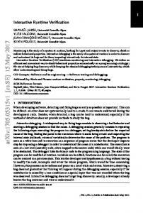
Figure 2: A BTT-FSM for the formula [](green -> !red U yellow) One should think of transitions using BTTs as naturally as possible; for example, if the BTTFSM in Figure 2 is in state 1 and a non-terminal event is received, then: first evaluate the predicate yellow; if true then stay in state 1 else evaluate green; if false then stay in state 1 else evaluate red; if true then report “formula violated” else move to state 2. When receiving a terminal event, 13
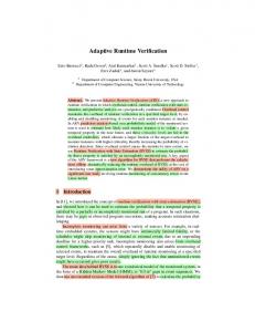
due to termination of monitoring, if the BTT-FSM is in state 1 then evaluate yellow and if true then return true else the opposite result of evaluating green. Only true/false messages are reported on terminal events, so the BTTs executed on terminal events are just Binary Decision Diagrams (BDDs) [5]. These FSMs can be either stored as data structures or generated as source code (case statements) which can further be compiled into actual monitors. Our FSMs can be exponential in the number of states (as function of the size of the initial LTL formula) but they only need to evaluate at most all the atomic state predicates in order to proceed to the next state when a new event is received, so the runtime overhead is actually linear with the number of distinct variables at worst. The size of our FSMs can become a problem when storage is a scarce resource, so we pay special attention to generating optimal FSMs. Interestingly, the number of state predicates to be evaluated tends to decrease with the number of states, so the overall monitoring overhead is also reduced. The drawback of generating an optimal BTT-FSM statically, i.e., before monitoring, is the exponential time/space required at startup (compilation). Therefore, we recommend this algorithm only in situations where the LTL formulae to monitor are relatively small in size and the runtime overhead is desired to be minimal. Informally, our algorithm to generate minimal FSMs from LTL formulae uses the rewriting based algorithm presented in the previous section statically on all possible events, until the set of formulae to which the initial LTL formula can “evolve” stabilizes. More precisely, it builds a FSM whose states are formulae and whose transitions are “events”, which are regarded as propositions on state boolean variables. Whenever a new potential state ψ, that is an LTL formula, is generated via a new event, that is a proposition on state variables p, from an existing state ϕ, ψ is semantically compared with all the previously generated states. If the ψ is not equivalent to any other existing state then it is added as a new state in the FSM. If found semantically equivalent to an already existing formula, say ψ 0 , then it is not added to the state space, but the current transition from ϕ to ψ 0 is updated by taking its disjunction with p (if no transition from ϕ to ψ 0 exists then a transition p is added). The semantical comparison is done using a validity checker for finite trace LTL that we have developed especially for this purpose. All these techniques are described and analyzed in more detail in [23]. Once the steps above terminate, the formulae ϕ, ψ, etc., encoding the states are not needed anymore, so we replace them by unique labels in order to reduce the amount of storage needed to encode the BTT-FSM. This algorithm can be relatively easily implemented in any programming language. We have, however, found Maude again a very elegant system, implementing this whole algorithm in about 200 lines of Maude code. This BTT-FSM generation algorithm, despite its overall startup exponential time, can be very useful when formulae are relatively short. For the traffic light controller requirement formula discussed previously, [](green -> (!red) U yellow), our algorithm generates in about 0.2 seconds the optimal BTT-FSM in Figure 3 (also shown in Figure 2 in flowchart notation). For simplicity, the State 1 2
Non-terminal event ? 1 : green ? red ? false : 2 : 1 yellow ? 1 : red ? false : 2
yellow
yellow
Terminal event ? true : green ? false : true yellow ? true : false
Figure 3: An optimal BTT-FSM for the formula [](green -> !red U yellow)
14
states true and false do not appear in Figure 3. Notice that the atomic predicate red does not need to be evaluated on terminal events and that green does not need to be evaluated in state 2. In this example, the colors are not supposed to exclude each other, that is, the traffic controller can potentially be both green and red. The LTL formulae on which our algorithm has the worst performance are those containing many nested temporal operators (which are not frequently used in specifications anyway, because of the high risk of getting them wrong). For example, it takes our algorithm 1.3 seconds to generate the minimal 3-state (true and false states are not counted) BTT-FSM for the formula a U (b U (c U d)) and 13.2 seconds to generate the 7-state minimal BTT-FSM for the formula ((a U b) U c) U d. It never took our current implementation more than a few seconds to generate the BTT-FSM of any LTL of interest for our applications (i.e., non-artificial). Figure 4 shows the generated BTT-FSM of some artificial LTL formulae, taking together less than 15 seconds to be generated. Formula ��a �(�a ∨ �¬a) �(a → �b) a U (b U c) a U (b U (c U d))
((a U b) U c) U d
State 1 1 1 2 1 2 1 2 3 1 2 3 4 5 6 7
next 1 1 a ? (b ? 1 : 2) : 1 b?1:2 c ? t : (a ? 1 : (b ? 2 : f)) c ? t : (b ? 2 : f) d?t:a?1:b?2:c?3:f d?t:b?2:c?3:f d?t:c?3:f d?t:c?1:b?4:a?5:f b?c?t:7:a?c?6:2:f b?d?t:c?1:4:a?d?6:c?3:5:f c?d?t:1:b?d?7:4:a?d?2:5:f b?d?c?t:7:c?1:4:a?d?c?6:2:c?3:5:f b?t:a?6:f c?t:b?7:a?2:f
end a?t:f t a ? (b ? t : f) : t b?t:f c?t:f c?t:f d?t:f d?t:f d?t:f d?t:f c?b?t:f:f d?b?t:f:f d?c?t:f:f d?c?b?t:f:f:f b?t:f c?t:f
Figure 4: Six BTT-FSMs generated in less than 15 seconds. The generated BTT-FSMs are monitored most efficiently on RAM machines, due to the fact that case statements are usually implemented via jumps in memory. Monitoring BTT-FSMs using rewriting does not seem appropriate because it would require linear time (as a function of the number of states) to extract the BTT associated to a state in a BTT-FSM. However, we believe that the algorithm presented in Subsection 4.1.3 is satisfactory in practice if one is willing to use a rewriting engine for monitoring. 4.2.2
Past Time LTL
We next focus on generating efficient monitors from formulae in past time LTL. The generated monitoring algorithm tests whether the formula is satisfied by a finite trace of events given as input and runs in linear time and space at worst. We only show how the generated monitoring algorithm looks for a concrete past time formula example, referring the interested reader to [24] for more details. We think that the next example is practically sufficient for the reader to foresee our general algorithm presented in detail in [24]. Let ↑ p → [q, ↓ (r ∨ s)) s be the past time LTL formula that 15
we want to generate code for. The formula states: “whenever p becomes true, then q has been true in the past, and since then we have not yet seen the end of r or s”. The code translation depends on an enumeration of the subformulae of the formula that satisfies the enumeration invariant: any formula has an enumeration number smaller than the numbers of all its subformulae. Let ϕ0 , ϕ1 , ..., ϕ8 be such an enumeration: ϕ0 ϕ1 ϕ2 ϕ3 ϕ4 ϕ5 ϕ6 ϕ7 ϕ8
= = = = = = = = =
↑ p → [q, ↓ (r ∨ s))s , ↑ p, p, [q, ↓ (r ∨ s))s , q, ↓ (r ∨ s), r ∨ s, r, s.
Note that the formulae have here been enumerated in a post-order fashion. One could have chosen a breadth-first order, or any other enumeration, as long as the enumeration invariant is true. The input to the generated program will be a finite trace t = e 1 e2 ...en of n events. The generated program will maintain a state via a function update : State ×Event → State, which updates the state with a given event. Our generated algorithms are dynamic programming algorithms speculating the recursive nature of the semantics of past time LTL as shown in Subsection 3.2. In order to illustrate the dynamic programming aspect of the solution, one can imagine recursively defining a matrix s[1..n, 0..8] of boolean values {0, 1}, with the meaning that s[i, j] = 1 iff t (i) |= ϕj . This would be the standard way of regarding the above satisfaction problem as a dynamic programming problem. An important observation is, however, that, like in many other dynamic programming algorithms, one doesn’t have to store all the table s[1..n, 0..8], which would be quite large in practice; in this case, one needs only s[i, 0..8] and s[i − 1, 0..8], which we’ll write now[0..8] and pre[0..8] from now on, respectively. It is now only a relatively simple exercise to write up the following algorithm for checking the above formula on a finite trace: State state ← {}; bit pre[0..8]; bit now[0..8]; Input: trace t = e1 e2 ...en ; /* Initialization of state and pre */ state ← update(state, e1 ); pre[8] ← s(state); pre[7] ← r(state); pre[6] ← pre[7] or pre[8]; pre[5] ← false; pre[4] ← q(state); pre[3] ← pre[4] and not pre[5]; pre[2] ← p(state); pre[1] ← false; pre[0] ← not pre[1] or pre[3]; /* Event interpretation loop */ for i = 2 to n do { state ← update(state, ei ); now[8] ← s(state); now[7] ← r(state); now[6] ← now[7] or now[8]; now[5] ← not now[6] and pre[6]; now[4] ← q(state); now[3] ← (pre[3] or now[4]) and not now[5]; now[2] ← p(state); now[1] ← now[2] and not pre[2]; now[0] ← not now[1] or now[3]; 16
if now[0] = 0 then output(‘‘property violated’’); pre ← now; }; In the following we explain the generated program. Declarations Initially a state is declared. This will be updated as the input event list is processed. Next, the two arrays pre and now are declared. The pre array will contain values of all subformulae in the previous state, while now will contain the value of all subformulae in the current state. The trace of events is then input. Such an event list can be read from a file generated from a program execution, or alternatively the events can be input on-the-fly one by one when generated, without storing them in a file first. Initialization The initialization phase consists of initializing the state variable and the pre array. The first event e1 of the event list is used to initialize the state variable. The pre array is initialized by evaluating all subformulae bottom up, starting with highest formula numbers, and assigning these values to the corresponding elements of the pre array; hence, for any i ∈ {0 . . . 8} pre[i] is assigned the initial value of formula ϕ i . The pre array is initialized in such a way as to maintain the view that the initial state is supposed stationary before monitoring is started. This in particular means that ↑ p is false, as well as is ↓ (r ∨ s), since there is no change in state (indices 1 and 5). The interval operator has the obvious initial interpretation: the first argument must be true and the second false for the formula to be true (index 3). Propositions are true if they hold in the initial state (indices 2, 4, 7 and 8), and boolean operators are interpreted the standard way (indices 0, 6). Event Loop The main evaluation loop goes through the event trace, starting from the second event. For each such event, the state is updated, followed by assignments to the now array in a bottom-up fashion similar to the initialization of the pre array: the array elements are assigned values from higher index values to lower index values, corresponding to the values of the corresponding subformulae. Propositional boolean operators are interpreted the standard way (indices 0 and 6). The formula ↑ p is true if p is true now and not true in the previous state (index 1). Similarly with the formula ↓ (r ∨ s) (index 5). The formula [q, ↓ (r ∨ s)) s is true if either the formula was true in the previous state, or q is true in the current state, and in addition ↓ (r ∨ s) is not true in the current state (index 3). At the end of the loop an error message is issued if now[0], the value of the whole formula, has the value 0 in the current state. Finally, the entire now array is copied into pre. Given a past time LTL formula, the analysis of this algorithm is straightforward. Its time complexity is Θ(n) where n is the length of the input trace, the constant being given by the size of the formula. The memory required is constant, since the length of the two arrays is the size of the formula. However, if one also includes the size of the formula, say m, into the analysis; then the time complexity is obviously Θ(n · m) while the memory required is 2 · (m + 1) bits. It is hard to find algorithms running faster than the above in practical situations, though some slight optimizations can be imagined as shown below. Even though a smart compiler can in principle generate good machine code from the code above, it is still worth exploring ways to synthesize directly optimized code especially because there are some attributes that are specific to the runtime observer which a compiler cannot take into 17
consideration. A first observation is that not all the bits in pre are needed, but only those which are used at the next iteration, namely 2, 3, and 6. Therefore, only a bit per temporal operator is needed, thereby reducing significantly the memory required by the generated algorithm. Then the body of the generated “for” loop becomes after (blind) substitution (we don’t consider the initialization code here): state ← update(state, ei ) now[3] ← r(state) or s(state) now[2] ← (pre[2] or q(state)) and not (not now[3] and pre[3]) now[1] ← p(state) if ((not (now[1] and not pre[1]) or now[2]) = 0) then output(‘‘property violated’’); which can be further optimized by boolean simplifications: state ← update(state, ej ) now[3] ← r(state) or s(state) now[2] ← (pre[2] or q(state)) and (now[3] or not pre[3]) now[1] ← p(state) if (now[1] and not pre[1] and not now[2]) then output(‘‘property violated’’); The most expensive part of the code above is clearly the function calls, namely p(state), q(state), r(state), and s(state). Depending upon the runtime requirements, the execution time of these functions may vary significantly. However, since one of the major concerns of monitoring is to affect the normal execution of the monitored program as little as possible, especially in online monitoring, one would of course want to evaluate the atomic predicates on states only if really needed, or rather to evaluate only those that, probabilistically, add a minimum cost. Since we don’t want to count on an optimizing compiler, we prefer to store the boolean formula as some kind of binary decision diagram. We have implemented a procedure in Maude, on top of a propositional calculus module, which generates all correct ( ? : )-expressions for ϕ, admittedly a potentially exponential number in the number of distinct atomic propositions in ϕ, and then chooses the shortest in size. Applied on the code above, it yields: state ← update(state, ej ) now[3] ← r(state) ? 1 : s(state) now[2] ← pre[3] ? pre[2] ? now[3] : q(state) : pre[2] ? 1 : q(state) now[1] ← p(state) if (pre[1] ? 0 : now[2] ? 0 : now [1 ]) then output(‘‘property violated’’); We would like to extend our procedure to take the evaluation costs of predicates into consideration. These costs can either be provided by the user of the system or be calculated automatically by a static analysis of predicates’ code, or even be estimated by executing the predicates on a sample of states. However, based on our examples so far, we conjecture that, given a boolean formula ϕ in which all the atomic propositions have the same cost, the probabilistically runtime optimal ( ? : )-expression implementing ϕ is exactly the one which is smallest in size. A further optimization would be to generate directly machine code instead of using a compiler. Then the arrays of bits now and pre can be stored in two registers, which would be all the memory 18
needed. Since all the operations executed are bit operations, the generated code is expected to be very fast. One could even imagine hardware implementations of past time monitors, using the same ideas, in order to enforce safety requirements on physical devices.
5
Concurrency Analysis
Logic based analysis of execution traces as described in the previous section can reveal domain specific high level errors, but it implies human intervention in designing the application requirements. However, many errors are lower level and are usually due to bad programming practice or lack of attention, and fortunately, an interesting portion of them can be revealed automatically. Even if some of these error patterns could be specified using adequate requirements formalisms and then enforced using the same logic-based approach as above, we think that this procedure is too heavy for this kind of errors, and that it is actually more appropriate to allow the users to attach designated efficient algorithms to JPaX. We have implemented the algorithms described below in both Maude and Java, but the current JPaX uses the Java implementations. Error pattern runtime analysis algorithms explore an execution trace and detect error potentials. The important and appealing aspect of these algorithms is that they find error potentials even in the case where errors do not explicitly occur in the examined execution trace. They are usually fast and scalable, and often catch the problems they are designed to catch, that is, the randomness in the choice of run does not seem to imply a similar randomness in the analysis results. The trade off is that they have less coverage than heavyweight formal methods (which may result in false negatives) and may suggest problems which, after a careful semantical analysis, turn out not to be errors (false positives). Two examples of such algorithms focusing on concurrency errors have been implemented in JPaX: a data race analysis algorithm and a deadlock analysis algorithm. The data race algorithm is essentially the Eraser algorithm [33], previously implemented in the Visual Threads tool [15] to work for C and C++ on Compaq hardware platforms, but in JPaX implemented to work for Java in a platform independent manner. The deadlock algorithm is an improvement of the deadlock algorithm presented in [15] that minimizes the number of false positives. This algorithm is in full described in [4]. The rest of this section shortly describes the data race and deadlock detection algorithms.
5.1
Data Race Analysis
We briefly describe here how data races can occur in concurrent Java programs, and how Eraser [33] has been implemented in JPaX to detect such. A data race occurs when two or more concurrent threads access a shared variable, at least one access is a write, and the threads use no explicit mechanism to prevent the accesses from being simultaneous. The Eraser algorithm detects data races by studying a single execution trace of the monitored program, trying to conclude whether there exist other traces where data races are possible. We illustrate the data race analysis with the Java program in Figure 5. The class Value contains an integer variable x, a synchronized method add that updates x by adding the content of another Value variable, and an unsynchronized method get that simply returns the value of x. Task is a thread class: its instances are started with the method start which executes the user defined method run. Two such tasks are started in Main, on two instances of the Value class, v1 and v2. When running JPaX with the Eraser option switched on, a data
19
1. 2. 3. 4. 5. 6. 7. 8. 9. 10. 11. 12. 13. 14. 15. 16. 17. 18. 19. 20. 21. 22. 23. 24. 25.
class Value{ private int x = 1; public synchronized void add(Value v){x = x + v.get();} public int get(){return x;} } class Task extends Thread{ Value v1; Value v2; public Task(Value v1,Value v2){ this.v1 = v1; this.v2 = v2; this.start(); } public void run(){v1.add(v2);} } class Main{ public static void main(String[] args){ Value v1 = new Value(); Value v2 = new Value(); new Task(v1,v2); new Task(v2,v1); } }
Figure 5: Example Program with data race race potential is found, reporting that the variable x in class Value is accessed unprotected by the two threads in lines 4 and 6, respectively. The generated warning message gives a scenario under which a data race might appear, summarizing the following. One Task thread can call the add method on the object v1 with the parameter Value object v2, whose content is thus read via the unsynchronized get method. The other thread can simultaneously do the same thing, i.e., call the add method on v2. Therefore, the content of v2 might be accessed simultaneously by the two threads. Note that Java allows two threads to operate simultaneously on an object if at least one of the threads does not synchronize on the object, which is the case here. Two data race warnings are actually emitted, since the the other task can perform the same behavior with v1 and v2 interchanged. Roughly, the algorithm is implemented in JPaX as follows. The instrumented byte code of the monitored program emits to the observer appropriate events when variables are written to or read from, and when locks are acquired or released as a result of entering/leaving Java’s synchronized statements or from calling/returning from synchronized methods. The observer maintains two data structures: a thread map that keeps track of all the locks owned at any point in time by each thread, and a variable map that associates with each (shared) variable the intersection of the set of locks that has been commonly owned by all accessing threads in the past. If this set ever becomes empty then a data race potential exists. More precisely, when a variable is accessed for the first time, the locks owned by the accessing thread at that moment are stored in the variable’s lock set. Subsequent accesses by other threads cause the set to be refined to its intersection with the locks owned by those threads. An extra state machine is also maintained for each variable to keep track of how many threads have accessed the variable and how (read/write). This is used to reduce the number of false positives, such as situations in which variables are initialized by a single thread without locks (which is safe) or several threads only read a variable after it has been initialized 20
(which is also safe). Deadlock Detection JPaX can detect resource deadlocks, where a collection of threads access a collection of resources in a cyclic manner. For example, a deadlock can occur if two threads T 1 and T2 need to synchronize on two objects A and B to do their respective task, but they synchronize on the objects in different order: T1 first synchronizes on A and then (without releasing A first) on B, while T 2 first synchronizes on B and then (without releasing B) on A. One can create such a situation in the previous Java example if one wrongly tries to repair the data race by also defining the get method in line 6 as synchronized: 6. public synchronized int get(){return x;}
It is clear now that the data race algorithm will indeed not return a warning anymore because the variable x can no longer be accessed simultaneously from two threads. However, there is a deadlock potential now and JPaX detects it. More precisely, when running JPaX on the modified program, a warning message is issued summarizing the fact that two object instances of the Value class are taken in a different order by the two Task threads. It also indicates the line numbers where the threads may potentially deadlock: line 4 where the get method called from add may block the second object. Note that any execution of the modified program will cause the deadlock warning to be issued, hence there are guaranteed no false negatives for this example. This pleasing property can, however, not be expected for realistic programs. Conversely, deadlock potentials might be reported in general even if those deadlocks will never appear in any execution of the program (false positives). For this program, however, there are neither any false positives. The runtime deadlock analysis algorithm needs only a subset of the events generated for the data race algorithm, namely those related to lock acquisitions and releases that result from entering/leaving Java’s synchronized statements or from calling/returning from synchronized methods. Start and join events are also needed and are used to reduce false positives. Two data structures are maintained in the observer: as in the data race algorithm a thread map keeps track of the locks owned by each thread, while a second data structure, a lock graph, updates a graph that accumulates as nodes all the locks taken by any thread during an execution. An edge is introduced from a lock L1 to a lock L2 whenever a thread that already holds L 1 acquires L2 . If during the execution of the program this graph becomes cyclic, a deadlock potential is reported. This simple algorithm can reveal complex deadlock potentials between any number of threads. The just presented algorithm is the one also described in [15]. The algorithm in JPaX is, however, further augmented to yield less false positives, as described in detail in [4]. Three categories of false positives are eliminated by the extended algorithm. The first category, single threaded cycles, refers to cycles that are created by one single thread. Guarded cycles refer to cycles that are guarded by a gate lock ”taken higher up” by all involved threads. Finally, thread segmented cycles refer to cycles between thread segments that cannot possibly execute concurrently. To illustrate a guarded cycle consider the program in Figure 5, and assume that line number 6 has been modified to include the synchronized keyword, such that a deadlock situation is possible. If we now further modify the program as follows, by adding a synchronization on a single gate lock before other locks are taken, then no deadlock can occur: class Task extends Thread{
21
static Object gate = new Object(); ... public void run(){ synchronized(gate){ v1.add(v2); } }
6
Conclusions
We have presented work done in the context of the the JPaX runtime verification tool. JPaX provides an integrated environment for monitoring the execution of Java programs. A program is instrumented to generate an execution trace when run, which can then be examined by various specialized algorithms that we have described. Amongst these are algorithms for testing the trace against future time and past time temporal logic formulae. We have presented how such logics can be formulated in a rewriting logic, and how the Maude rewriting system can be used to monitor the validity of the execution trace against such formulae. It has also been shown how observer automata can be generated from future time and past time temporal logic formulae, to achieve even more efficient observer algorithms. An interesting observation is, however, that the implementation of these logics in the Maude rewriting system resulted in very small code, and still compared very well with the automata solutions in efficiency. Using Maude for defining new observer logics seems to be an excellent prototyping approach at least, and even seems fast enough for practical monitoring. We furthermore presented algorithms for performing data race and deadlock analysis. These algorithms in their basic form have been implemented in other systems, but the data race algorithm has here been adapted to work for Java, and the deadlock algorithm has been extended to yield fewer false positives. Future work includes studying more powerful logics, including real-time information and data. Concerning concurrency analysis, we are currently expanding the kinds of errors that can be found by simple trace analysis. We expect to combine the runtime monitoring environment with a test case generation environment that can generate many execution traces. Such a test case environment can include a stateless model checker. Runtime verification can be used during testing or after deployment, during operation of the software. An important and non-trivial research topic is how to correct the behavior of a program on-the-fly when properties are violated.
References [1] 1st CAV Workshop on Runtime Verification (RV’01). In K. Havelund and G. Ro¸su, editors, Proceedings of Runtime Verification (RV’01), volume 55(2) of Electronic Notes in Theoretical Computer Science. Elsevier Science, 2001. [2] 2nd CAV Workshop on Runtime Verification (RV’02). In K. Havelund and G. Ro¸su, editors, Proceedings of Runtime Verification (RV’02), volume 70(4) of Electronic Notes in Theoretical Computer Science. Elsevier Science, 2002. [3] T. Ball, A. Podelski, and S. Rajamani. Boolean and Cartesian Abstractions for Model Checking C Programs. In Proceedings of TACAS’01: Tools and Algorithms for the Construction and Analysis of Systems, LNCS, Genova, Italy, April 2001.
22
[4] S. Bensalem and K. Havelund. Reducing False Positives in Runtime Analysis of Deadlocks. Submitted for publication, October 2002. [5] R. E. Bryant. Graph-based algorithms for Boolean function manipulation. IEEE Transactions on Computers, C-35(8):677–691, August 1986. [6] M. Clavel, F. J. Dur´an, S. Eker, P. Lincoln, N. Mart´ı-Oliet, J. Meseguer, and J. F. Quesada. Maude: Specification and Programming in Rewriting Logic, March 1999. Maude System documentation at http://maude.csl.sri.com/papers. [7] M. Clavel, F. J. Dur´an, S. Eker, P. Lincoln, N. Mart´ı-Oliet, J. Meseguer, and J. F. Quesada. The Maude system. In Proceedings of the 10th International Conference on Rewriting Techniques and Applications (RTA-99), volume 1631 of LNCS, pages 240–243, Trento, Italy, July 1999. Springer-Verlag. System description. [8] M. Clavel, F. J. Dur´an, S. Eker, P. Lincoln, N. Mart´ı-Oliet, J. Meseguer, and J. F. Quesada. A Maude Tutorial, March 2000. Manuscript at http://maude.csl.sri.com/papers. [9] S. Cohen. Jtrek. Compaq, http://www.compaq.com/java/download/jtrek. [10] J. Corbett, M. B. Dwyer, J. Hatcliff, C. S. Pasareanu, Robby, S. Laubach, and H. Zheng. Bandera : Extracting Finite-state Models from Java Source Code. In Proceedings of the 22nd International Conference on Software Engineering, Limerich, Ireland, June 2000. ACM Press. [11] D. Drusinsky. The Temporal Rover and the ATG Rover. In SPIN Model Checking and Software Verification, volume 1885 of LNCS, pages 323–330. Springer, 2000. [12] B. Finkbeiner, S. Sankaranarayanan, and H. Sipma. Collecting Statistics over Runtime Executions. In K. Havelund and G. Ro¸su, editors, Proceedings of Runtime Verification (RV’02), Electronic Notes in Theoretical Computer Science. Elsevier Science, to appear, 2002. [13] D. Giannakopoulou and K. Havelund. Automata-Based Verification of Temporal Properties on Running Programs. In Proceedings, International Conference on Automated Software Engineering (ASE’01), pages 412–416. Institute of Electrical and Electronics Engineers, 2001. Coronado Island, California. [14] P. Godefroid. Model Checking for Programming Languages using VeriSoft. In Proceedings of the 24th ACM Symposium on Principles of Programming Languages, pages 174–186, Paris, France, January 1997. [15] J. Harrow. Runtime Checking of Multithreaded Applications with Visual Threads. In SPIN Model Checking and Software Verification, volume 1885 of LNCS, pages 331–342. Springer, 2000. [16] K. Havelund. Using Runtime Analysis to Guide Model Checking of Java Programs. In SPIN Model Checking and Software Verification, volume 1885 of LNCS, pages 245–264. Springer, 2000.
23
[17] K. Havelund, S. Johnson, and G. Ro¸su. Specification and Error Pattern Based Program Monitoring. In Proceedings of the European Space Agency workshop on On-Board Autonomy, Noordwijk, The Netherlands, October 2001. [18] K. Havelund and T. Pressburger. Model Checking Java Programs using Java PathFinder. International Journal on Software Tools for Technology Transfer, 2(4):366–381, April 2000. Special issue of STTT containing selected submissions to the 4th SPIN workshop, Paris, France, 1998. [19] K. Havelund and G. Ro¸su. Testing Linear Temporal Logic Formulae on Finite Execution Traces. RIACS Technical report, http://ase.arc.nasa.gov/pax, November 2000. [20] K. Havelund and G. Ro¸su. Java PathExplorer – A Runtime Verification Tool. In Proceedings of the 6th International Symposium on Artificial Intelligence, Robotics and Automation in Space (i-SAIRAS’01), Montreal, Canada, June 2001. [21] K. Havelund and G. Ro¸su. Monitoring Java Programs with Java PathExplorer. In K. Havelund and G. Ro¸su, editors, Proceedings of Runtime Verification (RV’01), volume 55 of Electronic Notes in Theoretical Computer Science. Elsevier Science, 2001. [22] K. Havelund and G. Ro¸su. Monitoring Programs using Rewriting. In Proceedings, International Conference on Automated Software Engineering (ASE’01), pages 135–143. Institute of Electrical and Electronics Engineers, 2001. Coronado Island, California. [23] K. Havelund and G. Ro¸su. A Rewriting-based Approach to Trace Analysis. Submitted for journal publication, September 2002. [24] K. Havelund and G. Ro¸su. Synthesizing monitors for safety properties. In Tools and Algorithms for Construction and Analysis of Systems (TACAS’02), volume 2280 of Lecture Notes in Computer Science, pages 342–356. Springer, 2002. EASST best paper award at ETAPS’02. [25] G. J. Holzmann and M. H. Smith. A Practical Method for Verifying Event-Driven Software. In Proceedings of ICSE’99, International Conference on Software Engineering, Los Angeles, California, USA, May 1999. IEEE/ACM. [26] J. Hsiang. Refutational Theorem Proving using Term Rewriting Systems. PhD thesis, University of Illinois at Champaign-Urbana, 1981. [27] I. Lee, S. Kannan, M. Kim, O. Sokolsky, and M. Viswanathan. Runtime Assurance Based on Formal Specifications. In Proceedings of the International Conference on Parallel and Distributed Processing Techniques and Applications, 1999. [28] Z. Manna and A. Pnueli. The Temporal Logic of Reactive and Concurrent Systems. Springer, New York, 1992. [29] Z. Manna and A. Pnueli. Temporal Verification of Reactive Systems: Safety. Springer, New York, 1995. [30] J. Meseguer. Conditional rewriting logic as a unified model of concurrency. Theoretical Computer Science, pages 73–155, 1992. 24
[31] J. Meseguer. Membership algebra as a logical framework for equational specification. In Proceedings, WADT’97, volume 1376 of LNCS, pages 18–61. Springer, 1998. [32] G. Ro¸su and K. Havelund. Synthesizing Dynamic Programming Algorithms from Linear Temporal Logic Formulae. RIACS Technical report, http://ase.arc.nasa.gov/pax, January 2001. [33] S. Savage, M. Burrows, G. Nelson, P. Sobalvarro, and T. Anderson. Eraser: A Dynamic Data Race Detector for Multithreaded Programs. ACM Transactions on Computer Systems, 15(4):391–411, November 1997. [34] S. D. Stoller. Model-Checking Multi-threaded Distributed Java Programs. In SPIN Model Checking and Software Verification, volume 1885 of LNCS, pages 224–244. Springer, 2000. [35] W. Visser, K. Havelund, G. Brat, and S. Park. Model Checking Programs. In Proceedings of ASE’2000: The 15th IEEE International Conference on Automated Software Engineering. IEEE CS Press, September 2000.
25