An overview of topic modeling and its current ... - Semantic Scholar
Recommend Documents
It has been shown that nicotine crosses biological membranes and the blood brain barrier ... Keywords: Nicotine; Metabolism of nicotine; Effects of nicotine.
investigated (Dave et al., 1995). It was shown that .... Abood, L.G., Grassi, S., Noggle, H.D., 1985. ..... Rakowicz, E.M., David, S., McIntosh, G., Smith, M., 1994.
Transaction Level Modeling: An Overview. Lukai Cai ... Center for Embedded Computer Systems ... place by calling interface functions of these channel models.
Apr 14, 2014 - In these Protestant families parents raise their children in a religious way by ...... âA History of Research on Parenting Strategies and Children's ...
primarily consists of a number of event handler blocks, representing its di erent execution-time states. The body of a manifold may also contain additional ...
field, what relations and influences exist between top- ics within and across fields, as well as what trends can be established for some of the world's natural lan-.
development of multi-agent systems (MAS). For this ... of trends in modelling this kind of systems (section 3). .... development of telecom applications using agent.
According to Mason (2002), about ... 1999; Williams, 2001). ..... is designed as an integrated component of a Web-based Learning Management System (Mason.
Nov 17, 2013 - ... state-of-the-art parallel LDA algorithms on the multi-processor architecture. ... because big data have become increasingly common in recent ...
Keywords: cointegration, conditional models, data mining, diagnostic testing, dy- ...... the choice of econometric techn
topic lttm model of Wikipedia representing Maryland, Southeast. Asia, The .... computer company has been given the title âApple Inc.â. Another option is to add.
Osama Khalifa, David Corne, Mike Chantler, Fraser Halley. Heriot-Watt ...... [24] MALLET: A Machine Learning for Language Toolkit, http://mallet.cs.umass.edu.
Flegal KM, Carroll MD, Kuczmarski RJ, Johnson CL. Over weight and obesity in the ... Jacob CS, Katherine MH. Assessing obesity classification and ...
Apr 14, 2004 - The discovery of 'ob' gene, which was mapped to chromosome .... of obesity requires the development of coherent strategies that tackle the .... Orlistat is a potent and irreversible inhibitor of gastric, ... Lipase inhibitor, ATL-962.
discovery of 'ob' gene, which was mapped to chromosome 7, has led to a ... These factors play a critical role in the development of obesity by unmasking genetic or .... Orlistat is a potent and irreversible inhibitor of gastric, pancreatic lipases.
Jul 31, 2009 - PAT: This is an analytical performance analysis tool from Bell Labs and could be ... QNA: This is a queuing network analyzer analytical tool.
Jul 31, 2009 - library development potential is enormous. 13.COMNET 111: This is a trace driven tool sold by CACI. This tool replaces LNETII and COMNET ...
An emphasis on treating service users as 'customers' and on the application of generic quality improvement ..... OECD, PUMA/SMO(99)4/FINAL. 11. POLLITT, C.
(TDS) can be considered a part of the more general study temporal text mining (TTM) that â... .... framework to model topics with a network structure, by regularizing the ..... âSupervised Topic Models,â Advances in Neural Information Processin
Jun 28, 2016 - mass of the chili peppers and, together with salt, represent the most consumed .... obtained by the capsaicin-evoked response of C-fibers in the cat saphenous nerve. ...... of capsaicin in carcinogen-induced skin cancer in mice [226].
2 Spearman's factor analysis as a primary source of structural equation modeling ...... Tucker, L.R.: Some mathematical notes on three-mode factor analysis.
Mar 31, 2007 - This PDF is available for free download from a site hosted by Medknow Publications. (www.medknow.com). Indian Journal of Medical ...
Wen et al. (2006),. Zhang et al. (2006b) and Sun et al. (2006). 1158030E 102 m. Typical red earth. Pinus elliottii, Pinus massoniana, Cunninghamia lanceolata ...
toxicogenomics. BMC Syst Biol 8(1):1â11. Li W, McCallum A (2006) Pachinko allocation: DAG-structured mixture models of topic correlations. In: Proceedings of ...
Liu et al. SpringerPlus (2016) 5:1608 DOI 10.1186/s40064-016-3252-8
Open Access
REVIEW
An overview of topic modeling and its current applications in bioinformatics Lin Liu1,2, Lin Tang3, Wen Dong1, Shaowen Yao4* and Wei Zhou4* *Correspondence: [email protected]; zwei@ ynu.edu.cn 4 National Pilot School of Software, Yunnan University, Kunming 650091, Yunnan, China Full list of author information is available at the end of the article
Abstract Background: With the rapid accumulation of biological datasets, machine learning methods designed to automate data analysis are urgently needed. In recent years, socalled topic models that originated from the field of natural language processing have been receiving much attention in bioinformatics because of their interpretability. Our aim was to review the application and development of topic models for bioinformatics. Description: This paper starts with the description of a topic model, with a focus on the understanding of topic modeling. A general outline is provided on how to build an application in a topic model and how to develop a topic model. Meanwhile, the literature on application of topic models to biological data was searched and analyzed in depth. According to the types of models and the analogy between the concept of document-topic-word and a biological object (as well as the tasks of a topic model), we categorized the related studies and provided an outlook on the use of topic models for the development of bioinformatics applications. Conclusion: Topic modeling is a useful method (in contrast to the traditional means of data reduction in bioinformatics) and enhances researchers’ ability to interpret biological information. Nevertheless, due to the lack of topic models optimized for specific biological data, the studies on topic modeling in biological data still have a long and challenging road ahead. We believe that topic models are a promising method for various applications in bioinformatics research. Keywords: Topic model, Bioinformatics, Probabilistic generative model, Clustering, Classification
is a genuine topic model. Published after PLSA, latent Dirichlet allocation (LDA) proposed by Blei et al. (2003) is an even more complete probabilistic generative model and is the extension of PLSA. Nowadays, there is a growing number of probabilistic models that are based on LDA via combination with particular tasks. Nonetheless, all the abovementioned topic models have initially been introduced in the text analysis community for unsupervised topic discovery in a corpus of documents. Since the emergence of topic models, researchers have introduced this approach into the fields of biological and medical document mining. Because of its superiority in analysis of large-scale document collections, better results have been obtained in such fields as biological/biomedical text mining (Andrzejewski 2006; Wang et al. 2009, 2013, 2016; Bisgin et al. 2011, 2012; Chen et al. 2012c; Song and Kim 2013) and clinical informatics (Arnold et al. 2010; Sarioglu et al. 2012; Zeng et al. 2012; Zhang et al. 2012b; Howes et al. 2013; Sarioglu et al. 2013; Hu et al. 2014; Huang et al. 2014). On the other hand, most of these studies follow the classic text-mining method of a topic model. In recent years, we have been witnessing exponential growth of biological data, such as microarray datasets. This situation also poses a great challenge, namely, how to extract hidden knowledge and relations from these data. As mentioned above, topic models have emerged as an effective method for discovering useful structure in collections. Therefore, a growing number of researchers are beginning to integrate topic models into various biological data, not only document collections. In these studies, we find that topic models act as more than a classification or clustering approach. They can model a biological object in terms of hidden “topics” that can reflect the underlying biological meaning more comprehensively. Therefore, topic models were recently shown to be a powerful tool for bioinformatics. In this paper, the existing studies on topic modeling in biological data are analyzed from different points of view, and then the problems and prospects are discussed. To the best of our knowledge, this is the first effort to review the application and development of topic models for bioinformatics. In contrast, the studies related to topic models applied to pure biological or medical text mining are outside the scope of this paper. The rest of this paper is structured as follows. In “Topic modeling” section, the general outline of how to build an application in accordance with a topic model is given. In particular, LDA and PLSA are presented by means of the terminology and notation of the document analysis context. “The development of a topic model” and “The toolkits for topic models” sections summarize a large number of topic models that evolved from LDA and the existing topic model toolkits. In “The use of topic models in bioinformatics” sections, numerous relevant papers on topic models—as applied to bioinformatics—are discussed in keeping with three themes: the tasks of a topic model, the types of models, and an analogy between the concept “document-topic-word” and a biological object. In “The trends in applications of topic models to bioinformatics” sections, we give our thoughts on some of the promising unexplored directions for the use of topic modeling in biological applications. Finally, the conclusions are drawn.
Page 2 of 22
Liu et al. SpringerPlus (2016) 5:1608
Page 3 of 22
Topic modeling To better understand how to use a topic model in bioinformatics, we first describe the basic ideas behind topic modeling by means of a diagram. Figure 1 (The diagram of topic modeling) illustrates the key steps of topic modeling, including the bag of words (BoW), model training, and model output. We first assume that there are N documents, V words, and K topics in a corpus. Then, we discuss each component of this diagram in detail. The BoW
In natural language processing, a document is usually represented by a BoW that is actually a word-document matrix. An example of a BoW is shown in Table 1. As shown in Table 1, there are four words (gene, protein, pathway, and microarray) and six documents (d1–d6) in this corpus. Value wij in the matrix represents the frequency of word i in document j. For example, w3,1 = 1 means that the frequency of the word “pathway” in document d1 is 1.0. It is obvious that the number of words is fixed in a corpus, and the collection of these words constitutes a vocabulary. In short, the corpus is represented by the BoW it contains. A BoW is a simplified representation of a corpus as the input of topic modeling. Likewise, if we want to process biological data rather than a corpus, we also need to represent biological data as a BoW: to specify which is the document and which is the word in the field of biology. For instance, in the problem of genomic sequence classification, La Rosa et al. (2015) consider genomic sequences to be documents and small fragments of a DNA string of size k to be words. Then, the BoW of genomic sequences can be calculated easily. After construction of the BoW, it serves as the input of the next step in topic modeling. Suppose there are N documents and V words in a corpus; thus, the BoW of this corpus is an N × V matrix. From the description of the BoW above, we can deduce that the order of words in a document does not affect the representation of the BoW. Put another way, the words in
K
corpus document
N
BoW
V
2 0 1
5 7 0
0 0 2
N 1 defining the generation process or graph model
0.239
0.028
0.132
0.056
0.591
0.325
0.012
0.231
0.051
0.018
0.132
0.56
0.191
0.025
0.012
0.131
V
input
2 estimation of parameters
output
model training K
Fig. 1 The diagram of topic modeling
Table 1 An example of a BoW d1
d2
d3
d4
d5
d6
Gene
2
0
3
0
0
0
Protein
0
5
0
0
0
0
Pathway
1
2
0
0
0
0
Microarray
0
0
3
6
0
0
Liu et al. SpringerPlus (2016) 5:1608
Page 4 of 22
the document are exchangeable. Moreover, the documents in a corpus are independent: there is no relation among the documents. The exchangeability of words and documents could be called the basic assumptions of a topic model. These assumptions are available in both PLSA and LDA. Nevertheless, in several variants of topic models, a basic assumption was relaxed. The summary of variants of LDA is provided in section “The development of a topic model”. Model training
In a BoW, the dimensionality of word space may be enormous, and the BoW reflects only the words of the original texts. In contrast, the most important thing people expect to know about a document is the themes rather than words. The aim of topic modeling is to discover the themes that run through a corpus by analyzing the words of the original texts. We call these themes “topics.” The classic topic models are unsupervised algorithms (that do not require any prior annotations or labeling of the documents), and the “topics” were discovered during model training. The definition of a topic
In topic modeling, a “topic” is viewed as a probability distribution over a fixed vocabulary. As an example, Table 2 (The top five most frequent words from three topics) illustrates three “topics” that were discovered in a corpus, including “Protein,” “Cancer,” and “Computation” (Blei 2012). As shown in Table 2, the probabilities of each word in a “topic” were sorted in the descending order. The top five most frequent words reflect the related concepts of each “topic”: “Topic 1” is about a protein, “Topic 2” is about cancer, and “Topic 3” is about computation. In short, each “topic” is a mixture of “words” in a vocabulary. Similarly, in topic modeling, each document is a mixture of “topics.” As shown in Fig. 2 (The topic distribution of a document), we assumed that K is the number of topics. Above all, the key idea behind topic modeling is that documents show multiple topics, and therefore the key question of topic modeling is how to discover a topic distribution over each document and a word distribution over each topic, which represent an N × K matrix and a K × V matrix, respectively. The output of a topic model is then obtained in the next two steps. The generative process
First, topic modeling needs to simulate the generative process of documents. Each document is assumed to be generated as follows: for each word in this document, choose a
Table 2 The top five most frequent words from three topics Topics
Protein
Cancer
Computation
Words
Protein
Tumor
Computer
Cell
Cancer
Model
Gene
Diseases
Algorithm
DNA
Death
Data
Polypeptide
Medical
Mathematical
Liu et al. SpringerPlus (2016) 5:1608
Fig. 2 The topic distribution of a document
topic assignment and choose the word from the corresponding topic. PLSA and LDA are relatively simple topic models; in particular, other topic modes that appeared in recent years are more or less related to LDA. Therefore, understanding LDA is important for the extended application of topic models. We use PLSA and LDA as examples to describe the generative process in this paper. In PLSA, suppose d denotes the label of a document, z is a topic, w represents a word, and Nd is the number of words in document d. Therefore, P(z|d) denotes the probability of topic z in document d, and P(w|z) means the probability of word w in topic z. Then, for PLSA, the generative procedure for each word in the document is as follows: (a) Randomly choose a topic from the distribution over topics (P(z|d)); (b) randomly choose a word from the corresponding distribution over the vocabulary (P(w|z)). The pseudocode is as follows:
Besides the descriptive approach of the generative process above, a graphical model can also reflect the generative process of documents. As shown in Fig. 3 (The graphical model of PLSA), the box indicates repeated contents; the number in the lower right corner is the number of repetitions. The gray nodes represent observations; white nodes represent hidden random variables or parameters. The arrows denote dependences.
Fig. 3 The graphical model of PLSA
Page 5 of 22
Liu et al. SpringerPlus (2016) 5:1608
In LDA, the two probability distributions, p(z|d) and p(w|z), are assumed to be multinomial distributions. Thus, the topic distributions in all documents share the common Dirichlet prior α, and the word distributions of topics share the common Dirichlet prior η. Given the parameters α and η for document d, parameter θd of a multinomial distribution over K topics is constructed from Dirichlet distribution Dir(θd|α). Similarly, for topic k, parameter βk of a multinomial distribution over V words is derived from Dirichlet distribution Dir(βk|η). As a conjugate prior for the multinomial, the Dirichlet distribution is a convenient choice as a prior and can simplify the statistical inference in LDA. Therefore, in PLSA, by contrast, any common prior probability distribution was not specified for p(z|d) andp(w|z). Naturally, there are no α and η in the generative process of PLSA.
Then, we can summarize LDA as a generative procedure: Likewise, we can use a graphical model to represent LDA, as shown in Fig. 4 (The graphical model of LDA). The parameter estimation
As described above, the goal of topic modeling is to automatically discover the topics in a collection of documents. The documents themselves are examined, whereas the topic structure—the topics, per-document topic distributions, and the per-document per-word topic assignments—is hidden structure. The central computational problem
Fig. 4 The graphical model of LDA
Page 6 of 22
Liu et al. SpringerPlus (2016) 5:1608
Page 7 of 22
for topic modeling is how to use the documents under study to infer the hidden topic structure. This task can be thought of as a “reversal” of the generative process; the task of parameter estimation can be summarized as follows: given the corpus, estimate the posterior distribution of unknown model parameters and hidden variables. According to the generative procedure of PLSA, the log-likelihood of a corpus is given by L= n(d, w) log p(d, w) d∈N w∈V
where n(d, w) denotes the number of times word w appeared in document d, and log p(d, w) means the probability of (d, w). Then, the maximum likelihood estimator is used to obtain the model parameters (p(z|d), p(w|z)), such as the expectation maximization algorithm (EM) (Moon 1996). For an LDA model, given the parameters α and η, the empirical values are α = 50/K and η = 0.01. The joint distribution of topic mixture θ, word mixture β, a set of K topics z, and a set of N words w that constitute the document is expressed as
p(β, θ, w, z|α, η) =
N d=1
p(θd |α)
Nd n=1
p(zdn |θd )p(wdn |zdn , β)
K p βk |η k=1
Via the joint distribution, we can estimate p(β, θ, z|w), the posterior distribution of unknown model parameters and hidden variables: the central task of learning in a topic model. Classic approaches to an inference algorithm in LDA are expectationpropagation (EP) (Minka and Lafferty 2002), collapsed Gibbs sampling (Griffiths and Steyvers 2004), and variational Bayesian inference (VB) (Blei et al. 2003). Besides, Teh et al. (2006b) proposed a collapsed variational Bayesian, which combines collapsed Gibbs sampling and VB. Every kind of algorithm has its own advantages: the variational approach is arguably faster computationally, but the Gibbs sampling approach is in principle more accurate (Porteous et al. 2008). We need to choose them according to efficiency, complexity, accuracy, and the generative process. Regardless of the method that we choose, their aim is the same: given the objective functions for optimization, to obtain an estimate of a parameter. For model training, the inference algorithm of parameters is based on the generative process or a graph model and is the most complex and important stage in topic modeling. For brevity, however, these methods will not be described in detail. Moreover, if we use only LDA, PLSA, or other existing topic models directly, their inference algorithm of parameters is ready-made, and the tasks that we need to do are construction of data input and parameter initialization. Model outputs
For PLSA and LDA, the outputs of the model include two matrices: one is the topic probability distributions over documents, represented by an N × K matrix; the other is the word probability distributions over topics, represented by a K × V matrix. “Topics” can be identified by estimating the parameters in the case of known documents. If the number of “topics” was specified as K, then K “topics” could be obtained through model
Liu et al. SpringerPlus (2016) 5:1608
training. After that, the word term space of documents is transformed into “topic” space. It is obvious that “topic” space is smaller than word space (K