Transaction Level Modeling: An Overview. Lukai Cai ... Center for Embedded Computer Systems ... place by calling interface functions of these channel models.
Transaction Level Modeling: An Overview Lukai Cai and Daniel Gajski Center for Embedded Computer Systems University of California, Irvine Irvine, CA 92697, USA {lcai,gajski}@cecs.uci.edu
ABSTRACT Recently, the transaction-level modeling has been widely referred to in system-level design community. However, the transaction-level models(TLMs) are not well defined and the usage of TLMs in the existing design domains, namely modeling, validation, refinement, exploration, and synthesis, is not well coordinated. This paper introduces a TLM taxonomy and compares the benefits of TLMs’ use.
;; ;;; ;;
Communication
Cycletimed
D
Approximatetimed
C
Categories and Subject Descriptors C.0 [Computer Systems Organization]: General
Untimed
A Untimed
General Terms Design
F
E
A. Specification model B. Component-assembly model C. Bus-arbitration model D. Bus-functional model E. Cycle-accurate computation model F. Implementation model
B
Approximatetimed
Cycletimed
Computation
Figure 1: System modeling graph
Keywords Transaction level model, modeling, validation, refinement, exploration, synthesis
1. INTRODUCTION In order to handle the ever increasing complexity of systemon-chips (SoCs) and time-to-market pressures, the design abstraction has been raised to the system level in order to increase design productivity. This higher level of abstraction generated large interest in transaction-level modeling, synthesis, and verification [10][12]. In a transaction-level model (TLM), the details of communication among computation components are separated from the details of computation components. Communication is modeled by channels, while transaction requests take place by calling interface functions of these channel models. Unnecessary details of communication and computation are hidden in a TLM and may be added later. TLMs speed up simulation and allow exploring and validating design alternatives at the higher level of abstraction. However, the definition of TLMs is not well understood. Without clear definition of TLMs, not only the predefined
Permission to make digital or hard copies of all or part of this work for personal or classroom use is granted without fee provided that copies are not made or distributed for profit or commercial advantage and that copies bear this notice and the full citation on the first page. To copy otherwise, to republish, to post on servers or to redistribute to lists, requires prior specific permission and/or a fee. CODES+ISSS’03, October 1–3, 2003, Newport Beach, California, USA. Copyright 2003 ACM 1-58113-742-7/03/0010 ...$5.00.
TLMs cannot be easily reused, but also the usage of TLMs in the existing design domains, namely modeling, validation, refinement, exploration, and synthesis, cannot be systematically developed. Consequently, the inherent advantages of TLMs don’t effectively benefit designers. In order to eliminate some ambiguity of TLMs, this paper attempts to explicitly define several transaction-level models, each of which is adopted for different design purpose. It also explores the usage of defined TLMs under a general design flow and analyzes how the TLMs are used in the design domains. This paper is organized as follows: Section 2 reviews the related work; Section 3 defines four TLMs; Section 4 introduces the usage of TLMs in different design domains; Finally, the conclusion is given in section 5.
2.
RELATED WORK
The concept of TLM first appears in system level language and modeling domain. [10] defines the concept of a channel, which enables separating communication from computation. It proposes four well-defined models at different abstraction levels in a top-down design flow. Some of these models can be classified as TLMs. However, the capabilities of TLMs are not explicitly emphasized. [12] broadly describes the TLM features based on the channel concept and presents some design examples. However, the TLMs are not well defined and the usage of TLMs in the existing design domains is not addressed. [10] [12] also demonstrate that both SpecC [3] and SystemC [2] support transaction level modeling using the channel concept. The TLMs can be used in top-down approaches such as
proposed by SCE [6] that starts design from the system behavior representing the design’s functionality, generates a system architecture from the behavior, and gradually reaches the implementation model by adding implementation details. In comparison to the top-down approaches, meetin-the-middle approaches [13] map the system behavior to the predefined system architecture, rather than generating the architecture from the behavior. An example of meetin-the-middle approach is VCC [5] for architecture estimation/exploration and N2C [1] for interface synthesis. Unlike above two approaches, bottom-up approaches assemble the existing computation components by inserting wrappers among them. Bottom-up approaches, such as proposed in [9], focus on component reuse and wrapper generation. All of above three design practices fully or partly cover the design from the system behavior to the detailed system implementation, which exhibits great potential of employing TLMs. Some other research groups have applied TLMs in the design. [14] adopts TLMs to ease the development of embedded software. [15] defines a TLM with certain protocol details in a platform-based design, and uses it to integrate components at the transaction level. [11] implements co-simulation across-abstraction level using channels, which implies the usage of TLM. Each of above research addresses only one limited aspect of TLMs.
B1 v1 = a*a;
v1
B2B3 B3
B2 v2 = v1 + b*b;
v3= v1- b*b;
v2
v3
B4
v4 = v2 + v3; c = sequ(v4);
Figure 2: The example of specification model PE1 B1
cv11
v1 = a*a;
PE3
3. TRANSACTION LEVEL MODELS
B3
cv12
In order to simplify the design process, designers generally use a number of intermediate models. The intermediate models slice the entire design into several smaller design stages, each of which has a specific design objective. Since the models can be simulated and estimated, the result of each of these design stages can be independently validated. In order to relate different models, we introduce the system modeling graph (shown in Figure 1) [8]. X-axis in the graph represents computation and y-axis represents communication. On each axis, we have three degrees of time accuracy: un-timed, approximate-timed, and cycle-timed. Un-timed computation/communication represents the pure functionality of the design without any implementation details. Approximate-timed computation/communication contains system-level implementation details, such as the selected system architecture, the mapping relations between processes of the system specification and the processing elements of the system architecture. The execution time for approximate-timed computation/communication is usually estimated at the system level without cycle-accurate RTL (register transfer level) /ISS (instruction set simulation) level evaluation [5]. Cycle-timed computation/communication contains implementation details at both system level and the RTL/ISS level, such that cycle-accurate estimation can be obtained. Inspired by [10] [12], we define six abstraction models in the system modeling graph, which are indicated by circles. Among them, component-assembly model, bus-arbitration model, bus-functional model, and cycle-accurate computation model are TLMs, which are indicated by shaded circles. Specification model. It describes the system functionality and is free of any implementation details. This model is similar to the specification model in [10] and untimed functional model in [12]. It can model the data transfer between processes through variable accessing without using
v3= v1- b*b;
v3
PE2 B2 v2 = v1 + b*b;
Figure 3: model
cv2
B4
v4 = v2 + v3; c = sequ(v4);
The example of component-assembly
channel concept, which eases to convert C/C++ language to SystemC/SpecC language. Specification model is an untimed model. Figure 2 displays an example of specification model. Processes B1, B2B3, and B4 execute sequentially. B2B3 is a parallel composition of B2 and B3. Variables v1, v2 and v3 are used to transfer data among processes. Component-assembly model. The entities at the top level of the model represent concurrently executing processing elements (PEs) and global memories, which communicate through channels. A PE can be a custom hardware, a general-purpose processor, a DSP, or an IP. The channels are message passing channels, which only represent data transfer or process synchronization between PEs without any bus/protocol implementation. The communication part of the model (channel) is un-timed, while computation part of the model (PE) is timed by approximately estimating the execution on specific PE. The estimated time of computation is computed by system-level estimator such as [5]. The estimated time is annotated into the code by inserting wait statements. Component-assembly model is the same as architecture model defined in [10] and belongs
;;; ;;; ;; ;; ;;; ;;;; PE4 (Arbiter)
PE1 B1 v1 = a*a;
1
B2 v2 = v1 + b*b;
data[31:0]
PE3
ready
3
cv12
PE2
address[15:0]
cv2
(5, 15)
(5, 25) (10, 20)
v3= v1- b*b;
(5, 15)
Lowerbound = 5 + 10 + 5 + 5 = 25 Upperbound = 15 + 20 +25 + 15 =75
2
(a)Time Diagram
v3
cv11
1. Master interface 2. Slave interface 3. Arbiter interface
ack
B3
B4
v4 = v2 + v3; c = sequ(v4);
CLK address[15:0] data[31:0] ready
Figure 4: The example of bus-arbitration model
ack (b)Cycle accurate time diagram
Figure 5: Time/cycle accurate diagram
PE4 (Arbiter)
PE1 B1 v1 = a*a;
;;; ;;; ;; ;; ;;;;; ;; ;;;; 1
PE2 B2 v2 = v1 + b*b;
PE3
3
address[15:0] address[15:0] data[31:0] data[31:0] ready ack ready ack
IProtocolSlav e
to timed functional model defined in [12]. In comparison to specification model, component-assembly model explicitly specifies the allocated PEs in the system architecture and process-to-PE mapping decision. The example of component-assembly model is displayed in Figure 3. PE1, PE2 and PE3 are three allocated PEs. cv11, cv12, cv2 are the message-passing channels. Bus-arbitration model. In comparison to componentassembly model, channels between PEs in bus-arbitration model represent buses, which are called abstract bus channels. The channels still implement data transfer through message passing, while bus protocols can be simplified as blocking and nonblocking I/O. No cycle-accurate and pinaccurate protocol details are specified. The abstract bus channels have estimated approximate time, which is specified in the channels by one wait statement per transaction. Because several channels may be grouped to one abstract bus channel, two parameters are added to the interface functions of channels: logical address and bus priority. Logical address distinguishes interface function calls of different PEs or processes; bus priority determines the bus access sequence when bus conflict happens. Furthermore, a bus arbiter is inserted into the system architecture as a new PE to arbitrate the bus conflict. Master PEs, slave PEs, and the arbiter call the functions of different interfaces of the same abstract bus channels. Figure 4 illustrates an example of bus-arbitration model refined from component-assembly model in Figure 3. The three channels in component-assembly model are encapsulated into an abstract bus channel representing a system bus. In order to access the new channel, the bus masters (PE1 and PE2 ), the bus slave (PE3 ), and the inserted arbiter (PE4) use different channel interfaces. Bus-functional model. It contains time/cycle accurate communication and approximate-timed computation. Two types of bus-functional model are specified: time-accurate model and cycle-accurate model. Time-accurate model specifies the time constraint of communication, which is determined by the time diagram of component’s protocol. For example, in Figure 5(a), the time is limited in the time range between 25 and 75. Cycle-accurate model can specify the time in terms of the bus master’s clock cycles, as displayed in Figure 5(b). The task of refining a time-accurate model to a cycle-accurate model is called protocol refinement.
1. Master interface 2. Slave interface 3. Arbiter interface
B3 v3= v1- b*b;
2
v3
B4
v4 = v2 + v3; c = sequ(v4);
Figure 6: The example of bus-functional model
In bus-functional model, the message-passing channels are replaced by protocol channels. A protocol channel is time/cycleaccurate and pin-accurate. Inside a protocol channel, wires of the bus are represented by instantiating corresponding variables/signals. Data is transferred following the time/cycle accurate protocol sequence. At its interface, a protocol channel provides functions for all abstraction bus transaction. A protocol channel is the same as a protocol channel of [10]. We call an abstract bus channel containing a protocol channel a detailed bus channel. It should be noted that in the bus-functional model, it is not necessary to refine all the abstract bus channels into detailed bus channels. Some abstract bus channels can be refined while others are untouched. The refinement process from bus-arbitration model to the bus-functional model is similar to the protocol insertion introduced in [10]. Figure 6 illustrates our bus-functional model. Cycle-accurate computation model. It contains cycleaccurate computation and approximate-timed communication. This model can be generated from the bus-arbitration
Models Specification model Component-assembly model Bus-transaction model Bus-functional model Cycle-accurate computation model Implementation model
Communication time no no
Computation time no approximate
approximate time/cycle accurate approximate
approximate approximate cycle-accurate
Communication scheme variable/channel messagepassing channel abstract bus channel detailed bus channel abstract bus channel
cycle-accurate
cycle-accurate
wire
PE interface (no PE) abstract abstract abstract pin-accurate pin-accurate
Table 1: Characteristics of different abstraction models
;;; ;;; ;; ;; ;;; ;;;;
PE1
PE4 (Arbiter)
PE1 B1 v1 = a*a;
req
1
B2 v2 = v1 + b*b;
MOV r1, 10 MUL r1, r1, r1 ....
MLA
req
... r1, r2, r2, r1 ....
PE3
3
S0
cv12
PE2
PE2 interrupt
interrupt
cv2
cv11
2
MCNTR MADDR MDATA
S1
4
S2 S3
PE4
S4
1. Master interface 2. Slave interface 3. Arbiter interface 4. Wrapper
PE3
S0 S0 S1
interrupt
S1
S2 S2 S3 S3
Figure 7: The example of cycle-accurate computation model
model. In this model, computation components (PEs) are pin accurate and execute cycle-accurately. The custom hardware components are modeled at register-transfer level, and general-purpose processors and DSPs are modeled in terms of cycle-accurate instruction set architecture. To enable communication between cycle-accurate PEs and abstract level interfaces of abstract bus channels, wrappers which convert data transfer from higher level of abstraction to lower level abstraction are inserted to bridge the PEs and the bus interfaces. Similar to the bus-functional model, it is not necessary to refine all the PEs to the cycle-accurate level. Some PEs can be refined while others are untouched. Figure 7 illustrates a cycle-accurate computation model, in which only PE3 is refined to a time-accurate and pin-accurate model. Implementation model. It has both cycle-accurate communication and cycle-accurate computation. The components are defined in terms of their register-transfer or instruction-set architecture. The implementation model can be obtained from the bus-functional model or the cycleaccurate computation model. The implementation model is the same as the implementation model in [10] and registertransfer level model in [12]. Figure 8 displays an example of the implementation model. PE1 and PE2 are microprocessors while PE3 and PE4 are custom-hardwares. Table 1 summaries the characteristics of different abstraction models. Although models indicated by × in Figure 1 can also be specified, they will not be discussed in this paper because they are not commonly used.
S4
Figure 8: The example of implementation model
4.
SYSTEM DESIGN WITH TLMS
4.1
Design Flow
The gray solid arrow in Figure 1 represents a well-accepted design flow. It goes through models A, C, and F, which represents system functionality, abstract system architecture, and cycle-accurate system implementation respectively. Among them, bus-arbitration model divides the system flow into two stages: system design stage and component design stage. System design stage selects/generates system architecture and maps the system behavior to that architecture. Component design stage refines/systhezises computation and communication components to the cycle accurate level. In general, different design flows include different models. For example, [10] goes through models A, B, D and F, [9] goes through models A, C, E and F, while [12] goes through models A, B, C, D and F.
4.2
Design Domain Definition
In Figure 1, we use arrows to represent a set of tasks that generate one abstraction model from the previous one. Figure 9 shows a general design flow with five design domains for generating model B from model A. 1. Modeling domain. It deals with languages and styles of writing models. In other words, it deals with seman-
Synthesis domain
23
Exploration domain
Refinement domain
2 2
;; Design decisions
3. Component attribute library
Validation domain
2 1
Estimation
Synthesis
Modeling domain
Model A
Simulation Verification
Refinement
2. Estimation library
which has cycle/pin accurate communication and abstract computation. The same strategy can be easily applied to the sequence A, B, C, D and F. The refinement tasks for the flow which goes through models C, E, and F can be founded in [9], which refines model C to E by producing software and co-simulation wrappers for microprocessors and refines model E to F by producing hardware wrappers among microprocessors.
Model B 1. IP library
Figure 9: A general design flow with five domains tics of different models used for different design tasks, such as verification, refinement, and synthesis. System modeling task can be simplified if the part of model has been predefined as IP and saved in IP library. An example of modeling is that designers can specify the Model A using system level design languages such as SpecC and SystemC. The modeling styles of TLMs have been briefly discussed in section 3. Especially, because communication is completed separated from computation in TLM, designers can specify different components of one model at different abstraction levels. Such a model is called multi-level model. Both SpecC and SystemC support TLM modeling. The difference of modeling TLMs using SpecC and SystemC is discussed in [8]. 2. Validation domain. Validation asserts that the model represents the system properties faithfully. The correctness of the model can be validated by different methods such as simulation and formal verification. Validating TLMs can be performed by simulation. For example, SystemC provides a Verification Standard [4] to improve the validation capability with standard APIs for transaction-based verification tasks. On the other hand, [7] proposes a formal verification approach that proves the equivalence of models generated through automatic refinement. Furthermore, validating components through simulating multi-level model can dramatically speed up the validation time. If we model the component which we want to validate at the cycle-accurate level, and model the rest of components at the approximate-timed level, then simulation time can be dramatically shorter than the time needed for simulating the pure cycle-accurate model. Both [14] and [15] work in this direction. 3. Refinement domain. Every time a new design detail is added, the original model must be rewritten or refined in order to include the new design detail. These design decisions made by the designers or an automatical synthesis tool can be incorporated into the new model manually or automatically. An automatic refinement for the flow which goes through models A, B, D, and F in Figure 1 can be founded in [10], which defines four abstraction models and proposes refining guidelines. In comparison to our defined models, it has a bus-functional model (called communication model)
4. Exploration domain. In order to aid designers to make better decisions, the different metrics for potential design decisions should be estimated, based on the Model A and the availability of buses, channels, RTOS, ISS, drivers, arbiters, and other SW/HW components in the estimation library. Different TLMs require different estimation supports. We need to estimate approximate computation time for PEs in model B, approximate communication time for abstract bus channels in model C, cycle-accurate communication time for detailed bus channels in model D, and cycle-accurate computation time for PEs in model E. For example, [16] proposes an simulationbased estimation approach. Furthermore, in order to speed up the simulation and enlarge the exploration space, we can perform architecture exploration at bus-arbitration model, which has both approximate-timed computation and approximatetimed communication. In order to estimate components at such an approximate-timed level more accurately, we can first refine the components to the cycleaccurate level and achieve cycle-accurate estimation by simulation or some other methods. Then we annotate back this estimation to the component models at approximate-timed level. Back annotation ensures very fast simulation with cycle-accurate estimation. 5. Synthesis domain. Synthesis algorithms perform automatical exploration and produce optimal solution for given constraints and optimization metrics. Synthesis algorithms relieve designers from making decision decision. However, designers always can override the algorithms and make their own decision since new model generation is separated from decision making. Synthesis algorithms can be divided into several groups where each group contains algorithms for transformation of one model to another. Component assembly (A->B) contains algorithms for selecting PEs from PE libraries, mapping of processes in the specification model to the selected PEs, and selecting real time operating systems (RTOS) for general-purpose processors or DSPs. Communication exploration (B->C) contains algorithms for producing the bus-topology, determining abstract bus protocols, mapping channels to the buses, assigning bus-accessing priorities to the processes in PEs, and determining bus arbitration mechanism. Protocol refinement (C->D) contains algorithms that determine the pin-accurate and time-accurate
bus protocols, and refine time-accurate bus protocols to cycle-accurate bus protocols if required. PE refinement (D->F) contains algorithms that synthesize the processes mapped to cycle-accurate custom hardware to register transfer models, convert the processes mapped to general-purpose processors or DSPs to ANSI-C code which is ready to be compiled and ready to be linked to the corresponding cycle-accurate instruction set models. PE replacement (C->E) contains algorithms that select lower level PE models which have pin-accurate interface to replace the higher level PE models, and vice versa, and insert across level wrappers to bridge the lower level PE models and busabstraction channels. Communication synthesis (E->F) contains algorithms that determine the pin-accurate and timeaccurate bus protocols and synthesize channels and across-level wrappers to cycle-accurate communication coprocessors.
4.3 Design Flow Styles The style of design flows may depend on the companies and system design tools. In any case, it becomes easier with the usage of well-defined aforementioned TLMs with intermixed application of the three design practices mentioned in section 2. The initial version of the design can be designed using top-down approach. During the implementation process, all the generated models at different levels are stored in the IP library. After this step we have a predefined platform which can be used further. The changes in the design can be inserted by rewriting of the specification model. At this stage we have a predefined platform which allows us to apply meet-in-the-middle approach. Furthermore, we have an accurate estimation of the system behavior obtained from the initial version of the design. Now, the designers only need to estimate the new additions of the system behavior. Hence, the component assembly and communication exploration for the new design can be easily made using the generated platform. After generating the bus-arbitration model for the new version, designers can perform computation or communication component implementation at the component design stage. For the components that are not updated, designers can reuse the pre-designed bus-functional model and implementation model, instead of carrying out refinement from bus-arbitration model again. Only the updated components need to be refined. On the other hand, if designers want to replace an old IP by an new IP for the designed system, bottom-up design can be exploited. Starting from cycle-accurate computation model of the design, designers can replace an old IP and its wrapper with the new IP and its wrapper in the cycleaccurate computation model. Then communication synthesis is performed again for the new IP and its wrapper. Starting with cycle-accurate computation model saves us several synthesis tasks.
5. CONCLUSION In order to eliminate the some ambiguity with the transaction level model, this paper attempts to define several TLMs
and present the system level design flow and major design tasks for generation of each model. The major challenge in front of us is to define the semantics of each model in detail and formally so that algorithms and tools for modeling, verification, refinement, exploration, and synthesis can be developed and deployed in industry.
6. [1] [2] [3] [4] [5] [6]
[7]
[8]
[9]
[10] [11]
[12] [13]
[14]
[15]
[16]
REFERENCES CoWare home page (www.coware.com). OSCI home page (www.systemc.org). STOC home page (www.specc.org). The SystemC Verification Standard, version 1.0 (www.systemc.org). VCC home page (www.cadence.com/products/vcc.html). S. Abdi et al. System-On-Chip Environment (SCE): Tutorial. Technical Report CECS-TR-02-28, UCI, Sept 2002. S. Abdi et al. Formal Verification of Specification Partitioning. Technical Report CECS-TR-03-06, UCI, Mar 2003. L. Cai et al. Comparison of SpecC and SystemC Languages for System Design. Technical Report CECS-TR-03-11, UCI, May 2003. W. Cesario et al. Multiprocessor SoC Platforms: a Component-Based Design Approach. In IEEE Trans. on Design and Test, Nov-Dec 2002. D. Gajski et al. SpecC: Specification Language and Methodology. Kluwer, Jan 2000. P. Gerin et al. Scalable and Flexible Cosimulation of SoC Designs with Heterogeneous Multi-Processor Target Architectures. In ASPDAC, 2001. T. Grotker et al. System Design with SystemC. Kluwer, 2002. K. Keutzer et al. System Level Design: Orthogonalization of Concerns and Platform-Based Design. IEEE Trans. on CAD, Dec 2000. S. Pasricha. Transaction Level Modelling of SoC with SystemC 2.0. In Synopsys User Group Conference, 2002. P. Paulin et al. StepNP: A System-Level Exploration Platform for Network Processors. In IEEE Trans. on Design and Test, Nov-Dec 2002. N. Pazos et al. System Level Performance Estimation. In SystemC Methodologies and Applications. Kluwer, 2003.