An Unscented Kalman Filter Approach to the Estimation of ... - CiteSeerX

An Unscented Kalman Filter Approach to the Estimation of Nonlinear Dynamical Systems Models Sy-Miin Chow Department of Psychology University of Notre Dame

Emilio Ferrer Department of Psychology University of California, Davis

John R. Nesselroade Department of Psychology University of Virginia Abstract In the past several decades, methodologies used to estimate nonlinear relationships among latent variables have been developed almost exclusively to fit cross-sectional models. We present a relatively new estimation approach, the unscented Kalman filter (UKF), and illustrate its potential as a tool for fitting nonlinear dynamic models in two ways: (1) as a building block for approximating the log–likelihood of nonlinear state–space models and (2) to fit time-varying dynamic models wherein parameters are represented and estimated online as other latent variables. Furthermore, the substantive utility of the UKF is demonstrated using simulated examples of (1) the classical predator-prey model with time series and multiple–subject data, (2) the chaotic Lorenz system and (3) an empirical example of dyadic interaction.

Dynamical systems are systems that change over time such that their current states are somehow dependent upon their previous states (Alligood, Sauer, & Yorke, 1996). Change concepts described in most dynamical systems models are by no means novel to psychologists. From the rather controversial difference scores (e.g., Bereiter, 1963; Cron-

We thank Jack McArdle, Ellen Bass, Howard Epstein, Fumiaki Hamagami and a few anonymous reviewers for their valuable comments on earlier versions of this article. This study was supported by a National Institute on Aging grant 5 R01 AG18330 awarded to John R. Nesselroade while the first author was completing her Ph.D. at the University of Virginia. Support from the Humboldt Foundation and the Max Planck Institute for Human Development is also gratefully acknowledged. Matlab codes used for model fitting can be downloaded from Sy-Miin Chow’s website at http://www.nd.edu/∼schow. Correspondence concerning this article should be addressed to Sy-Miin Chow, Department of Psychology, 108 Haggar Hall, University of Notre Dame, Notre Dame, IN 46556. Electronic mail may be sent to [email protected].

UNSCENTED KALMAN FILTER

2

bach & Furby, 1970; Nesselroade & Cable, 1974) to more recent dynamic models (Newell & Molenaar, 1998; Thelen, 1989), change study comes in various guises but remains a central interest of many researchers. With decades of new developments in modeling techniques, researchers today are better equipped than even before to answer questions related to change in both univariate and multivariate contexts. Several unresolved issues remain. Currently, most contemporary dynamic modeling techniques in psychology are grounded primarily on linear theories of change. Furthermore, most prevalent tools for conducting nonlinear dynamical systems analysis are exploratory in nature (e.g., Lyaponov exponent and surrogate data sets; Kaplan & Glass, 1995). Psychologists are thus at a critical juncture—in order to benefit from the ideas and innovations of dynamical systems analysis (Haken, 1977/83; Thelen, 1989), greater integration of theorydriven ideas with existing modeling tools is imperative. Timely solutions to this issue include newer estimation techniques that allow researchers to assess dynamic models (particularly nonlinear dynamic models) within a confirmatory, model-fitting framework (Boker, Neale, & Rausch, in press; McArdle & Hamagami, 2001; Molenaar & Raijmakers, 1998; J. H. L. Oud & Jansen, 2000). We present in this paper a nonlinear estimation technique known as the unscented Kalman filter (UKF; Julier, Uhlmann, & Durrant-Whyte, 1995). This technique and its variations (e.g., Van der Merwe, Doucet, de Freitas, & Wan, 2000) have been used widely in engineering and the physical sciences to estimate factor scores and parameters from noisy data. We use the UKF to estimate parameters for nonlinear dynamic models in two different ways. In the first approach, we use output from the unscented Kalman filter in conjunction with a likelihood function known as prediction error decomposition (Harvey, 1989; Schweppe, 1965) to yield quasi–maximum likelihood parameter estimates for a subclass of nonlinear dynamic models with additive Gaussian process and measurement noises. In the second approach, we represent unknown parameters as factors and estimate factor scores and parameters jointly as new measurements are incorporated sequentially. The present article is organized as follows. We first review the mathematical basis of the linear Kalman filter (i.e., the linear counterpart of the UKF), followed by an overview of concepts and algorithms underlying the UKF. We then illustrate how the UKF can be used in conjunction with standard optimization procedures to yield quasi–maximum likelihood parameter estimates, or as a stand–alone approach wherein factor scores and parameters are estimated jointly as latent variables. The applicability of the proposed approaches is demonstrated using three illustrative examples, including (1) the classical predator-prey model (Lotka, 1925; Volterra, 1926), (2) the Lorenz system (Lorenz, 1963)— a nonlinear deterministic model (i.e., a model with no process noise) generally regarded as one of the important hallmarks in the study of chaos, and (3) an empirical example of dyadic interaction. Finally, we summarize and discuss progress in developing other sequential Monte Carlo methods that are more suited toward fitting nonlinear dynamic models with non–Gaussian noises. Issues in Fitting Linear Differential or Difference Equation Models Research in the past few decades has underscored the difficulties involved in fitting differential equations or their corresponding integral solutions directly to empirical data— even in the simpler linear case. We focus our discussion in this section on the case of linear


3

difference/differential equations due to their long-standing appeal to social and behavioral scientists (e.g., Coleman, 1968). In general, evaluating linear differential equations empirically is not a straight–forward process because almost all linear differential equations have integral solutions that are nonlinear (e.g., involving exponentials). In earlier approaches, several researchers resorted to using nonlinear transformations to parameterize a known nonlinear integral solution into a linear model, which they then fit to empirical data using standard regression or structural equation modeling (SEM) software (e.g., Arminger, 1986; Hamblin, Hout, Miller, & Pitcher, 1977). Because nonlinear transformations were done independently of the regression or SEM model fitting, not all the appropriate nonlinear constraints were imposed. As pointed out by Hamerle, Nagl, and Singer (1990), such an indirect mapping of a re-parameterized model to noisy data can lead to highly biased parameters because there is a lack of one-to-one correspondence between the original integral solutions or differential equations and the reparameterized models. The problems pointed out by Hamerle et al. (1990) only highlight the tip of the iceberg of difficulties associated with fitting dynamical models. To date, several alternative approaches can be used to fit linear difference/differential equations or their integral solutions directly (as opposed to their reparameterized versions) to empirical data (e.g., Boker et al., in press; McArdle & Hamagami, 2001; J. H. L. Oud & Jansen, 2000; Singer, 1991). With few exceptions (e.g., Molenaar & Raijmakers, 1998), however, nonlinear difference or differential equations remain largely uncharted territory. In stark contrast is the disproportionate amount of attention devoted to fitting nonlinear latent cross-sectional models (e.g., the model considered by Kenny & Judd, 1984). Some of these issues will be highlighted next. Problems in Fitting Nonlinear Cross-Sectional Models Since the proposals of Kenny and Judd (1984), the difficulties inherent in fitting nonlinear models within a latent variable framework have become a topic of ongoing controversies. Even though more practical ways of fitting these models have been proposed in recent years (Jöreskog & Yang, 1996; Klein & Moosbrugger, 2000; McArdle & Ghisletta, 2000; Schumacker & Marcoulides, 1998), generalizing these methods to fitting nonlinear dynamic models remains a formidable task. Briefly, the problem is as follows. In a SEM context, when the interaction between two latent variables (arbitrarily denoted here as f1 and f2 ) is part of one’s hypothesized structural model, manifest product terms will have to be provided explicitly to identify the interaction term (i.e., f1 · f2 ). Because product terms are just functions of the linear terms, all the variances and covariances associated with the latent interaction term and their corresponding indicators’ uniquenesses are also functions of variances and covariances of the linear terms. Kenny and Judd (1984) demonstrated that the parameter estimates from model fitting would be highly biased if such dependencies are not properly specified in one’s model. Of all commonly endorsed estimation methods, maximum likelihood-based approaches with nonlinear constraints (Jöreskog & Yang, 1996; Moulder & Algina, 2002) and the EM approach with normal mixtures proposed by Klein and Moosbrugger (2000) are generally regarded as two of the leading approaches in estimating nonlinear relationships among latent variables. Bayesian approaches such as Markov chain Monte Carlo (MCMC) have also been used by Arminger and Muthén (1998).


4

Despite the widespread enthusiasm for the aforementioned Kenny-Judd model, very few researchers have considered longitudinal models with latent interactions (with the exceptions of e.g., Li, Duncan, & Acock, 2000; Wen, Marsh, & Hau, 2002). In fact, the number of nonlinear constraints one has to specify quickly becomes cumbersome in more complex longitudinal models, further leading to more opportunities for model misspecifiation. As a whole, social scientists are well aware of the substantive utility of nonlinear differential or difference equations (e.g., Newell & Molenaar, 1998). Clearly lacking are more estimation techniques that allow a direct mapping between such mathematical models and empirical measurements. The unscented Kalman filter approach described herein extends some of the available modeling tools to this end (e.g., Molenaar & Raijmakers, 1998; J. H. L. Oud & Jansen, 2000). We now summarize the key concepts underlying the linear Kalman filter and the associated state-space models before proceeding to the case of nonlinear state–space models.

The Linear Kalman Filter (KF) The Kalman filter (KF; Kalman, 1960) is an estimation technique used in a wide array of disciplines to track ongoing (i.e., online) changes in latent variables (e.g., to track the current position of a vehicle; Gelb, A., with Technical staff of The Analytic Sciences Corporation, 1974). As such, the KF in its earliest formulation can be seen as a sequential least-squares approach for estimating longitudinal factor scores when no prior information is available (Dolan & P. C. M. Molenaar, 1991; J. H. Oud, van den Bercken, & Essers, 1990; Zarchan & Musoff, 2000). In other instances, the KF is often used in conjunction with a maximum likelihood procedure termed prediction error decomposition to estimate parameters for dynamic and time series models (Durbin & Koopman, 2001; Kim & Nelson, 1999; Shumway & Stoffer, 2004). Central to the prediction algorithm of the KF is a state– space model that specifies the dynamic and measurement relations among latent states and manifest observations. Formulation of linear state–space models will be described next. Linear state-space models The term state-space models corresponds more to a general way of representing the measurement and dynamic relations of a set of latent and manifest variables than to a specific “kind” of model. To facilitate our presentation, we use notation similar to LISREL’s to highlight the parallels between state–space models and the structural and measurement models in LISREL. Interested readers are referred to e.g., MacCallum and Ashby (1986) and other references cited herein for more thorough comparisons in the linear case. Note that factor scores in the engineering and physical sciences literature are often referred to as latent states and we hereby use the terms states and factor scores interchangeably. However, we emphasize that the term states is used to describe the “true scores” or status of a system even when a single indicator is used whereas a factor is usually associated with multiple indicators. The two terms thus differ very subtly in this regard. In a linear state–space model, the dynamics of a set of latent variables at time t are represented as ηit = αt + Bt ηi,t−1 + ζit ,

(1)


5

and the corresponding measurement model is expressed as yit = τt + Λt ηit + ²it .

(2)

Here, ηit is a vector of length w that represents person i’s latent states at time t, apprehended through a p × 1 vector of manifest variables yt ; αt is w × 1 vector of constants at time t, Bt is a w × w transition matrix depicting the transition of the system from time t-1 to t, ζit is a w × 1 vector of residuals or process noise representing uncertainties not accounted for by the assumed model. Λt is a p × w matrix of factor loadings at time t, τt is a p × 1 vector of intercepts at time t, and ²it is a p–variate vector of measurement errors for person i at time t. The process and measurement noises (ζt and ²t ) are assumed to be Gaussian processes that are normally distributed over time and subjects with a mean of zero and covariance matrices Q and R respectively, represented as ζit ∼ N (0, Ψ) and

(3)

²it ∼ N (0, Θ).

(4)

In short, ηt and yt represent latent variables and noisy observations at time t, respectively. Bt , Λt , αt , τt , Ψ and Θ are either time–varying or time–invariant parameters to be estimated in conjunction with ηt . Equation 1 is thus a very general representation of a one–step–ahead prediction equation for linear processes with auto–and cross–regressions up to an arbitrary order s. A variety of time series, difference and even differential equation models (with appropriate discretization procedures) can thus be formulated and fitted as state–space models in the form of Equations 1— 2 (Harvey, 1989; Hamilton, 1994). In some applications, additional exogenous input vectors are incorporated into Equations 1— 2 to represent the effects of other external variables on ηt and yt (Gelb, A., with Technical staff of The Analytic Sciences Corporation, 1974) but this alternative representation form is not considered here. Procedures for Implementing the KF General description. After a state–space model has been formulated, the Kalman filter (KF) can then be used to to predict the current states of a system given information up to the current time point 1 . Factor scores are estimated by minimizing prediction errors in the least squares sense (Molenaar & Raijmakers, 1998; Zarchan & Musoff, 2000). The KF in its original form is composed of two major phases, including (1) a projection phase during which factor score expectations for the next time step are generated, and (2) an update phase during which information from manifest variables is incorporated to update estimates from the projection phase. Originally developed as a mechanism for estimating states, unknown parameters are commonly estimated using one of three possible ways. The first approach, referred to 1

Closely related but not considered here are Kalman smoothers that are used to make predictions by incorporating information from all time points (Dolan & P. C. M. Molenaar, 1991; Harvey, 1989; Shumway & Stoffer, 2004).


6

herein as the dual Kalman filter approach, is designed to run two KF chains in parallel to estimate the states and the parameters successively. The second approach, known as the joint Kalman filter approach, serves to augment the w × 1 vector of latent states, ηit , by including unknown parameters to be estimated jointly with the unknown states. The dual and joint KF approaches are commonly used when parameter estimates have to be derived sequentially as new observations are being collected (e.g., in many applications for tracking moving objects; Wan & Nelson, 2001). The third approach is based on computing log–likelihood statistics from output of the KF and subsequently optimizing the corresponding log–likelihood function with respect to the parameters to yield ML parameter estimates. This likelihood–based approach capitalizes on a prediction error decomposition function (Harvey, 1989; Kim & Nelson, 1999; Schweppe, 1965; Shumway & Stoffer, 2004) to derive likelihood–based parameter estimates, and it is often used in the econometric and social sciences literature as a batch estimation approach wherein parameter estimations are performed after all the observations have been collected2 . The illustrative examples in the present article are designed to demonstrate how the joint and the likelihood–based approaches are implemented. Because the dual and joint KF approaches can be understood as straight–forward extensions to the KF procedures, we elaborate on the third approach in more detail below, and defer a more thorough discussion on the first two approaches to a later section. Implementation details. The KF is first initiated by setting the states and their associated covariance matrix at time t = 0 (i.e., a0|0 and P0|0 , respectively for all persons) to some user–specified, (often uninformative) initial conditions (Harvey, 1989). Initial guesses on the parameters are then used to estimate person i’s factor scores across from time t = 1 to T . Specifically, person i’s state estimates at time t and the associated covariance matrix are computed as ηi,t|t−1 = αt + Bt ηi,t−1|t−1 , and Pt|t−1 =

Bt Pt−1|t−1 Bt0

+ Ψ, [Projection phase]

(5) (6)

where ηi,t|t−1 is person i’s states estimates “projected” forward from time t − 1 to time t, and Pt|t−1 is the associated covariance matrix for all persons. Ψ and Θ are process and measurement noise covariance matrices, respectively, as defined in Equations 3– 4. The estimates for ηit and Pt at time t are updated based on manifest information available at time t using a gain function. These updates are defined as Kt|t = Pt|t−1 Λ0t [Λt Pt|t−1 Λt 0 + Θ]−1 ,

(7)

ηi,t|t = ηi,t|t−1 + Kt|t [yit − (Λt ηi,t|t−1 + τt )],

(8)

Pt|t = [I − Kt|t Λt ]Pt|t−1 , [Update phase]

(9)

where the difference [yit − (Ληi,t|t−1 + τ )] shown in Equation 8 is the one–step–ahead prediction error that reflects the discrepancy between predicted and actual measurements 2 Although less prevalent, maximum likelihood–based methods and their sequential counterparts have also been considered in various engineering applications (e.g., Mehra, 1972).


7

at time t. Kt|t is a gain function that determines how heavily the prediction error is weighted in updating the current estimate of ηi for person i. The same projection and update phases are then performed for person i = 1 to N . As mentioned earlier, with the absence of prior information, the linear KF is simply a recursive least squares approach. Thus, as demonstrated by several researchers (Dolan & P. C. M. Molenaar, 1991; Otter, 1986; J. H. Oud et al., 1990), the KF yields identical factor scores as the regression estimator in the special case of cross–sectional models (i.e., T = 1). As the KF is cycling through the estimation across T time points and N persons, several by–products from the KF are available at each time point t from each person i. These by–products can be substituted into the prediction error decomposition function to yield raw data ML estimates of the parameters. More specifically, letting

ei,t|t−1 = yit − (Λt ηi,t|t−1 + τt ) and

E[(ei,t|t−1 )(ei,t|t−1 )0 ] = P yt =

Λt Pt|t−1 Λ0t

(10)

(11) + Θ for all persons,

(12)

the log likelihood function can be written as a function of the prediction error, ei,t|t−1 , and its associated covariance matrix, Gt , yielding N

LLKF (θ) =

T

1 XX [−pit log(2π) − log|P yt | − (e0i,t|t−1 )P yt−1 (ei,t|t−1 )], 2

(13)

i=1 t=1

where pit is the number of complete manifest variables at time t for person i. Maximizing Equation 12 with respect to the parameters in Λ, τ , B, α, Ψ and Θ (collectively represented below and in Equation 13 as a vector θ) results in ML estimates of these parameters. Originally proposed by Schweppe (1965), the specific form of log–likelihood function shown in Equation 12 was termed prediction error decomposition by Harvey (1989). It capitalizes on the idea that the one–step–ahead prediction errors are normally and independently distributed after all the dynamic and measurement relationships in a system have been accounted for—which greatly simplifies the form of the likelihood function (Shumway & Stoffer, 2004). We will return to this point later when we discuss the formulation of likelihood functions for nonlinear state–space models. Nonlinear State–Space Models Moving beyond the constraints of linear state–space models with Gaussian noise processes, state–space models can be represented more generally as

ηit|t−1 = f (ηi,t−1 , ζit ) and yit = h(ηi,t , ²it ),

(14) (15)


8

where f (ηi,t−1 , ζit ) and h(ηit , ²it ) can be used to depict any linear or nonlinear regression functions for the dynamic and structural models. For instance, distributions of the noises across time and persons can be non–Gaussian, and they do not need to show an additive relationship with the latent states η. Equations 14 and 15 can be represented even more generally as the conditional density functions p(ηt |ηt−1 , θt ) and p(yt |ηt , θt ), respectively. The probabilistic representation form is useful when Monte Carlo methods are used e.g., to derive the posterior distributions of latent states and parameters (Kitagawa, 1998). Because of the nonlinearity in Equations 14— 15, the linear KF procedures can no longer be used. Of all the nonlinear Kalman filter approaches, the extended Kalman filter (EKF) is by far the most commonly endorsed estimation approach (Gelb, A., with Technical staff of The Analytic Sciences Corporation, 1974). We thus highlight their similarities to the UKF briefly. Extended Kalman Filter (EKF) The EKF is designed to estimate a subclass of nonlinear state–space models with additive, Gaussian process and measurement noises. For each time t, the nonlinear dynamic and measurement functions are linearized locally around the current state estimates, ηt|t−1 , using first–order Taylor series expansion. Projection and update phases similar to those used for the KF are then executed as follows. First, the state estimates are projected from time t − 1 to t as ηit|t−1 = f (ηi,t−1 ).

(16)

Predicted observations are obtained as yit|t−1 = h(ηit|t−1 ).

(17)

The dynamic and measurement functions are then linearized around the state estimates by substituting Jacobian matrices Fit and Hit in place of Bt and Λ in Equations 6, 7 and 9, with

Fit = Hit =

∂f (ηit ) |ηit|t−1 and ∂ηit ∂h(ηit ) |η . ∂ηit it|t−1

(18) (19)

For instance, the jth row and kth column of Fit carries the partial derivative of the jth dynamic function with respect to the kth latent variables, evaluated at ηi,t|t−1 . The subject index in Fit and Hit is used to indicate that the associated jacobian matrices have different numerical values because they are evaluated at each subject’s respective current state estimates, not that the dynamic or measurement functions are subject–dependent. Stated briefly, the EKF only retains the first–order (i.e., linear) terms from Taylor series expansions of the associated nonlinear functions. This is thus a linearized approximation to the original nonlinear functions and in cases involving high non–linearity, the


9

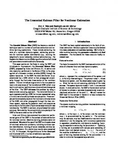
resultant mean and particularly the covariance estimates are biased. In such cases, unstable filter performance may result and the linearized functions often have to be linearized again or a higher–order EKF will have to be used (Julier & Uhlmann, 2002). The need to provide the first—and possibly higher–order Jacobian matrices also limits the class of state–space models to which the EKF can be applied (i.e., functions that are differentiable up to the appropriate orders with respect to the states). In contrast to the EKF, the mean and covariance estimates obtained using the unscented Kalman filter (UKF) proposed by Julier et al. (1995) is at least accurate up to the second (i.e., quadratic) order. It is well proven that the UKF algorithm we describe in the forthcoming section leads to higher estimation accuracy than a first–order EKF. We therefore refer the reader to the work of Julier and colleagues (1996) for a detailed analytic proof, and to extensive simulation results published elsewhere (Van der Merwe et al., 2000; Wan & Van der Merwe, 2001; Nørgaard, Poulsen, & Ravn, 2000; Sitz, Kurths, & Voss, 2002) instead of providing further simulation results here. Of course, we emphasize that the EKF remains a benchmark filter because of its straight–forward relatedness to the linear KF. In many instances, it still serves as the crux of other add–on functions to collectively constitute newer, more robust filtering or smoother techniques (e.g., Molenaar & Newell, 2003; Ghahramani & Roweis, 1999). Unscented Kalman Filter (UKF) The essence of the unscented Kalman filter (UKF; Julier et al., 1995) can be summarized briefly as follows. For each measurement occasion t, a set of deterministically selected points is used to approximate the distribution of the previous state estimates from time t − 1 using a normal distribution with a mean of ηt−1|t−1 , and variance proportional to the state covariance matrix, Pt−1|t−1 . These points, termed sigma points, are specifically selected to capture the dispersion around ηt−1|t−1 . These sigma points are then projected forward in time using the nonlinear dynamic function in Equation 14 and weighted after the transformation to yield ηt|t−1 and Pt|t−1 . Then, the same sigma points are projected using the measurement function in Equation 15, reweighted, and used to update the estimates in conjunction with the new observation at time t to yield ηt|t and Pt|t . In general, both the EKF and the UKF use gaussian approximations to represent the prior and posterior densities of the latent states (i.e., p(ηt |y1:t−1 , θ) and p(ηt |y1:t , θ), respectively). Unlike the EKF, however, the UKF also captures the dispersion in the prior and posterior densities accurately (see Figure 1). The additional scaling constants proposed later by Julier and Uhlmann (2002) can also be used to accommodate slight deviations from normality— namely, to reconstruct symmetric densities with higher or smaller kurtosis (i.e., with fatter or longer tails) than a Gaussian distribution. The abovementioned sigma–point transformation algorithm, capitalized on repeated applications of a transformation technique known as the unscented transformation, is computationally efficient. This is because the sigma points are selected according to a deterministic scheme (instead of a random sampling scheme as in Markov chain Monte Carlo; see e.g., Arminger98a). Further details pertaining to the UKF are summarized below in five major steps (Julier & Uhlmann, 2002; Wan & Van der Merwe, 2001). For ease of presentation, we omit subject index i from our outline below but note that we are still considering the general case wherein parameters are allowed to be time–varying but invariant across


10

Figure 1. A conceptual comparison between the EKF and the UKF. (A) The EKF approximates the prior and posterior distributions of states at each time step by using Gaussian distributions. Because all but the linear terms from Taylor series expansion are ignored, this approach does not always capture the variance of the distribution correctly. Sequential approximations of the nonlinear dynamic and measurement functions by using first–order linear approximations also lead to lower estimation accuracy in cases involving high linearities. (B) The UKF approximates the prior and posterior densities at each time step by using Gaussian distributions created using sigma points (represented as unfilled circle). Because this approach correctly captures the mean, as well as the variance of the state variables before the nonlinear transformation, it also captures the posterior mean and variance correctly through the weighted mean and variance of the post–transformation sigma points.


11

subjects, and states are allowed to vary over time as well as over subjects. We present the UKF algorithm in relation to a computationally simpler subclass of state–space models with additive process and measurement noises also assumed in the case of the EKF. This model is expressed as ηt|t−1 = f (ηt−1 ) + ζt and yt = h(ηt ) + ²t .

(20) (21)

In cases with non–additive noises (e.g., if the noise terms actually appear as part of f [.] or h[.]), additional sigma points will have to be used to approximate the distributions around the current noise estimates. In models with additive noises, the number (and thus computational costs) of the sigma points is reduced substantially. Derivation for these estimates is illustrated in more detail in Julier and Uhlmann (2002) and a summary of the UKF algorithm with non–additive noise is detailed in Wan and Van der Merwe (2001). Step I: Selecting sigma points. Given a w× 1 vector of latent states, a set of 2w + 1 sigma points is selected as χ0,t−1 = ηt−1|t−1 ,

(22)

χk,t−1

(23)

χk,t−1

q = ηt−1|t−1 + [ (w + λ)Pt−1|t−1 ], k = 1, . . . , w q = ηt−1|t−1 − [ (w + λ)Pt−1|t−1 ], k = w + 1, . . . , 2w,

(24)

where w is again the dimension of η 3 . The term λ is a scaling constant composed of two user–specified constants, written as λ = α2 (w + κ) − w

(25)

The UKF is at least accurate up to the second order but biases in higher order terms are scaled by these constants. In cases where prior knowledge of the skewness and kurtosis of the state distribution is known, this information can be further utilized to specify the scaling constants in Equation 25. The constant α is a value between .0001 and 1 that determines the spread of the sigma points away from ηt−1|t−1 . Thus, α can be used to control the amount of higher–order nonlinearities in the vicinity of ηt−1|t−1 that one wants to take into account. If the sigma points are specified to be very close to ηt−1|t−1 , more of the higher–order nonlinearities are ignored. The constant κ is a positive constant used to scale the kurtosis of the sigma point distribution when desired. In practice, the value of κ is not critical and it is usually set to 0, or to 3 - w to ensure that the kurtosis of the sigma point distribution agrees with the kurtosis of a Gaussian distribution (Julier & Uhlmann, 2002; Wan & Van der Merwe, 2001). Step 2: Nonlinear transformation of sigma points through dynamic function. After these sigma points have been selected, each of them is propagated forward in time through the dynamic equation as 3 Note that half of the sigma points are placed to the left of the previous estimate ηt−1|t−1 , and the other half to its right. Thus, the sigma–point index k goes from 1 . . . w, and w + 1 . . . 2w.


χ∗k,t|t−1 = f (χk,t−1 ).

12

(26)

. Step 3: Compute prior state and covariance estimates for latent states. Prior state estimates (i.e., ηt|t−1 ) and covariance estimates (i.e., Pt|t−1 ) at time t are approximated by the weighted mean and variance of the transformed sigma points. Defining a set of weights for the sigma points as (c)

W0

(m)

W0

(c)

Wk

λ + 1 − α2 + β for k = 0, w+λ λ = + 1 − α2 + β, for k = 0 and w+λ 1 (m) = Wk for k > 0. 2(w + λ) =

(27) (28) (29)

The prior state and covariance estimates are then computed using the sigma points and their associated weights as

ηt|t−1 = Pt|t−1 =

2w X

(m)

Wk

χ ∗k,t|t−1 and k=0 (c) Wk [(χk,t|t−1 − ηt|t−1 )(χ ∗k,t|t−1

(30) −ηt|t−1 )0 + Ψ],

(31)

where β is another scaling constant used to incorporate prior knowledge of the distribution of η in the state prediction and update. For Gaussian distributions, β = 2 is optimal (c.f., Van der Merwe et al., 2000). In short, the prior state estimates ηt|t−1 are derived from a weighted mean of the sigma points from step 2, and the prior covariance matrix Pt|t−1 is estimated as the weighted sum of the squared distances of all the sigma points from ηt|t−1 . Step 4: Transformation of sigma points through measurement function. In a similar way, we derive predictions for the manifest observations by subjecting the sigma points to the transformation dictated by the measurement function. More specifically, the predicted measurements and their estimated covariance matrix are generated by first augmenting the prior state sigma–point set (i.e., χ∗k,t|t−1 ) to include the uncertainty constituted by the process noise as √ √ χk,t|t−1 = [χ ∗k,t|t−1 ; χ ∗k,t|t−1 +λ Ψ; χ ∗k,t|t−1 −λ Ψ],

(32)

and subsequently projecting the concatenated sigma–point set through the measurement function as Yk,t|t−1 = h(χk,t|t−1 ).

(33)

Predicted observations and the associated variance and covariance matrices are computed as


yt|t−1 =

2w X

(m)

Wk

Yk,t|t−1 ,

13

(34)

k=0

P yt = P ηt , yt =

2w X k=0 2w X

(c)

(35)

(c)

(36)

Wk [(Yk,t|t−1 − yt|t−1 )(Yk,t|t−1 − yt|t−1 )0 ] + Θ Wk [(χk,t|t−1 − ηt|t−1 )(Yk,t|t−1 − yt|t−1 )0 ].

k=0

Because of the additive process noise, the uncertainty constituted by the process noise can be temporarily “dissociated” from the dynamic process and added after the transformation f [.]. Otherwise, sigma points constructed around the current process noise estimates will have to be propagated through f [.] with the state sigma points (i.e., χk,t−1 in Equation 26) in step 2 as well. The same rules apply here to the additive measurement noise. Step 5: Defining and executing the Kalman filter function. With output from step 4, actual observations are finally brought in and the discrepancy between model prediction and actual observations (i.e., the one–step ahead prediction error) is weighted by a Kalman gain function to yield posterior state and covariance estimates as Kt|t = P ηt , yt P yt−1 , ηt|t = ηt|t−1 + Kt|t (yt − yt|t−1 ), Pt|t = Pt|t−1 −

0 Kt|t P yt Kt|t ,

(37) (38) (39)

where the element P ηt , yt in Equation 37 is also present in the linear case as Pt|t−1 Λ0t (see Equation 7) but was omitted earlier for the sake of clarity. The covariance update function in Equation 39 is formulated in a different but equivalent form than that in Equation 9 to indicate more clearly how the state covariance matrix is updated using output from the sigma–point transformations (Wan & Van der Merwe, 2001). Step 1 to step 5 are then repeated until all the observations have been incorporated. A conceptual summary of the UKF is presented graphically in Figure 2. Approximating Likelihood Using Output from the UKF In order to use maximum likelihood to estimate parameters for nonlinear state–space models with (possibly) non–Gaussian noises, a likelihood function that takes into account the appropriate time dependencies in the data has to be formulated as (Doucet, 1998; Kitagawa, 1998)

L(θ) = p(y1 , . . . , yT |θ) =

T Y t=1

p(yt |y1 , . . . , yt−1 , θ),

(40) (41)


Figure 2. A conceptual representation of the unscented Kalman filter (UKF).

14


15

where p(yt |y1 , . . . , yt−1 , θ) is the conditional density of yt given all the observations from y1 to yt−1 . Due to the dependencies between yt and ηt , p(yt |, y1 , . . . , yT , θ) is obtained by taking into consideration (i.e., integrating over) all possible values of latent states ηt from the joint distribution of ηt and yt as Z p(yt |y1 , . . . , yT , θ) =

p(yt , ηt |y1 , . . . , yt−1 , θ)dηt ,

(42)

p(yt |ηt , θ)p(ηt |y1 , . . . , yt−1 , θ)dηt .

(43)

Z =

In the linear case, the component p(ηt |y1 , . . . , yt−1 , θ) can be readily obtained using the linear Kalman filter4 . Using the UKF, this component is obtained by means of Gaussian approximations. In certain special cases, the conditional measurement density p(yt |ηt , θ) also has known analytic forms. For instance, under the assumptions of a nonlinear dynamic model with additive process noise and a linear measurement model with additive Gaussian measurement noise, p(yt |ηt , θ) can be expressed as a function a Gaussian density function (for exact form see Doucet, 1998). As we mentioned earlier, in the context of the linear KF, the prediction error decomposition function is used to derive L(θ) based on one–step–ahead prediction errors from the linear KF. These errors can be viewed as discrepancies or new information brought in by current observations and are often termed innovations. Thus, the prediction error decomposition function is referred to as the innovations form of the likelihood function (Shumway & Stoffer, 2004) with associated covariance matrix P yt given by Equation 12. In situations in which the one–step–ahead prediction errors are independently and normally distributed after all the nonlinear dynamic and measurement relations have been accounted for, the UKF provides the one–step–ahead prediction errors and P yt (see Equation 35) which can then be used in conjunction with the prediction error decomposition function to yield approximate ML parameter estimates. Young, McKenna, and Bruun (2001), for instance, used prediction error decomposition in a similar way (but not with the UKF) to estimate parameters for nonlinear stochastic systems. We use the UKF in conjunction with prediction error decomposition in our first illustrative example to estimate time–invariant parameters of the classical predator–prey model with single– and multiple–subject data. In our second illustrate example, we use the UKF to estimate the states and most of the parameters for the Lorenz system, and then use the quasi–ML approach to estimate the process and measurement noise covariances. Parameter estimates obtained in both cases are accurate under assumptions of a linear measurement model with additive and normally distributed process and measurement noises. As the distribution of the prediction errors deviates more from normality (e.g., when the process and measurement noises are not normally distributed, or when higher–order moments are needed to account for the high non–linearities in one’s model), alternative approaches such as particle filters, MCMC methods and gaussian mixture filters can be used. We discuss some of these possibilities in the Discussion section. 4

Note that we do not explicitly specify the lower and upper limits of the integral in Equations 42– 43 because it is implied that the integral is computed over the interval of all possible values of η at time t. The lower and upper boundaries of the interval are thus dependent on the values of ηt .


16

Simulation Examples Classical Predator–Prey Model We used the UKF with prediction error decomposition to fit data simulated using the classical predator-prey model (Lotka, 1925; Volterra, 1926), which is often termed the Lotka–Volterra equation. This model captures the interaction between a predator and a prey population and it is written as x˙1t = r1 x1t − a12 x1t x2t , and

(44)

x˙2t = r2 x2t + a21 x1t x2t ,

(45)

where x1t corresponds to density of the prey population at time t and x2t the density of the predator population. The component x˙qt on the left–hand–side of the two equations thus represents the rate of change in the density of species q. The parameter r1 is used to represent the growth rate of the prey population and r2 is the death rate of the predator population because the latter is hypothesized to decrease in size in the absence of its sole food source (i.e., the prey). Consequently, the interaction between the predator and prey population is hypothesized to lead to negative outcome for the prey population (thus Equation 44 has the component −a12 instead of +a12 ) whereas the predator population is assumed to benefit from this interaction (the magnitude of which is determined by a21 ). Equations 44– 45 are known to yield cyclic fluctuations in predator and prey densities in a lead–lag manner. Alternatively, x1t and x2t may represent a person’s scores on two tests, one of which is hypothesized to be positively moderated by the other, and the other one is negatively moderated by the first test. An extended version of this model was used by Chow and Nesselroade (2004) to represent age differences in susceptibility to interference. Suppose we have data from 200 pairs of different predator–prey species and wish to deduce a common trend that is invariant across all species. To formulate multiple–species or multiple–subject predator–prey model as a discrete–time state–space model, we express the dynamic and measurement models as · ¸ · ¸ · ¸ xi1t f1 (xi1,t−1 , xi2,t−1 , θ) ζ = + i1t and xi2t f2 (xi2,t−1 , xi2,t−1 , θ) ζi2t

(46)

      ²i1t 1 0 yi1t ²i2t  λ21 0  yi2t  ·    ¸       yi3t    = λ31 0  x1it + ²i3t  ²i4t    0 yi4t  1  x2it      ²i5t   0 λ52  yi5t  ²i6t 0 λ62 yi6t

(47)

where xi1t and xi2t are person i’s true underlying attributes apprehended respectively through the indicators yi1t —yi3t and yi4t —yi6t . ζiqt (q = 1, 2) represents the process noise that influences person i’s true attribute q at time t, ²ijt represents the measurement error


17

associated with person i’s score on test j at time t, λjq is the factor loading of indicator j on attribute q and θ is a set of time–invariant parameters to be estimated (including r1 , r2 , a12 , a21 and process and measurement noise covariance matrices Ψ and Θ). The term fq (.) represents discrete approximations to the differential equations in 45– 46 by means of a fourth-order Runge-Kutta approach. A fourth–order Runge–Kutta is a way to obtain numerical integral solution to a set of differential equations. This is done by first deducing changes at four arbitrarily small intervals between two successive measurement occasions based on the dynamic functions, and subsequently computing the value of xiq at time t by smoothing over these changes. As the computation intervals become very small, a smooth, continuous trajectory results (for implementation details see Press, Teukolsky, Vetterling, & Flannery, 2002). In this way, a discrete trajectory is mapped onto a continuous trajectory by smoothing over the “missing observations” that exist between two measurement intervals. Note that the classical predator–prey was originally formulated as a deterministic model (i.e., there is no process noise; see Equations 44– 45). For illustration purposes, we set Ψ to be a diagonal matrix with very small process noise variances. We simulated data using true parameters in Table 1 with (1) a single time–series with N = 1 and T = 200 and (2) multiple–subject data with N = 200 and T = 50. Results from model fitting are summarized in Table 1. Standard errors associated with the parameter estimates were obtained by computing the finite difference Hessian matrix evaluated at the final parameter estimates. In the case of multiple–subject data, the UKF procedures were performed sequentially from time t = 1 to T , and for person i to N . We then used a minimization function in Matlab called fminsearch to minimize −LLK F (θ) in Equation 13 iteratively until the changes in fit function in successive iterations are smaller than an arbitrarily small value. 5 To create a more realistic scenario, we gave all the fictitious participants in our multiple–subject case different initial scores at time 1 (specifically, we added a normally distributed error term with a mean of zero and a standard deviation of 5 to the average initial scores). The resultant individual trajectories and aggregate curves are presented in Figure 3. For estimation purposes, each individual’s observed scores on the first measurement occasion were uset to set their initial conditions and the initial state covariance matrix was set to be a diffuse diagonal matrix with variances of 100. As shown in Table 1, parameter estimates converged satisfactorily to the true values in both the single time series and multiple–subject cases. As is typical in most cases involving ML–estimation of more complex nonlinear models, computational time was rather long, especially in the multiple–subject case (see footnotes in Table 1). Even though 50 measurement occasions may seem like a luxury for typical applications in social sciences, we note that only two complete cycles of oscillation were available for model estimation from each individual. This is because the dynamics of the predator– prey system evolve relatively slowly over time at our specific choice of parameters (see Figure 3). Researchers should therefore bear in mind the nature of the dynamics they intend to capture (e.g., daily cycles, weekly cycles and so on) and subsequently sample both within and across successive cycles. Practically speaking, it is possible to analyze a 5

Specifically, all the subtraction signs in Equation 13 have to be replaced with summation signs to yield the corresponding negative log–likelihood function which one can then minimize instead of maximize with respect to the parameters.

18


large sample of individuals with shorter data segments (i.e., panel data with smaller T ) using the techniques presented herein. However, if inter–individual differences exist in the parameters (and hence, dynamics), including more individuals in the sample and analyzing them as an aggregate does not really help in improving estimation accuracy. Sufficient measurement occasions are still needed within a person to effectively identify within–person changes. Thus, panel data are helpful for identifying inter–individual differences in change (see e.g., the SEM–based state–space modeling approach presented by J. H. L. Oud & Jansen, 2000). However, when one’s focus is on identifying intraindividual changes, and individuals in a sample indeed differ in their respective behavioral dynamics, one then lacks enough information to untangle more complex (e.g., nonlinear) within–person changes from interindividual differences. In contrast, data with large N and T ≥ 50 are becoming more prevalent in the social sciences with the increased popularity of experience sampling studies (e.g., Diener, Fujita, & Smith, 1995). We therefore chose this design as an illustrative case. Table 1: True parameters used to simulate the classical predator–prey model and parameter estimates from model fitting. Standard errors are included in parentheses.

Parameters

True values

(A) UKF estimates with a

r1 r2 a12 a21

Λ

Ψ

Θ

4.0 3.0 .8 .5   =1 0  .9 0     .7 0     0 = 1    0 .8  0 · 1.2 ¸ .0001 diag .0001   15 15   15  diag 7   7 7

a b

N = 1, T = 200 3.843 (.003) 3.133 (.003) .805 (.001) .487 (.014)   =1 0 .760(.043)  0   .638(.026)  0     0 =1    0 .832(.022)  0 · 1.356(.014) ¸ .011(.009) diag −.001(.000)   14.137(.677) 15.608(.936)   11.995(.862)   diag    6.953(.586)   5.899(.178)  8.399(.265)

(B) UKF estimates with N = 200, T = 50 b 4.146 (.082) 2.602 (.041) .770 (.017) .479 (.005)   =1 0 .978(.010)  0   .766(.008)  0     0 =1    0 .770(.005)  0 · 1.160(.006) ¸ .013(.001) diag .075(.002)   18.952(.319) 18.131(.296)   13.926(.182)   diag   9.356(.179)   6.473(.089)  6.942(.102)

Estimation procedure took 7.52 minutes of CPU time on a 2 GHz IBM laptop with 1 GB RAM. Estimation procedure took 14.54 hours of CPU time on a 2 GHz IBM laptop with 1 GB RAM.

The Lorenz system We now present simulation results based on the Lorenz system (Lorenz, 1963), a well– known dynamical system that exhibits chaotic dynamics and properties such as sensitive

19


25 Average predator density

Population densities

20

Average prey density

15 10 5 0

−5 −10 0

10

20

30

40

50

Time Figure 3. Individual trajectories and aggregate curves of the classical predator–prey system. This system is known to show ongoing lead–lag fluctuations in densities over time.


20

dependence on initial conditions6 —or the“butterfly effect”. We used a single time–series with intensive repeated measures (T = 2000) and used a joint estimation approach with the UKF to estimate the parameters as states. Although this type of data is relatively uncommon in the social sciences, such data sets are very prevalent, for instance, in physiological, Electro-Encephalography (EEG) and perceptual-motor studies. Originally used to represent the weather system, the Lorenz system comprises three latent state variables (denoted below as x1t , x2t and x3t ), the dynamics of which are expressed as x˙1t = σ(x2t − x1t ),

(48)

x˙2t = ρx1t − x2t − x1t x3t and

(49)

x˙3t = x1t x2t − βx3t ,

(50)

where the system as a whole is used to describe the convection flow within a layer of air (or the motion of a fluid within a container) being heated from below and cooled from above, with both ends kept at constant temperatures. Due to temperature differences at both ends, warm air rises and cool air sinks. In this case, x1t represents the convective flow of the air at time t, x2t the horizontal temperature distribution at time t and x3t the vertical temperature distribution at time t, σ the ratio of viscosity to thermal conductivity, ρ is the temperature difference between the two ends of the layer, and β is the width–to–height ratio of the layer (Alligood et al., 1996). These variables and parameters combined provides a simple description of the atmosphere—air at the bottom is heated by the earth and the top is kept cooled by the void of outer space. The Lorenz equations have been used to describe the ongoing “tension” between an individual’s positive affect and negative affect (Frederickson & Losada, in press). At the specific parameters of σ = 10, ρ = 46 and β = 8/3, the convection flow exhibits chaotic patterns that seem to be repeating themselves (i.e., self–similar) over time; yet, the exact numerical values of the states can be very different with just slight differences in initial conditions. Frederickson and Losada (in press) argued that individuals who have such a “chaotic” emotional profile are associated with higher emotional complexity and psychological resilience. We generated data using the parameter values outlined above with no process noise7 , with each latent variable identified by one indicator that is corrupted with measurement noise at approximately 70% signal–to–noise ratio. A plot of the clean time series is shown in Figure 4. The three state variables of the Lorenz system can be observed to show seemingly random and yet, self–similar (or self–repetitious) behaviors over time. Pairwise plots of the noisy observations used to identify the latent latent variables are shown in Figure 5. As evidenced in Figure 5, the true dynamics among the three state variables are completely masked. Using a joint estimation approach, we represent σ, ρ and β as part of the state vector xt = [x1t , x2t , x3t , σt , ρt , βt ]0 and estimate their values using the UKF in conjunction with x1t , x2t and x3t . The corresponding dynamic model is written as 6

This is the property that slight differences in initial conditions could lead to cascading divergence in later dynamics. 7 Chaotic systems are known to be nonlinear dynamical systems that are deterministic and yet manifest seemingly random behaviors.

21


60 x1 t x2 t x3

50

t

40

States

30 20 10 0 −10 −20 −30 0

500

1000

Time

1500

2000

Figure 4. A plot of the clean dynamics of the Lorenz system. The three latent variables show seemingly random but self–similar long–term behaviors. We included more measurement occasions on purpose to illustrate this property more clearly.

22


40

60

30

50

20

40

10

30

y3t

70

y2t

50

0

20

−10

10

−20

0

−30

−10

−40 −50

0

y1t

50

−20 −50

0

y1t

50

Figure 5. Pairwise plots of the corrupted time series against each other. The true relationships among the latent variables are completely masked by measurement noise.


    x1t f1 (xt−1 ) x2t  f2 (xt−1 )     x3t  f3 (xt−1 )   =    σt   σt−1  ,      ρt   ρt−1  βt βt−1

23

(51)

where fq (xt ), (q = 1, 2, 3) is again the numerical solutions to Equations 48— 50 obtained by means of a fourth–order Runge–Kutta integration. The corresponding measurement model is written as  1 0    y1t  y2t  = 0 0  y3t 0 0

0 1 0 0 0 0

0 0 1 0 0 0

0 0 0 0 0 0

0 0 0 0 0 0

  0 x1t     0  x2t  ²1t   0  x3t  + ²2t  .   0   σt  ²3t  0  ρt  βt 0

(52)

Although the parameters do not vary over time, we incorporate them into the time– varying state vector and subsequently constrain them to be invariant over time8 . As such, time–varying parameters can be estimated easily using this approach (for examples on time–varying models see e.g., Harvey, 1989; Kim & Nelson, 1999). For instance, one can hypothesize that certain parameters in a model actually follow a first–order autoregressive process (i.e., a random walk model) instead of being constant over the entire span of a study. Within-person deviations in parameters (e.g., slope of a growth curve) are rarely examined in many empirical studies but this kind of “non–stationarity” may have important implications for various developmental and psychological phenomena. For instance, discontinuity in development as posited by Piaget’s stagewise developmental model and related catastrophe models (Van der Maas & Molenaar, 1992) can also be handled more easily using this approach. Here, we estimated σ, ρ and β as part of the state vector using the UKF. We used approximate–ML with prediction error decomposition to estimate the measurement error variances (²1t —²3t ). Compared with the approximate–ML approach we used in the predator–prey example to estimate all parameters, the reduction in computational time can be rather substantial (i.e., from days to minutes or hours). Based on our past experience, separating the estimation of the states and other parameters from estimation of elements of Ψ and Θ generally leads to more numerically stable and accurate results. Using other mechanisms to estimate the time–invariant noise matrices is beneficial because noise variances are used to determine the spread of the sigma points from one’s current estimates in the UKF. This is less of an issue in many applications in the physical sciences because the UKF is typically used in cases wherein values of process noise and measurement noise covariance matrices (Ψ and Θ, respectively) are known. 8 Alternatively, a separate UKF chain can be run to estimate the parameters, again by treating them as state variables. This is the dual Kalman filter approach mentioned earlier.

24


Table 2: True parameters used to simulate the Lorenz system and parameter estimates recovered by a joint state–parameter estimation approach using the UKF. Prediction error decomposition was only used to estimate the measurement error variances. Standard errors are included in parentheses.

Parameters σ ρ β Θ a

True values 10 28 2.667   26  diag 34 32

UKF estimates with joint state–parameter estimation procedures (N = 1, T = 2000) 9.544 (.095) 27.916 (.090) 2.524  (.016)  25.78(.291)  diag 31.23(.345) 28.53(.377)

a

Estimation procedure took 8.97 minutes of CPU time on a 2 GHz IBM laptop with 1 GB RAM.

Final parameter estimates are summarized in Table 2. The three parameter estimates converged to the true values after approximately 1000 measurement occasions. State estimates recovered by the UKF also reproduced the true dynamics among the latent variables in the form of a strange attractor very accurately (see Figures 6A—D). Here, the state variables manifest very complex time–based dynamics (see Figure 4), but they maintain lawful relationships with one another. Even though slight differences in initial conditions can lead to great divergence in later numerical values of the states , the overall “shape” of the butterfly–like attractor is always maintained—hence the name strange attractor. Additional approaches can be used to help tune the parameter estimation process to lead to faster convergence but we did not use such methods here. With appropriately tuned filter, Sitz et al. (2002), for example, reported convergence of the parameter estimates from the Lorenz system to their true parameter values with less than 300 measurement occasions and 50% signal–to–noise ratio. A common “trick” to speed convergence is to add a a small amount of process noise variances to the parameters (which in this case was specified to be deterministic process noises with zero process noise variances). This approach helps prevent the parameter estimates from lingering in local minima for a long time, and was adopted by e.g., Molenaar and Raijmakers (1998). Similar approaches for shaping the process noise of the parameters are detailed in Wan and Van der Merwe (2001). Standard error estimates for parameters estimated using the UKF were obtained from the square–root of the state covariance matrix (Pt|t ) (Sitz et al., 2002). Here, the standard error estimates were slightly underestimated and this situation often arises when the parameter estimates stabilize too early on in the estimation process. Further research into ways to resolve this issue more effectively is certainly warranted.

An Empirical Example of Dyadic Interactions in Emotions Within the context of dyadic interactions, dynamic systems models have inspired new ways of conceptualizing the dynamics within dyads. Felmlee and Greenberg (1999), for instance, used a set of linear differential equations to represent spouses’ differing goals, preferences or ideals, and how both parties may compromise and settle into an equilibrium over

25


40

60

(B)

(A) 40

xhat1t

xhat1t

20 0

20

−20

0

−20

0

20

−20

xhat2t

40

20

xhat3t

60

(D)

(C) 40 x

1t

20 x1t

0

0

−20 −20

20 0

0

x2t

20

−20

0

x3t

20

Figure 6. (A) and (B): Plots of the state estimates recovered using the UKF; (C) and (D): Plots of the clean state variables over all time points. True dynamics among the state variables are accurately recovered by using the UKF


26

time. Gottman and colleagues (Gottman, Murray, Swanson, Tyson, & Swanson, 2002) have also used nonlinear dynamic models to represent emotional interaction between spouses and to predict marital success. The dynamic interplay between positive and negative emotions within and across different individuals thus captures the possibility that increases in negative emotion during certain life periods might be moderated by increases or maintenance of positive emotion during the same periods, as predicted, for instance, by Carstensen’s (1993) theory of socioemotional selectivity. We examined a specific kind of interactive dynamics between positive and negative emotions by fitting the classical predatory-prey model to a set of affective ratings from one married couple. Positive and negative emotions were measured using the Positive and Negative Affect Schedule (PANAS; Watson, Lee, & Tellegen, 1988) over 182 consecutive days. Linear lagged relationships between the couple’s positive affect and negative affect have been examined elsewhere (Ferrer & Nesselroade, 2003), and the husband’s negative affect (NA) was found to have a lagged effect on the wife’s positive affect (PA) and negative affect (NA), but not the other way around. Here, we modeled the interaction between the couple’s affect with the husband’s NA serving as a “predator” and the wife’s PA as a “prey” (Model 1). We then reversed the role of the couple and represented the wife’s NA as a predator and the husband’s PA as a prey (Model 2). We consolidated data from the original 20-item PANAS by using item parceling (Kishton & Widaman, 1994) and used three PA item parcels to identify each person’s PA, and three NA item parcels to identify each person’s NA. Table 3: Parameter estimates obtained from fitting the predator–prey model to the wife’s PA ratings and the husband’s NA ratings. Three PA parcels and three NA parcels were used to identify the wife’s PA and the husband’s NA, respectively.

Model

Parameters

Estimates

Model 1: Wife’s PA as prey and husband’s NA as predator

rwif eP A rhusbandN A ahN A−→wP A awP A−→hN A λ11 λ21 λ31 λ41 λ52 λ62

3.01 (.006) 5.91 (.005) 1.07 (.001) .31 (.002) =1 .69 (.041) .74 (.050) =1 .70 (.067) 1.03 (.103)   8.94(.168) 6.69(.293)   7.52(.396)   diag  4.03(.130)   3.44(.173) 6.02(.266)

Θ

We rescaled the affect ratings by subtracting them from 1 (thus a zero rating corre-

27


Table 4: Parameter estimates obtained from fitting the predator–prey model to the husband’s PA ratings and the wife’s NA ratings. Three PA parcels and three NA parcels were used to identify the husband’s PA and the wife’s NA, respectively.

Model

Parameters

Estimates

Model 2: Husband’s PA as prey and wife’s NA as predator

rhusbandP A rwif eN A awN A−→hP A ahP A−→wN A λ11 λ21 λ31 λ41 λ52 λ62

3.86 (.161) 1.20 (.025) 3.80 (.228) .06 (.000) =1 .93 (.031) 1.31 (.039) =1 2.48 (.278) 3.29 (.324)   5.71(.157) 5.94(.212)   6.89(.241)  diag 1.86(.103)   3.59(.203)

Θ

4.14(.229)

sponds to an original score of 1, which was measured on a scale of 1 to 5), and multiplying the resultant scores by 10 because of the dyad’s general low variability in negative emotion. Results from model fitting are summarized in Tables 3— 4. Parameter estimates in both models were reliably different from zero. Note that the process noise covariance matrix, Ψ, was set to a null matrix and was not estimated. This was because the classical predator–prey model was originally formulated as a deterministic model with no process noise. In situations with low affect scores, even a slight amount of process noise can lead to negative affect scores (i.e., negative species density). Scenarios with negative densities, however, are not justifiable from a predator–prey standpoint and are thus not considered here. We also note that model fit statistics can be obtained directly from the prediction error decomposition function in Equations 13 (i.e., by computing LLKF [θ]) Harvey, 1989), but more extensive simulation studies are needed to establish the feasibility of using such fit statistics to evaluate the fit of nonlinear dynamic models. Whereas both individuals’ PA was, to a certain extent, “encroached” by the other person’s NA, the husband’s PA was more negatively affected. In addition, although the husband’s NA increased slightly as a result of “interacting” with the wife’s PA, his NA decayed much more rapidly at baseline compared with the wife’s NA. In contrast, the wife’s increase in NA due to interaction with the husband’s PA was almost negligible. Expected trajectories generated using parameter estimates from model fitting are shown in Figures 7A–B. Note that in both models, magnitudes of the dyad’s PA ratings were greatly overestimated. This was due in part to the fact that the dyad’s NA died out pretty quickly and was generally maintained at extremely low levels (near zero). Thus, according


28

to the prediction of the classical predator–prey model, the dyad’s PA should grow without boundary in the absence of the other partner’s NA. Taken together, individuals’ PA may not be well characterized by the classical predator-prey model (e.g., some upper limits would have to be imposed). The dyad’s fluctuations in NA, in contrast, were well captured by the dynamics of the predator. In successful emotion regulation scenarios, it is reasonable to expect one’s NA to decay or die out naturally in the absence of further external influences— this is evidenced in the actual data as well as in the expected trajectories of NA. In sum, our current findings extend Ferrer et al.’s (2003) earlier finding concerning the unidirectional effect of husband’s affect on wife’s affect in that we found bidirectional influence in the dyad—but in the more subtle way of an interaction effect between PA and NA. Thus, by providing an empirical example of dyadic interaction, we showed how one variation of UKF can be used to discern the dynamics of affect interrelations between spouses, as their affects evolve co-dependently over time. A similar approach can be used to examine the development of emotional interactions between a child and a caregiver, as posited by attachment theory (Bowlby, 1969/1982), or the emotional co-regulation between two individuals in a close relationship (e.g., Gottman et al., 2002; Thompson & Bolger, 1999).

Discussion Dynamical systems, as defined earlier, are systems whose current states are somehow dependent on their previous states. The basic ideas have clearly “struck a chord” with behavioral scientists interested in process and other kinds of change. Over the last few decades, however, some of the initial enthusiasm for nonlinear dynamical systems has turned into reserved speculation, if not total disenchantment with the applicability of dynamical systems–related ideas to psychological research. A large part of this disappointment stems from the unrewarded investment of many researchers in chaotic systems, including the Lorenz system used in one of our simulation examples. In their comments on the current status of chaotic analysis in psychology and psychoanalysis, Kincanon and Powel (1995) noted that applications of chaos in psychology are often limited to two broad categories: “chaos as a mathematical model of psychological phenomena and chaos as a metaphor for psychological phenomena” (p. 1). Developing and evaluating estimation techniques that allow a direct mapping between more complex mathematical models of change and empirical measurements is therefore an important step toward revoking the belief that chaos is strictly a theoretical metaphor in social and behavioral research. In the present context, we demonstrated the generality and flexibility of the nonlinear state-space modeling framework in fitting dynamic models. The relative ease of using Kalman filter methods to estimate time-varying parameters is also an important model– fitting feature. In models of social interaction, for example, parameters may change as a result of contextual influences, developmental changes, or changes elicited by specific reactions from a spouse (e.g., sudden transition from a predator-prey relation to a cooperative relation). Especially pertinent are nonlinear and catastrophe-based developmental models that are theoretically grounded but are difficult to fit using conventional modeling tools (e.g., Van der Maas & Molenaar, 1992) because the changes in states depend on the changes in parameters within a system. Adding to this advantage is the Kalman filters’ overall efficiency and ease of implementation.

29


9 8

(A)

wife E[PA] husband E[NA] wife observed PA husband observed NA

Affect intensity

7 6 5 4 3 2 1 0

50

100

150

Day 9 8

(B)

husband E[PA] wife E[NA] husband observed PA wife observed NA

Affect intensity

7 6 5 4 3 2 1 0

50

100

150

Day Figure 7. Actual affect ratings and expected trajectories generated using parameter estimates from model fitting with (A) Wife’s PA as the prey and husband’s NA as the predator and (B) husband’s PA as the prey and wife’s NA as the predator.


30

Several recent developments in fitting nonlinear, non–Gaussian state–space models are worth mentioning here. The major estimation problem central to all nonlinear, non– Gaussian state–space models is essentially the need to deal with non–Gaussian distributions (e.g., posterior density of states, p[ηt |yt , θ], transition density, p[ηt |ηt−1 , θ] and likelihood functions, p[yt |y1 , . . . , yT , θ]). At times, the distributions involved are multi–modal and do not have known analytic forms. In such cases, the prediction error decomposition function can no longer be used. One possibility for approximating such multi–modal distributions is to use a class of sequential Monte Carlo techniques collectively known as particle filters (Doucet, de Freitas, & Gordon, 2001). One of the earliest versions of such particle filter approaches is the bootstrap filter proposed by Gordon, Salmond, and Smith (1993). Instead of attempting to sample from analytically intractable distributions (that might even be difficult to approximate via simulation techniques), the approach taken here is to generate a large number of points or particles from an alternative distribution from which one can easily sample. These particles are then weighted and the associated weights can be used to approximate non–normal prior and posterior densities (e.g., Kitagawa, 1998), as well as likelihood functions (e.g., Pitt, 2002). Thus, instead of running one UKF chain, for example, multiple UKF chains are run using these particles (e.g., Van der Merwe et al., 2000). In practice, particle filter techniques are often used in conjunction with Markov chain Monte Carlo methods (e.g., Van der Merwe et al., 2000) to improve their respective estimation accuracy. Interested readers are referred to Doucet et al. (2001) for a collection of such methods (see also Durbin & Koopman, 2001; Shumway & Stoffer, 2004). A related line of work on fitting nonlinear state–space models stems from the earlier Gaussian sum filter approach proposed by Sorensen and Alspach (1971). This particular approach involves approximating non–Gaussian densities using a mixture of different Gaussian densities. Similar approaches are commonly adopted in the social sciences for approximating non–Gaussian densities in nonlinear cross–sectional models (e.g., Klein & Moosbrugger, 2000) and other mixture modeling approaches (e.g., McLachlan & Peel, 1995), but less so within the context of dynamic model fitting. Although Gaussian sum filters and other newer Monte Carlo variations of these filters (e.g., Liu & West, 2001) bring with them other methodological challenges (e.g., to estimate the number of mixture components from occasion to occasion), much can be gained from this kind of filtering or smoothing techniques because they were developed to fit dynamic models—a much needed class of modeling tools in social sciences. In addition, these techniques are just as well suited for estimating parameters or factor scores in the special case of nonlinear cross–sectional models. Most often, only trivial modifications are needed. To make the fitting and evaluation of non-linear dynamical models to behavioral data a practical activity, much remains to be done. We hope to have introduced the reader to some useful contemporary techniques in estimating nonlinear dynamical systems. However, we emphasize that this is just the beginning, not the end to the modeling work in this area. Much research still needs to be done to improve the convergence speed of the aforementioned model fitting techniques, and to derive more practical standard error estimates and fit statistics for model comparison purposes. Admittedly, all our simulation and empirical modeling examples were based on rather intensive repeated measurements by the standards of most applications in social sciences. As we have alluded to earlier, the confounds between interindividual differences and intraindividual change—including intraindividual


31

fluctuations from occasion to occasion—are especially difficult to disentangle in the case of nonlinear dynamic models. For one, all the individual cases in our multiple–subject example were designed to have the exact same parameters (including noise covariance matrices). In situations wherein the parameters actually differ across individuals (e.g., for evaluating nonlinear dynamic models with mixed effects), more measurements are needed from each individual. In fitting chaotic models, for instance, the property of sensitive dependence on initial conditions can lead to complex, cascading between–person differences in state dynamics. In our view, including more repeated measurements within and across different individuals is simply a “safer” route because it provides the researcher with more options for representing within–person changes (in states as well as parameters) if he/she so chooses. Taken together, we see these methodological difficulties not so much as a hurdle but more as an even stronger incentive for social scientists to include more intensive repeated measurements in longitudinal designs.

Conclusion As a discipline, psychology has generally seemed reluctant to embrace what Wohlwill (1991) described as a tension between method and theory—for a given period, methodological developments may lag behind theoretical ideas or vice versa, but it is the ongoing tension between the two that helps propel further advances in both method and theory (Nesselroade & Cattell, 1988). Methodological difficulties and naive understanding of the concept of parsimony have fostered a deeply rooted bias against nonlinear models—an unfortunate limit imposed by methodology on theory. Parsimony and convenience, however, should not be the sole reasons for model selections, especially when the nonlinear models under consideration are supported by strong theoretical knowledge. Undoubtedly, several methodological issues remain in evaluating nonlinear, non–Gaussian state–space models. Nonetheless, the Kalman filters’ potential as a dynamic model-fitting tool are evident and, hopefully, can help inspire more research into alternative methods that are suited for the study of change—including both linear and nonlinear dynamic models.

References Alligood, K. T., Sauer, T. D., & Yorke, J. A. (1996). Chaos: An introduction to dynamical systems. New York: Springer-Verlag. Arminger, G. (1986). Linear stochastic differential equation models for panel data with unobserved variables. In N. Tuma (Ed.), Sociological methodology 1986 (pp. 187–212). San Francisco: Jossey–Bass. Arminger, G., & Muthén, B.(1998). A Bayesian approach to nonlinear latent variable models using the Gibbs sampler and the Metropolis–Hastings algorithm. Psychometrika, 63, 271–300. Bereiter, C.(1963). Some persisting dilemmas in the measurement of change. In C. W. Harris (Ed.), Problems in measuring change. Madison, WI: University of Wisconsin Press. Boker, S. M., Neale, M. C., & Rausch, J. (in press). Latent differential equation modeling with multivariate multi-occasion indicators. In H. O. K. van Montfort & A. Satorra (Eds.), Recent developments on structural equation models: Theory and applications (p. 151-174). Amsterdam: Kluwer. Bowlby, J.(1969/1982). Attachment and loss: Vol. 1. attachment (2nd ed.). New York: Basic Books.


32

Carstensen, L.(1993). Motivation for social contact across the life span: A theory of socioemotional selectivity. In J. E. Jacobs (Ed.), Nebraska Symposium on Motivation (pp. 209–254). Lincoln: University of Nebraska Press. Chow, S.-M., & Nesselroade, J. R. (2004). General slowing or decreased inhibition? mathematical models of age differences in cognitive functioning. Journals of Gerontology Series BPsychological Sciences & Social Sciences, 59B (3), 101–109. Coleman, J. S. (1968). The mathematical study of change. In J. H. M. Blaylock & A. Blaylock (Eds.), Methodology in social research (pp. 428–478). New York: McGraw–Hill. Cronbach, L. J., & Furby, L.(1970). How should we measure “change”–or should we? Psychological Bulletin, 74 (1), 68–80. Diener, E., Fujita, F., & Smith, H.(1995). The personality structure of affect. Journal of Personality and Social Psychology, 69 (1), 130–141. Dolan, C. V., & P. C. M. Molenaar. (1991). A note on the calculation of latent trajectories in the quasi markov simplex model by means of regression method and the discrete kalman filter. Kwantitatieve methoden, 38, 29–44. Doucet, A.(1998). On sequential simulation–based methods for bayesian filtering. (Technical Report CUED/F–INFENG/TR.310, Signal Processing Group, Department of Engineering, University of Cambridge.,) Doucet, A., de Freitas, N., & Gordon, N. (Eds.). (2001). Sequential Monte Carlo methods in practice. New York: Springer. Durbin, J., & Koopman, S. J. (2001). Time series analysis by state–space methods. New York: Oxford University Press. Felmlee, D. H., & Greenberg, D. F.(1999). A dynamic systems model of dyadic interaction. Journal of Mathematical Sociology, 23 (3), 155–180. Ferrer, E., & Nesselroade, J. R.(2003). Modeling affective processes in dyadic relations via dynamic factor analysis. Emotion, 3 (4), 344–360. Frederickson, B. L., & Losada, M. F.(in press). Positive affect and the complex dynamics of human flourishing. American Psychologist. Gelb, A., with Technical staff of The Analytic Sciences Corporation. (1974). Applied optimal estimation. Cambridge, MA: MIT Press. Ghahramani, Z., & Roweis, S.(1999). Learning nonlinear dynamical systems using an EM algorithm. In M. Kearns, S. Solla, & D. Cohn. (Eds.), (Vol. 11, pp. 599–605). Cambridge, MA: MIT Press. Gordon, N. J., Salmond, D. J., & Smith, A. F. M.(1993). Novel approach to nonlinear/non–Gaussian Bayesian state estimation. IEEE Proceedings–F, Radar and Signal Processing, 140 (2), 107–113. Gottman, J. M., Murray, J. D., Swanson, C. C., Tyson, R., & Swanson, K. R. (Eds.). (2002). The mathematics of marriage: Dynamic nonlinear models. Cambridge, MA: MIT Press. Haken, H. (1977/83). Synergetics, and introduction: Non-equilibrium phase transitions and self– organization in physics, chemistry and biology. Berlin: Springer–Verlag. Hamblin, R. L., Hout, M., Miller, J. L. L., & Pitcher, B. L.(1977). Arm races: A test of two models. American Sociological Review, 42 (2), 338–354. Hamerle, A., Nagl, W., & Singer, H. (1990). Problems with the estimation of stochastic differential equation using structural equations models. Journal of Mathematical Sociology, 16 (3), 201–220.


33

Hamilton, J. D. (1994). Time series analysis. Princeton, NJ: Princeton University Press. Harvey, A. C. (1989). Forecasting, structural time series models and the Kalman filter. Princeton, NJ: Princeton University Press. Jöreskog, K. G., & Yang, F. (1996). Nonlinear structural equation models: The Kenny–Judd model with interaction effects. In G. A. Marcoulides & R. E. Schumacker (Eds.), Advanced structural equation modeling (pp. 57–88). Mahwah, NJ: Lawrence Erlbaum. Julier, S. J., & Uhlmann, J. K.(1996). A general method for approximating nonlinear transformations of probability distributions. (Technical Report RRG, Department of Engineering Science, University of Oxford) Julier, S. J., & Uhlmann, J. K.(2002). Reduced sigma point filters for the propagation of means and covariances through nonlinear transformation. In Proceedings of the IEEE American Control Conference (pp. 887–892). Anchorage AK, USA: IEEE. Julier, S. J., Uhlmann, J. K., & Durrant-Whyte, H. F. (1995, June). A new approach for filtering nonlinear systems. In Proceedings of the American Control Conference (pp. 1628–1632). Seattle, Washington: IEEE. Kalman, R. E. (1960). A new approach to linear filtering and prediction problems. Transactions of the ASME–Journal of Basic Engineering, 82 (Series D), 35-45. Kaplan, D., & Glass, L. (1995). Understanding nonlinear dynamics. New York: Springer–Verlag. Kenny, D. A., & Judd, C. M. (1984). Estimating the nonlinear and interactive effects of latent variables. Psychological Bulletin, 96, 201–210. Kim, C.-J., & Nelson, C. R. (1999). State-space models with regime switching: Classical and Gibbssampling approaches with applications. Cambridge, MA: MIT Press. Kincanon, E., & Powel, W.(1995). Chaotic analysis in psychology and psychoanalysis. The Journal of Psychology, 129, 495–505. Kishton, J. M., & Widaman, K. F. (1994). Unidimensional versum domain representative parceling of questionnaire items: An empirical example. Educational and Psychological Measurement, 54 (3), 757–765. Kitagawa, G. (1998). A self–organizing state–space model. Journal of the American Statistical Association, 93 (443), 1203–1215. Klein, A., & Moosbrugger, H. (2000). Maximum likelihood estimation of latent interaction effects with the LMS method. Psychometrika, 65, 457–474. Li, F., Duncan, T. E., & Acock, A. (2000). Modeling interaction effects in latent growth curve models. Structural Equation Modeling, 7 (4), 497–533. Liu, J., & West, M.(2001). Combined parameter and state estimation in simulation–based filtering. In A. Doucet, N. de Freitas, & N. Gordon (Eds.), Sequential Monte Carlo methods in practice (pp. 197–223). New York: Springer. Lorenz, E. N. (1963). Deterministic nonperiodic flow. Journal of Atmospheric Science, 20, 130–141. Lotka, A. J. (1925). Elements of physical biology. Baltimore: Williams and Wilkins. MacCallum, R., & Ashby, G. F.(1986). Relationships between linear systems theory and covariance structure modeling. Journal of Mathematical Psychology, 30 (1), 1–27. McArdle, J. J., & Ghisletta, P. (2000). The future of latent variable modeling with interactions and nonlinearity. Contemporary Psychology, APA Review of Books, 45 (1), 91–95.


34

McArdle, J. J., & Hamagami, F.(2001). Latent difference score structural models for linear dynamic analysis with incomplete longitudinal data. In L. Collins & A. Sayer (Eds.), New methods for the analysis of change (pp. 139–175). Washington, D.C.: American Psychological Association. McLachlan, G., & Peel, D. (1995). Finite mixture models. New York: Wiley. Mehra, R. K. (1972). Approaches to adaptive filtering. IEEE Transactions on Automatic Control, 17 (5), 693–698. Molenaar, P. C. M., & Newell, K. M. (2003). Direct fit of a theoretical model of phase transition in oscillatory finger motions. British Journal of Mathematical and Statistical Psychology, 56, 199–214. Molenaar, P. C. M., & Raijmakers, M. E. J. (1998). Fitting nonlinear dynamical models directly to observed time series. In K. M. Newell & P. C. M. Molenaar (Eds.), Applications of nonlinear dynamics to developmental process modeling (pp. 269–297). Mahwah, NJ: Lawrence Erlbaum. Moulder, B. C., & Algina, J. (2002). Comparison of methods for estimating and testing latent variable interactions. Structural equation modeling, 9 (1), 1–19. Nesselroade, J. R., & Cable, D. G. (1974). “Sometimes it’s okay to factor difference scores”–The separation of state and trait anxiety. Multivariate Behavioral Research, 9, 273–282. Nesselroade, J. R., & Cattell, R. B. (Eds.). (1988). Handbook of multivariate experimental psychology (2nd ed.). New York: Plenum Publishing Corp. Newell, K. M., & Molenaar, P. C. M. (Eds.). (1998). Applications of nonlinear dynamics to developmental process modeling. Mahwah, NJ: Lawrence Erlbaum. Nørgaard, M., Poulsen, N. K., & Ravn, O.(2000). New developments in state estimation for nonlinear systems. Automatica, 36, 1627–1638. Otter, P. (1986). Dynamic structure systems under indirect observation: Indentifiability and estimation aspects from a system theoretic perspective. Psychometrica, 51 (3), 415–428. Oud, J. H., van den Bercken, J. H., & Essers, R. J. (1990). Longitudinal factor score estimation using the Kalman filter. Applied psychological measurement, 14 (4), 395–418. Oud, J. H. L., & Jansen, R. A. R. G. (2000). Continuous time state space modeling of panel data by means of SEM. Psychometrica, 65 (2), 199–215. Pitt, M. K. (2002). Smooth particle filters for likelihood evaluation and maximisation. Economic research papers no. 651.)

(Warwick

Press, W. H., Teukolsky, S. A., Vetterling, W. T., & Flannery, B. P.(2002). Numerical recipes in C. Cambridge: Cambridge University Press. Schumacker, R. E., & Marcoulides, G. A. (Eds.). (1998). Interaction and nonlinear effects in structural equation modeling. Mahway, NJ: Lawrence Erlbaum Associates. Schweppe, F. (1965). Evaluation of likelihood functions for gaussian signals. IEEE Transactions on Information Theory, 11, 61–70. Shumway, R. H., & Stoffer, D. S. (2004). Time series analysis and its applications. New York: Springer–Verlag. Singer, H. (1991). LSDE–A program package for the simulation, graphical display, optimal filtering and maximum likelihood estimation of linear stochastic differential equations: User’s guide. Meersburg: Author.


35

Sitz, A., Kurths, J., & Voss, H. U. (2002). Estimation of parameters and unobserved components for nonlinear systems from noisy time series. Physical review, 66, 016210-1–016210-9. Sorensen, H. W., & Alspach, D. L. (1971). Recursive Bayesian estimation using Gaussian sums. Automatica, 7, 465–479. Thelen, E. (1989). Self–organization in developmental processes: Can systems approaches work? In M. R. Gunnar & E. Thelen (Eds.), Systems and development (pp. 77–117). Hillsdale, NJ: Lawrence Erlbaum Associates. Thompson, A., & Bolger, N. (1999). Emotional transmission in couples under stress. Journal of Marriage & the Family, 61, 38–48. Van der Maas, H. L. J., & Molenaar, P. C. M. (1992). Stagewise cognitive development: An application of catastrophe theory. Psychological Review, 99 (3), 395–417. Van der Merwe, R., Doucet, A., de Freitas, N., & Wan, E. (2000). The unscented particle filter. (Technical Report CUED/F-INFENG/TR 380.) Volterra, V. (1926). Variazioni e fluttuazioni del numero d’individui in specie animali conviventi. Mem. Acad. Lincei Roma, 2, 31–113. Wan, E., & Nelson, A. T.(2001). Dual extended Kalman filter methods. In S. Haykins (Ed.), Kalman filtering and neural networks (pp. 123–173). New York: Wiley. Wan, E., & Van der Merwe, R. (2001). The unscented Kalman filter. In S. Haykins (Ed.), Kalman filtering and neural networks (pp. 221–280). New York: Wiley. Watson, D., Lee, A. C., & Tellegen, A. (1988). Development and validation of brief measures of positive and negative affect: The PANAS scale. Journal of Personality and Social Psychology, 54 (6), 1063–1070. Wen, Z., Marsh, H. W., & Hau, K.-T. (2002). Interaction effects in growth modeling: A full model. Structural Equation Modeling, 9 (1), 20–39. Wohlwill, J. F.(1991). Relations between method and theory in developmental research: A partial– isomorphism view. In P. van Geert & L. P. Mos (Eds.), Annals of theoretical psychology (Vol. 7, pp. 91–138). New York: Plenum Press. Young, P. C., McKenna, P., & Bruun, J. (2001). Identification of non–linear stochastic systems by state dependent parameter estimation. International Journal of Control, 74 (18), 1837–1857. Zarchan, P., & Musoff, H.(2000). Fundamentals of Kalman filtering: A practical approach. Progress in Astronautics and Aeronautics. Virginia: American Institute of Aeronautics and Astronautics, Inc.