UAV attitude estimation using Unscented Kalman Filter and ... - arXiv

1

UAV attitude estimation using Unscented Kalman Filter and TRIAD

arXiv:1609.07436v1 [cs.RO] 23 Sep 2016

Hector Garcia de Marina, Student, IEEE, Fernando J. Pereda, Jose M. Giron-Sierra, Member, IEEE, and Felipe Espinosa, Member, IEEE,

Abstract— A main problem in autonomous vehicles in general, and in Unmanned Aerial Vehicles (UAVs) in particular, is the determination of the attitude angles. A novel method to estimate these angles using off-the-shelf components is presented. This paper introduces an Attitude Heading Reference System (AHRS) based on the Unscented Kalman Filter (UKF) using the Three Axis Attitude Determination (TRIAD) algorithm as the observation model. The performance of the method is assessed through simulations and compared to an AHRS based on the Extended Kalman Filter (EKF). The paper presents field experiment results using a real fixed-wing UAV. The results show good real-time performance with low computational cost in a microcontroller. Index Terms— Attitude Heading Reference System (AHRS), Unscented Kalman Filter (UKF), Extended Kalman Filter (EKF), Unmanned Aerial Vehicle (UAV), Three Axis Attitude Determination (TRIAD).

I. I NTRODUCTION

T

HERE is growing interest in autonomous vehicles. These vehicles are suitable for mobile missions, specially in vigilance, monitoring and inspection scenarios [1], [2]. Be it ground, marine or aerial, controlling an autonomous vehicle needs some knowledge on its attitude angles [3]–[5]. These angles can be measured in different ways, for instance, using a conventional Inertial Navigation System (INS). Modern MicroElectroMechanical systems (MEMS) technologies are offering light and moderate cost solutions, denoted as Inertial Measurement Units (IMUs), which are appropriate for lightweight Unmanned Aerial Vehicles (UAVs). Our research group is involved in the development of UAVs relying on experimentation through a spiral life cycle development based on prototypes. An on-board hardware and software have been designed for these UAVs. The hardware includes an IMU with three-axis accelerometers, gyrometers and magnetometers; a Global Position System (GPS) receiver is also included. The system is light and small enough to fly on a small fixed-wing UAV. The first flights, using manual control, have been used to gather signals from the sensors. We are looking at closing autonomous control loops, which needs an accurate estimation of the three attitude angles. The signals from the sensors have lots of vibrations due to the mechanical nature of the system and noise with bias due to the sensors themselves and environmental effects. The common solution in the literature is to use a kind of Kalman filter. Conventional kinematic models of flying vehicles are highly non-linear; the filter should be able to cope with these nonlinearities. A typical Kalman filter for non-linear systems is

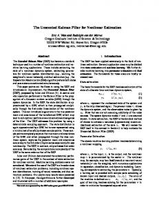
the Extended Kalman Filter (EKF). Using our experimental signals the performance of the EKF was not completely satisfactory. Sometimes estimation errors are too high and sometimes the filter may diverge. This is inappropriate for control loops [6]. Searching for a better alternative we selected the Unscented Kalman Filter (UKF) as a potentially better solution. While the EKF is based on the linearization of the model through Jacobians or Hessians, the UKF uses the non-linear model directly; therefore the predictions should be more accurate. The nine terms of the Direct Cosine Matrix (DCM) can be measured by using the Three Axis Attitude Determination (TRIAD) algorithm and data from on-board sensors: accelerometers and magnetometers. Using a quaternion formulation, which is a conventional way to deal with the attitude of aerial vehicles [7], the DCM terms can be easily handled. The quaternion approach is widely used in Attitude Heading Reference Systems (AHRSs) because it avoids the gimbal lock problem. With respect to numerical stability, quaternions are easier to propagate than the angles themselves. For systematic and non-risky work, a simulation environment has been developed. The core of the simulation is the X-Plane 9 simulator which is certified by the Federal Aviation Administration (FAA) for subsonic terrestrial flight. For realism, perturbations in the form of high-frequency noise and sensor latencies, are included to the data from the simulator. For evaluating the proposed solution, a number of simulations have been run. These have been used to both validate the solution and to compare it to the same algorithm using the EKF. During these simulations a maximum error of 1.0o is imposed on the pitch and roll attitude angles, and a maximum error of 4.0o on the yaw attitude angle. Under those requirements, which are standard in the industry [8], the error tolerances in the different signals are obtained through the analysis of a large number of simulation cases. The solution based on the UKF shows better performance. Finally, the UKF based solution is tested on a real experiment using a fixed-wing UAV of 2 meters of wingspan. This UAV is shown in figure 1. An in-house autopilot is used to test the estimation algorithm presented in this paper. The results of the solution are compared to different independent systems with very good results. Summarising, the first section of the paper presents some of the state of the art of AHRSs. The following section is devoted to the formulation of the problem, including the kinematic model and the TRIAD algorithm. Then comes a section describing the whole solution using the UKF and TRIAD. The

2

Fig. 1: UAV developed by the authors.

fifth section deals with data obtained by simulation, and the comparison between the UKF and the EKF is presented. Then, field experiments are presented to fully evaluate the proposed AHRS. In the final section of the paper, some conclusions are drawn, including some guidelines for future work. II. BACKGROUND AND RELATED WORK The Unscented Transformation (UT) and the UKF were introduced by Julier and Uhlmann [9], the algorithms were further explained, with examples, by Wan and Merwe [10]. An extensive description of the UKF was given in [11]. Background on the EKF algorithm is given in [12]. In [13] it was shown than the EKF can lead to unbounded estimation errors for nonlinear systems similar to those used in this paper. Some modern techniques, such as particle filters [14], are expensive in computational terms. Therefore they are unsuitable for microcontrollers unless the number of particles is reduced. However, this can lead to worse performance than the EKF [15]. In a recent article [16] a comparison of both the EKF and UKF is done for the particular case of flight path reconstruction for a fixed-wing UAV. This article includes an interesting discussion of previous references that illustrate the improved performance of the UKF over EKF estimating the attitude of an UAV. For real-time applications, it is important to reduce the computational cost. Part of the research deals with different ways of alleviating this cost. For instance, in [17] an attempt to simplify the observation model is shown; however, it compromises computational cost because the method involves the inversion of several large matrices every filter iteration. Another example is [18], which proposes to reduce the number of vector state variables. Our proposed solution has been implemented in a microcontroller for real-time estimation. As highlighted by [19] it is important to base the Kalman filter on an accurate model. In our context, the models presented in the following section are well established in the literature and correspond with experimental results. An extensive review of navigation systems is [20]. It covers different algorithms including Kalman filters and the TRIAD algorithm. The TRIAD algorithm was introduced by Shuster and Oh in [21] to measure the DCM in a spacecraft.

The use of IMUs based in MEMS technology to estimate the attitude angles in the industry has been increasing in the recent years, like a fastening tool tracking system in [22]. A well-known problem with gyrometers is bias. Therefore, different sensors have to be used to correct these biases. For instance, in [23] they are corrected using three-axis accelerometers. In [24] the use of eight accelerometers in a new configuration is proposed for measuring angular velocities in small UAVs. Different approaches rely on magnetometers [25], to be able to estimate yaw angle in helicopters, or in GPS [26] to estimate the position as well the attitude in fixedwing UAVs. Alternatively, other papers propose not to use gyrometers at all in conventional aircrafts, but several GPS receivers instead [27]. In this paper we propose an attitude estimator using the UKF and the TRIAD algorithm involving gyrometers, magnetometers and accelerometers. The validation of the algorithm is done by both simulations and field experiments. Experiments use an on-board hardware with MEMS sensors. III. P ROBLEM FORMULATION Although each UAV has its own coefficients and therefore its own dynamical model, it is possible to determine Euler angles from a kinematic model, which is independent of the UAV’s coefficients. In this section we derive the mathematical formulation of the AHRS problem in a UAV equipped with a three-axis gyrometer, three-axis accelerometer and three-axis magnetometer. A. AHRS kinematic model The Euler angles describe the aircraft body-axis orientation in north, east, and down coordinates. That means in longitudinal, lateral and normal coordinates, with respect to the local tangent plane to the Earth and true north. Here θ is the pitch angle, φ the roll angle and ψ is the yaw angle according to Figure 2. The angular velocity vector expressed in body frame is P for the roll rate, Q is the pitch rate and R is the yaw rate; and it is related to the Earth frame by the transformation given by the kinematics equation (1).    ˙  1 tan θ sin φ tan θ cos φ φ P  θ˙  = 0 cos φ − sin φ  Q (1) cos φ sin φ R 0 ψ˙ cos θ cos θ Integrating equation (1) gives numerical instability and could be gimbal locked. For this reason, a quaternion formulation to represent the attitude is preferred: 3 P

q = q0 + q1 i + q2 j + q3 k

qi = 1

(2)

i=0

Where the quaternion norm is 1 and their components from Euler angles are: q0 = cos φ0 cos θ0 cos ψ 0 + sin φ0 sin θ0 sin ψ 0

(3)

0

0

0

0

0

0

(4)

0

0

0

0

0

0

(5)

q3 = cos φ0 cos θ0 sin ψ 0 − sin φ0 sin θ0 cos ψ 0

(6)

q1 = sin φ cos θ cos ψ − cos φ sin θ sin ψ q2 = cos φ sin θ cos ψ + sin φ cos θ sin ψ

3

Another issue arises when the equation (7) is integrated. The quaternion shall conserve its norm equals to 1, otherwise the Euler angles are wrongly computed from the quaternion. Although it can be normalized after every integration step, there is a better way to do it. The quaternion norm can be kept solving the equation (7) using the next integrating factor:   t Z (14) exp  Ω d t t0

where 

Fig. 2: Axes and coordinate definitions. where φ0 = φ/2, θ0 = θ/2, and ψ 0 = ψ/2. The kinematics equation (1) can be rewritten in linear form using quaternion components:      0 −P −Q −R q0 q˙0  q1  q˙1  1 P 0 R −Q    =  (7) q˙2  2 Q −R 0 P  q2  R Q −P 0 q3 q˙3 Additionally, it is useful to formulate the DCM using quaternion components and the Euler angles from the DCM terms: DCM ≡ A = {cij } =   A1 2(q1 q2 + q0 q3 ) 2(q1 q3 − q0 q2 ) 2(q1 q2 − q0 q3 ) A2 2(q2 q3 + q0 q1 ) 2(q1 q3 + q0 q2 ) 2(q2 q3 − q0 q1 ) A3

(8)

where A1 = q02 + q12 − q22 − q32 , A2 = q02 − q12 + q22 − q32 , and A3 = q02 − q12 − q22 + q32 . Then, θ = − arcsin(2(q1 q3 − q0 q2 )) φ = atan2(2(q2 q3 + ψ = atan2(2(q1 q2 +

q0 q1 ), q02 q0 q3 ), q02

(9) − +

q12 q12

− −

q22 q22

+ −

q32 ) q32 )

(10) (11)

0 −P 1 P 0 Ω=  2 Q −R R Q

Denoting the angular velocity vector ω = (P, Q, R), if the gyros from the sensors are ωs , they can be corrected using the bias as: ω = ωs − b

(13)

(15)

Assuming that the angular velocities remain constant during the interval d t, we can discretize the equation (7) as follows [29]: k∆ωk k∆ωk + sin k∆ωkΩ q(k) (16) q(k + 1) = I cos 2 2 p where k∆ωk = 12 (P ∆t)2 + (Q∆t)2 + (R∆t)2 and I is the identity matrix. C. The TRIAD algorithm The Three Axis Attitude Determination algorithm was introduced by Shuster and Oh [21] to determine the attitude in a Spacecraft from a set of vector measurements. TRIAD is a deterministic method to compute the DCM. Given the reference unit vectors V1 and V2 and the corresponding observation unit vectors W1 and W2 , the DCM satisfies: AV1 = W1

AV2 = W2

(17)

The TRIAD algorithm determines the DCM using the following expression

where atan2 is the four-quadrant version of the inverse tangent function, and arcsin is the arcsine function. B. Gyros integration problem The three-axis gyrometer measures the angular velocities, and for obtaining the Euler angles, the gyros can be integrated using equation (7). However, even if we ignore the sensor noise, the gyros usually have bias, making integration their error grow in every step. Fortunately for a MEMS gyrometer in normal conditions (not extremal temperature or pressure variation), this bias can be assumed to be constant [28], or very slow varying throughout the UAV mission. Therefore the bias for the gyrometer can be modeled as: T b˙ = 0 with b = bx by bz (12)

 −Q −R R −Q  0 P  −P 0

A = Mo MrT

(18)

Mo = (o1 |o2 |o3 )

(19)

Mr = (r1 |r2 |r3 )

(20)

where the observation column vectors oi and the reference column vectors ri are given by o1 = W1

(21)

o2 = (W1 × W2 ) /|W1 × W2 |

(22)

o3 = (W1 × (W1 × W2 )) /|W1 × W2 |

(23)

r1 = V1

(24)

r2 = (V1 × V2 ) /|V1 × V2 |

(25)

r3 = (V1 × (V1 × V2 )) /|V1 × V2 |

(26)

Notice that the pair (W1 , V1 ) has more influence on A than (W2 , V2 ), this is because part of the information contained in the second pair is discarded. Therefore it is convenient to assign (W1 , V1 ) to the pair of greater accuracy, which depends on the flight circumstances. Section IV-B describes criteria to assign these pairs.

4

IV. U NSCENTED K ALMAN F ILTER DESIGN The UKF [9] is an alternative to the EKF, providing superior performance at similar order of computational cost. Also during the UKF implementation process, there are not Jacobians, Hessians or other derivatives involved. In this paper, the UKF is used both for state estimation (quaternion components) and for parameter estimation (gyrometer’s biases). The estimation algorithm is implemented as a two-step propagator/corrector filter. It is desirable to run each step as many times as possible, however, the frequencies at which they will be run will be limited by different factors. For the propagation step, the limiting factor is the computation time; we chose a frequency of 100 Hz. The correction step is limited, in our case, by the GPS sample rate, that is, 1 Hz. The algorithm is described in the diagram shown in Figure 3. The diagram depicts the two main loops, one at 100 Hz and the other at 1 Hz, these loops correspond to the propagation and correction steps respectively. It can be noted how the TRIAD information feeds the correction step. ,-.'.%/ 0#-1.'.#-) ?!@ 8%':8#-:=/' 23345 !*+

245

!"#$%&%'( )'%'(

% 6 7

8#9:$%)) ;./'("

E#"7%/.5( )(-)#" A%/F()

x ˆ0 = E[x0 ] P0 = E[(x0 − x ˆ0 )(x0 − x ˆ0 ) ]

(29)

At the start of every iteration we calculate the sigma points [9] χk−1 of the quaternion components and gyro’s biases. p p χk−1 = x ˆk−1 − γ Pk−1 (30) ˆk−1 x ˆk−1 + γ Pk−1 x √ Where γ = L + λ, λ is a composite √ scaling parameter and L is the state vector dimension. Pk can be computed with the lower triangular Cholesky factorization. The next step is to evaluate the model on the sigma points: χ∗k|k−1 = F [χk−1 , uk−1 ]

Where F is the process model as given by equations (16) and (12). uk−1 is the angular velocity vector ω. The a priori state estimation is approximated using a weighted sample mean

B#"/1 C%&-('.D C#1(/

x ˆ− k = Fig. 3: Algorithm block diagram. !

(28) T

0#""(D' )'%'(

?!@:A(/ 6

Where qi are the quaternion components and bj are the gyrometers’ biases. These are assumed to be Gaussian Random Variables (GRVs). Their process model is given by equations (16) and (12), respectively. The basis of the UKF is the UT; which is a method for calculating the statistics of a random variable which undergoes a nonlinear transformation [9]. In our case, we assume that the noise of the UAV sensors is additive (zero mean). Under this assumption, the equations to estimate the Euler angles and the gyrometer’s biases are the ones described in this subsection. The computation algorithm begins with the initial conditions:

2L X

(m) ∗ χi,k|k−1

Wi

(31)

(32)

i=0

!

where The area surrounded by dashed lines contains the elements involved in the TRIAD calculations. The leftmost block represents an access to the sensors to measure b a and b m which correspond to the accelerations and magnetic field measurements in the body reference frame respectively. The signals are then filtered. The GPS velocity is used to subtract the centrifugal accelerations as explained in subsection B; which also covers the description of the TRIAD block. On the right side of the diagram the block denoted as World Magnetic Model uses an harmonic spherical model to obtain the magnetic field vector at the position of the UAV. This vector is used as one of the references in the TRIAD algorithm. This section describes the design of the filter under the considerations given above. Subsection A gives the equations involved in the propagation loop whilst Subsection B deals with those of the correction loop.

(m)

W0

= λ/(L + λ)

(33)

(m) Wi

= 1/ (2(L + λ))

(34)

and the covariance matrix is Pk− =

2L X

(c)

∗ T Wi [χ∗i,k|k−1 − x ˆ− ˆ− k ][χi,k|k−1 − x k ] + Qnoise

i=0

(35) where (c)

W0

= λ/(L + λ) + (1 − α2 + β)

(36)

(c) Wi

= 1/ (2(L + λ))

(37)

The constant α determines the spread of the sigma points around x ˆ and is usually set to a small positive value (for instance, 1 ≤ α ≤ 1e−4 ). The constant β can be used to incorporate prior knowledge of the distribution of the state A. Propagation equations and process model Gaussian distributions, β = 2 is optimal [10]. This subsection describes the propagation loop. The state vector: for 7x7 Q ∈ R is the process noise covariance: noise vector is: T Qq 0 x(k) = q0 (k) q1 (k) q2 (k) q3 (k) bx (k) by (k) bz (k) Qnoise = (38) 0 Qb (27)

5

where Qq ∈ R4x4 is the noise covariance associated to the quaternion components and Qb ∈ R3x3 is the noise covariance associated to the gyrometer biases. The process that relates the quaternion components and angular velocities has a continuous-time analytical solution, as was shown in Subsection III-B. However, the discretetime equation (16) assumes that the angular velocities remain constant during the discretization period. Hence, Qq should be close, but different to zero. For the simulation and experimental results shown in this paper: Qq = 1 × 10−6 · I4x4

(39)

where I4x4 is the 4x4 identity matrix. The process noise covariance associated to the gyrometer biases Qb is the 3x3 zero matrix. The rationale for this is the same that explains equation (12) in Subsection III-B. B. Correction equations and observation model Even though the TRIAD algorithm gives the nine terms of the DCM (see equation (8)), only four of them are needed to calculate the Euler angles. Hence, the observation function has been designed to measure these four terms. To determine the pitch and roll angles, the terms are the X and Y components of the Z earth vector expressed in the body frame. b

ZEx ≡ c13 = 2(q1 q3 − q0 q2 )

(40)

b

ZEy ≡ c23 = 2(q2 q3 + q0 q1 )

(41)

For the yaw angle, the terms are the X and Y components of the X body vector expressed in the Earth reference frame. E

Xbx ≡ c11 = (q02 + q12 − q22 − q32 )

(42)

E

Xby ≡ c12 = 2(q1 q2 + q0 q3 )

(43)

Therefore, the observation model is given by equation (44). T H(xk ) = c13 c23 c11 c12 (44) According to the TRIAD algorithm two vector pairs are needed to compute the terms of the DCM. Each pair consists of a measure or observation and a reference vector (equation (17)). In our case, these pairs are the magnetic field, and the acceleration of the UAV. The magnetic observation vector is the field measured at body frame. The magnetic reference vector is the Earth’s magnetic field using an harmonic spherical model; the geographical coordinates for this model are provided by an onboard GPS receiver. For the acceleration pair, the observation is given by the on-board IMU. It should be noted that the measurement given by the accelerometers includes: linear acceleration, Coriolis acceleration, centripetal acceleration and gravity. Coriolis acceleration is assumed to be negligible, in our experiments −4 it is of the order of 10 g. The reference is the Earth’s ˆ = 0 0 1 , normalized in North East Down gravity g (NED) coordinates. The on-board accelerometers are affected by mechanical vibrations and environmental perturbations, therefore it is convenient to use a low-pass filter to reduce these

effects. Also, the centrifugal contribution of the acceleration has to be subtracted: aN = U˙ + QW − RV (45) E ˙ aE = V + RU − P W (46) E ˙ + P V − RU aD = W (47) Where the speed b V = U V W is expressed in the body frame of reference. In a fixed-wing UAV, during a nonacrobatic flight, both V and W are negligible. Therefore, the GPS speed measurement gives U , which is the dominant component of b V. As stated in section III-C it is convenient to assign (W1 , V1 ) to the pair of greater accuracy. During a flight, there are times when accelerometers offer more accuracy, whereas during others, magnetometers are more reliable. In our case, we used the following criteria. In order of priority: • If 0.9ˆ g ≤ |b a| ≤ 1.1ˆ g then it can be assumed that this is a stationary flight, hence the acceleration is the pair of ˆ and W1 = b a. greater accuracy. In this case, V1 = g b • Else, if 0.7ˆ g < | a| < 0.9ˆ g or 1.1ˆ g < |b a| < 1.3ˆ g then it can be assumed that the plane is doing a coordinated turn. In this case, magnetometers offer greater accuracy. Therefore, V1 = E m and W1 = b m. b E b E • Else, if | m| > 1.2| m| or | m| < 0.8| m| then the magnetic measurements are not reliable. The correction step is skipped. b • Else, if | a| > 1.3ˆ g or |b a| < 0.7ˆ g then it is assumed that the current state is acrobatic and neither the magnetic measurements nor the acceleration measurements are reliable enough. The correction step is skipped. ˆ the Where E m is the Earth’s magnetic field vector and g Earth’s gravity acceleration. Notice how in the last two cases, the correction step is skipped. The following only applies in the first two cases. The UKF begins the correction step by redrawing the sigma points. This is done to incorporate the effect of the additive noise [10]. h q i q (48) χk|k−1 = x Pk− x ˆ− Pk− ˆ− x ˆ− k −γ k k +γ E

Then the unscented transformation of the observations is computed. Yk|k−1 = H[χk|k−1 ] yˆk− =

2L X

(m)

Wi

Yi,k|k−1

(49) (50)

i=0

The measure and cross-covariance matrices are Py¯k y¯k =

2L X

(c)

Wi [Yi,k|k−1 − yˆk− ][Yi,k|k−1 − yˆk− ]T + Rnoise

i=0

(51) Pxk yk =

2L X

(c)

Wi [χi,k|k−1 − x ˆ− ˆk− ]T k ][Yi,k|k−1 − y

(52)

i=0

where Rnoise is the measurement noise covariance. The value of Rnoise can be derived from the nominal values of the errors of

6

the sensors involved. This derivation is described thoroughly in [21]. Now the Kalman gain is computed:

Roll rate True value Corrupted value 2

Kk = Pxk yk Px−1 k yk x ˆk = x ˆ− ˆk− ) k + Kk (yk − y Pk =

Pk−

−

Kk Py¯k y¯k KkT

(53) (54)

Degrees / sec

1.5

Finally, the correction equations are (53) and (54):

1

0.5

V. S IMULATIONS RESULTS Since real experiments might imply crashes, some previous simulations are in order. For this, we developed a simulation framework, which consists in three different parts. The core of the simulation is the X-Plane 9 software. The other two parts are: the plug-in code for X-Plane 9 and the model of the sensors. The idea is to integrate a six-degree-of-freedom aerodynamic model, provided by X-Plane with a realistic model of the sensors we are using. The plug-in code is just the glue between them. X-Plane 9 includes different aircraft models. Its default radio control model is very similar to our UAV, so no modifications to it are needed. This is the model used in the simulations of this section. The purpose of the simulations is to study the effects of sensor noise, bias and latencies. Therefore, the model of the sensors focuses on these aspects: • GPS signal is delayed 1 second. • Gyrometers signal are biased and corrupted with white noise. • Accelerometers are biased and corrupted with colored noise, focusing in high frequencies. • Magnetometers are biased and corrupted with white noise. Figure 4 shows an example of how bias and noise are added to a variable. Notice how both the magnitude of the noise and the bias are kept constant throughout the simulation. In particular, the example shows roll rate measurements as simulated. A first target of the simulations is to study the tolerances of both estimators to bias and noise magnitude. According to standard procedures, a maximum error of 1.0o in the estimation of pitch and roll angle, and 4.0o for yaw angle are imposed. It is assumed that with this error it is possible to do closed-loop control. This is covered in the first part of this section. The second part of this section assesses the performance of the UKF using real values for the biases and noise magnitudes of our sensors.

0

376.5

376.6

376.7

376.8 Time (s)

376.9

377

377.1

Fig. 4: True and corrupted roll rate used for simulations. TABLE I: UKF tolerances: Maximum bias and random error standard deviation. Measurement

Bias error

Random error

Roll rate, P Pitch rate, Q Yaw rate, R Accelerometers Magnetometers GPS Velocity

±9.98 o /sec ±9.98 o /sec ±9.98 o /sec ±0.3 m/s2 ±10.53mG ±2.57m/s


It can be noted how both algorithms are more sensitive to errors in R than they are to errors in P and Q. This is because the information in the yaw angle is only provided by one of the sensors, the magnetometer. While the information in pitch and roll angles are provided by the accelerometer and the magnetometer. In general, EKF is more sensitive to biases and noises than the UKF. In particular it is very sensitive to the bias in R. Hence, the solution based on the UKF is preferred. B. Simulation using real error values For this simulation, the real biases and noise magnitudes were extracted from our IMU’s datasheet. Table III shows them. It is interesting to compare these values to those from tables I and II. It can be seen how some errors are outside of the EKF tolerances. So EKF can not be used in our case. TABLE II: EKF tolerances: Maximum bias and random error standard deviation.

A. Error tolerances and comparison of estimators A Monte Carlo analysis of the tolerances was made, supported by a batch of simulation experiments. Each of the experiments specifies different values of biases and noise magnitudes, which were drawn from a Gaussian distribution. Two sets of results were obtained, one using the UKF and the other using the EKF. These sets are shown in Tables I and II respectively.

Measurement

Bias error

Random error




7

TABLE III: Typical MEMS bias and random error standard deviation. Bias error

Random error




estimated value true value

4

2

Degrees

Measurement

Pitch 6

0

−2

4

3

2

1 −4

Figures 5, 6 and 7 show the behavior of the UKF algorithm in a typical flight in a windy scenario. Solid lines depict simulated angles while the dashed ones depict estimations from the AHRS. It should be noted that in figure 7, the abrupt changes near seconds 520 and 590 is due to the representation of angles in the range ±180o . The agreement between the simulated and estimated values is satisfactory.

−6 RMSE 0.4776 deg 350

400

450

500 Time (s)

550

600

Fig. 6: Pitch angle simulated with MEMS parameters. Yaw estimated value

Roll

true value

100

10

50 Degrees

4

3

2

1 Degrees

true value

150

estimated value 15

5

0

−50

−5

−100

4

3

2

1

0

−150

−10

RMSE 1.1529 deg

RMSE 0.5481 deg −15 350

350

400

450

500 Time (s)

550

600

Fig. 5: Roll angle simulated with MEMS parameters. Area marked with ’1’ shows a coordinated turn to the left, note how the yaw angle decreases. This turn leads to the next area, marked with ’2’, which is a steady flight. The area marked with ’3’ is a new coordinated turn to the right, note how the yaw angle increases. The final area, marked with ’4’, is a new steady flight; the three angles remain mostly constant. It can be noted that the pitch angle estimation in area ’4’ has a slight bias (of less than 0.3o ), this is due to the magnetometers biases added during the data corruption. These biases are not compensated through the algorithm because of their negligible effect compared to the gyrometers biases. The pitch and roll angles experience vibrations due to different gusts of wind. This section has shown how the simulation results give confidence on the AHRS using the UKF. The system can be used in field experiments. The following section covers field experiments and the validation of the AHRS. VI. F IELD EXPERIMENT RESULTS The target of the research is to use the AHRS to feed a closed-loop controller in field experiments. Aside from the

400

450

500 Time (s)

550

600

Fig. 7: Yaw angle simulated with MEMS parameters.

simulation results presented in an earlier section, an experimental validation of the system has been done. Experiments were carried out using a small fixed-wing UAV. An on-board autopilot hardware has been designed and built for this UAV. Figure 8 shows a functional diagram of the autopilot. Two ARM7 microcontrollers are used for sensor data handling and navigation algorithms. Both are connected with a UART channel. Flight data are measured by different sensors: a GPS receiver, an IMU with magnetometers, and four pressure sensors. One of the pressure sensors is used as a barometer for altitude measurement and the rest, one per axis, are connected to Pitot tubes for air-speed measurement. Sensor data are stored in an SD card for experiment analysis. The IMU used is the ADIS16405 from Analog Devices. The navigation microcontroller receives processed sensor data from the other microcontroller, and sends this data over the radio link. In future, when the control loop is closed, this microcontroller will send the PWM signals to the actuators. Figure 9 shows a picture of the autopilot.

8

Fig. 8: Functional diagram of the autopilot.

Fig. 10: One of the frames processed by the vision system.

angle and the measurements from the vision system. The area marked with ’1’ depicts the end of a turn to the right. Is is followed by a steady flight in the area marked with ’2’, finally leading to another turn to the right in the area marked with ’3’. The results of the comparison are clearly satisfactory. Vision vs UKF roll angle 30

Vision range UKF estimation

1

3

25

Degrees

20

Fig. 9: Photograph of the on-board hardware next to the UAV.

15

2 10 5 0

The target of the experiments is to assess the accuracy of the estimation of each of the three attitude angles. Therefore, experiments are designed to excite the single modes of the system, that is, pure roll, pure pitch and pure yaw. However, due to the nature of the system, it is not possible to do so in practice; there is always some coupling between motions. We tried to excite these modes during the experiments. In addition, typical maneuvers such as coordinated turns were also included. A ground station was built to receive data from the UAV using a radio link. The flight is manually controlled using a conventional radio control unit. For validation purposes, data coming from independent sensors (not used by the estimation algorithm) have been considered. For the roll angle, a computer vision system is used. The GPS velocity is used to validate the yaw angle. The vision system uses a small camera attached to the UAV. An algorithm was developed to obtain the roll angle from the video measuring the slope of the horizon. The algorithm is based on [30] [31] [32]. Figure 10 shows one of the frames taken during the flight and processed by the vision system. The results of this system have an uncertainty of ±3o . Figure 11 shows a comparison between the estimated roll

−5 2

4

6

8 Time (s)

10

12

14

Fig. 11: Roll angle comparison between vision system and UKF estimation. The actual experiment took place under adverse atmospheric conditions, in particular, there were gusts of wind. So when there is strong crosswind, the yaw angle differs from the heading of the plane. The heading is measured using the GPS velocity with an uncertainty of ±10o . It can be noted that the GPS velocity is only used to subtract the centrifugal contribution of the accelerometers (see equation (47)) in the estimation algorithm. Therefore, it can be taken as an independent system for validation purposes. Figure 12 shows a comparison of the estimation of the yaw angle and the heading measured by the GPS. The figure corresponds to a turn of 360o . During the area marked with ’1’, the UAV faces the wind gusts. The area marked with ’2’ shows the effect of crosswind; it makes the yaw angle and the heading diverge. In other words, the UAV does not move in

9

the direction it points to. Finally, throughout the area marked with ’3’, the UAV has tail wind and the yaw angle closely follows the GPS heading. Yaw 200

2

1

3

150 100

Degrees

50 0

The performance of the algorithm has been assessed using field experiments. Using independent sensors it has been checked that the estimation algorithm gives good results. A possible idea for future research is to include the information from these sensors into the AHRS itself. Since the estimation results are encouraging the next experimental work will be to feed the estimations to a closed-loop controller. Due to space constraints only some snapshots of the experimental results have been shown. However, the complete set of data confirm the good quality of the estimations. This gives confidence on the algorithm, which is easy to implement and it can be run on an on-board microcontroller.

−50

R EFERENCES −100

GPS range UKF estimation

−150 −200

0

5

10

15

20 25 Time (s)

30

35

40

45

Fig. 12: Yaw angle comparison between GPS system and UKF estimation. With the sensors we are currently using, it is not possible to have an independent measurement of the pitch angle. However, due to the formulation of the algorithm using quaternions, the pitch angle is strongly coupled to the roll and yaw angles. Therefore, it can be assumed that if both the roll and yaw angles are correctly estimated, the pitch angle is correctly estimated too. VII. C ONCLUSIONS . This paper considered the problem of attitude estimation of an UAV in order to establish closed-loop control. The mathematical formulation of the problem has been presented in terms of quaternions. The on-board AHRS is based on a MEMS IMU. A widely used estimator is the Kalman Filter. The kinematic model of aircraft attitude is highly non-linear, so a version of the Kalman filter able to cope with non-linearities is needed. Two of these versions, have been studied: the EKF and the UKF. A common solution in the satellite attitude estimation practice is the TRIAD algorithm and it has been used as the observation model in the UKF framework in this paper. Previous studies in the attitude determination field give the same confidence to the sensors throughout the whole UAV mission. This is unsuitable for missions that mix both acrobatic and non-acrobatic maneuvers. Using the TRIAD algorithm it is easy to select the most reliable sensors along the different phases of a flight. Criteria for this selection have been described. A simulation framework based on XPlane 9 has been introduced. This simulation corresponds to the characteristics of the experimental UAV. Using simulation results, it was found that the UKF shows better performance than the EKF. Therefore, the UKF has been used in the final version of the AHRS.

[1] I. Maza, F. Caballero, J. Capitan, J. M. de Dios, and A. Ollero, “Firemen monitoring with multiple uavs for search and rescue missions,” in Proc. IEEE Workshop on Security, Safety and Rescue Robotics (SSRR), 2010. [2] D. T. Cole, S. Sukkaireh, and A. H. Göktogan, “System development and demonstration of a uav control architecture for information gathering missions,” Journal of Field Robotics, no. 26, pp. 417–440, 2006. [3] Y. Xia, Z. Zhu, M. Fu, and S. Wang, “Attitude tracking of rigid spacecraft with bounded disturbances,” IEEE Transactions on Industrial Electronics, vol. 58, no. 2, pp. 647–659, 2011. [4] B. Zheng and Y. Zhong, “Robust attitude regulation of a 3-dof helicopter benchmark: Theory and experiments,” IEEE Transactions on Industrial Electronics, vol. 58, no. 2, pp. 660–670, 2011. [5] Z. Zhu, Y. Xia, and M. Fu, “Adaptive sliding mode control for attitude stabilization with actuator saturation,” IEEE Transactions on Industrial Electronics, vol. PP, 2011. [6] G. Cai, B. Chen, K. Peng, M. Dong, and T. Lee, “Modeling and control of the yaw channel of a uav helicopter,” IEEE Transactions on Industrial Electronics, vol. 55, no. 9, pp. 3426–3434, 2008. ˇ [7] O. Spinka, O. Holub, and Z. Hanzálek, “Low-cost reconfigurable control system for small uavs,” IEEE Transactions on Industrial Electronics, vol. 58, no. 3, pp. 880–889, 2011. [8] L. B. Stephen A. Whitmore, Mike Fife, “Development of a closed-loop strap down attitude system for an ultrahigh altitude flight experiment,” NASA Technical Memorandum 4775, 1997. [9] S. J. Julier and J. K. Uhlmann, “A new extension of the kalman filter to nonlinear systems,” in Proc. Int. Symp. Aerospace/Defense Sensing, Simul. and Controls, Orlando, FL, 1997, pp. 182–193. [10] E. Wan and R. van der Merwe, “The unscencted kalman filter,” in Kalman Filtering and Neural Networks, S. Haykin, Ed. Wiley, 2001, ch. 7. [11] S. J. Julier and J. K. Uhlmann, “Unscented filtering and nonlinear estimation,” in Proceedings of the IEEE, vol. 92, no. 3, 2004, pp. 401– 422. [12] A. H. Jazwinski, Stochastic Processes and Filtering Theory. Academic Press, Inc., 1970. [13] K. Reif, S. Gunther, E. Yaz, and R. Unbehauen, “Stochastic stability of the discrete-time extended kalman filter,” IEEE Transactions on Automatic Control, vol. 44, no. 4, pp. 714–728, April 1999. [14] F. Gustafsson, F. Gunnarsson, N. Bergman, U. Forssell, J. Jansson, R. Karlsson, and P.-J. Nordlund, “Particle filters for positioning, navigation, and tracking,” IEEE Transactions on Signal Processing, vol. 50, no. 2, pp. 425–437, Feb. 2002. [15] S. P. Won, W. W. Melek, and F. Golnaraghi, “A kalman/particle filterbased position and orientation estimation method using a position sensor/inertial measurement unit hybrid system,” IEEE Transactions on Industrial Electronics, vol. 57, no. 5, pp. 1787–1798, May 2010. [16] B. O. Teixeira, L. A. Tôrres, P. Iscold, and L. A. Aguirre, “Flight path reconstruction - a comparison of nonlinear kalman filter and smoother algorithms,” Aerospace Science and Technology, vol. In Press, Corrected Proof, 2010. [17] J. Marins, X. Yun, E. Bachmann, R. McGhee, and M. Zyda, “An extended kalman filter for quaternion-based orientation estimation using marg sensors,” in Proc. IEEE/RSJ International Conference on Intelligent Robots and Systems., vol. 4, 2001, pp. 2003–2011. [18] M. J. Hale, P. Vergez, M. J. Meerman, and Y. Hashida, “Kalman filtering and the attitude determination and control task,” in Proc. AIAA Space Conference and Exhibit, Sept. 2004, paper AIAA-2004-6018.

10

[19] J. Qi, J. Han, and Z. Wu, “Rotorcraft uav actuator failure estimation with kf-based adaptive ukf algorithm,” in American Control Conference, June 2008, pp. 1618–1623. [20] A. M. Hasan, K. Samsudin, A. R. Ramli, R. S. Azmir, and S. A. Ismaeel, “A review of navigation systems (integration and algorithms),” Australian Journal of Basic and Applied Sciences, vol. 3, no. 2, pp. 943–959, 2009. [21] M. D. Shuster and S. D. Oh, “Three axis attitude determination from vector observations,” Journal of Guidance and Control, vol. 4, no. 1, pp. 70–77, Jan. 1981. [22] S. P. Won, F. Golnaraghi, and W. W. Melek, “A fastening tool tracking system using an imu and a position sensor with kalman filters and a fuzzy expert system,” IEEE Transactions on Industrial Electronics, vol. 56, no. 5, pp. 1782–1792, May 2009. [23] D. Du, L. Liu, and X. Du, “A low-cost attitude estimation system for uav application,” in Chinese Control and Decision Conference (CCDC), May 2010, pp. 4489–4492. [24] S. Lei, H. Chang-qiang, W. Xing-wei, and W. Wen-chao, “Research on a new eight-accelerometer configuration for attitude angle calculation of uav,” in Chinese Control and Decision Conference (CCDC), May 2010, pp. 4119–4123. [25] W. YongLiang, W. TianMiao, L. JianHong, W. ChaoLei, and Z. Chen, “Attitude estimation for small helicopter using extended kalman filter,” in IEEE Conference on Robotics, Automation and Mechatronics, Sept. 2008, pp. 577–581. [26] J. S. Jang and D. Liccardo, “Small uav automation using mems,” IEEE Aerosp. Electron. Syst. Mag, vol. 22, no. 5, pp. 30–34, May 2007. [27] D. Gebre-Egziabher, G. Elkaim, J. Powell, and B. Parkinson, “A gyro-free quaternion-based attitude determination system suitable for implementation using low cost sensors,” in IEEE Position Location and Navigation Symposium, 2000, pp. 185–192. [28] A. E. Hadri and A. Benallegue, “Sliding mode observer to estimate both the attitude and the gyro-bias by using low-cost sensors,” in IEEE/RSJ International Conference on Intelligent Robots and Systems (IROS), Oct. 2009, pp. 2867–2872. [29] J. Vaganay, M. Aldon, and A. Fournier, “Mobile robot attitude estimation by fusion of inertial data,” in Proc. IEEE International Conference on Robotics and Automation, vol. 1, May 1993, pp. 277–282. [30] J.-C. Bazin, I. Kweon, C. Demonceaux, and P. Vasseur, “Uav attitude estimation by vanishing points in catadioptric images,” in IEEE International Conference on Robotics and Automation (ICRA), May 2008, pp. 2743–2749. [31] H.-Z. Yuan, X.-Q. Zhang, and Z.-L. Feng, “Horizon detection in foggy aerial image,” in International Conference on Image Analysis and Signal Processing (IASP), Apr. 2010, pp. 191–194. [32] G. Pereira, P. Iscold, and L. Torres, “Airplane attitude estimation using computer vision: simple method and actual experiments,” Electronics Letters, vol. 44, no. 22, pp. 1303–1304, Oct. 2008.