Open Access Library Journal
Anchoring Heuristic Messes with Inflation Targeting Evelin Da Silva1, Sergio Da Silva2* 1
Department of Economics and International Relations, Federal University of Santa Catarina, Florianopolis, Brazil 2 Graduate Program in Economics, Federal University of Santa Catarina, Florianopolis, Brazil Email: *
[email protected] Received 25 March 2015; accepted 9 April 2015; published 14 April 2015 Copyright © 2015 by authors and OALib. This work is licensed under the Creative Commons Attribution International License (CC BY). http://creativecommons.org/licenses/by/4.0/
Abstract We evaluate recent inflation-targeting using Brazilian data and also consider the framework of the macroeconomic model of adaptive learning blended with a cognitive psychology approach. We suggest that forecasters interpret the inflation target as an anchor, and adjust to it accordingly. As current inflation increases above the target level, a central bank loses credibility, and forecasters start the adjustment from the top because they expect an even higher future inflation. Then, they move back to the core target within a range of uncertainty, but the adjustment is likely to end before the core is reached, as predicted by the psychological theory of anchors. After calibrating the model, we find an asymptotic equilibrium of a 6.1 percent inflation rate, which overshoots the announced target inflation core of 4.5 percent. This example casts doubt on the very justification for inflation targeting, which is unlikely to succeed when private forecasters rely on anchoring heuristics.
Keywords Anchoring Heuristic, Inflation Targeting, Adaptive Learning Subject Areas: Behavioral Economics
1. Introduction In the last 20 years, many academic macroeconomists [1] [2] and policymakers worldwide have been favoring the adoption of a monetary policy framework called “inflation targeting.” Its alleged advantages are lower, less variable inflation and interest rates, and more stable economic growth. This harmonious environment could be attainable because of an enhanced ability of central banks to respond credibly to the random shocks hitting *
Corresponding author.
How to cite this paper: Da Silva, E. and Da Silva, S. (2015) Anchoring Heuristic Messes with Inflation Targeting. Open Access Library Journal, 2: e1450. http://dx.doi.org/10.4236/oalib.1101450
E. Da Silva, S. Da Silva
economies. It has to be said, however, that this standpoint remains popular despite the fact that evidence on the effectiveness of inflation targeting is mixed. One key study [3] showed that, when compared with economies that did not adopt inflation targeting, its use by a group of developed economies could not be credited to bringing down inflation and inflation volatility. For “emerging” economies, adoption of inflation targeting did not receive empirical support for boosting economic growth [2]. Our study adds to skeptical literature: We take Brazilian data and find that its inflation targeting is unlikely to succeed when private forecasters rely on anchoring heuristics. This result was evident after we adopted a new cognitive psychology perspective in connection with the traditional macroeconomic approach of bounded rationality with adaptive learning in the inflation forecasts.
2. Materials and Methods We collected raw inflation data based on monthly series of the Brazilian broad price index (called IPCA) from November 2001 to September 2013. We considered datapoints of monthly frequency, and used the last day of the month as representative of a month. An alternative date could be the day after the release of the so-called IPCA-15 (an index strongly correlated with the IPCA; correlation = 0.986). We choose the last day of the month because forecasters are already in possession on that date of the information of the previous month’s inflation. The data on inflation forecasts made by professional forecasters (called “market expectation system”) are considered by the Brazilian central bank for the following 12 months (“the long run”). We took the inflation expectation data from such a central bank source and considered, as usual, the median of the time interval from November 2001 to September 2013. The median value was used in our analysis for calibrating the forecasters’ predictions 12 months forthcoming, from October 2002 to August 2014. The median is taken to prevent possible distortions in forecasts collected on a daily basis. The median is also justified because the central bank can lose credibility in the meantime, in which case private forecasters tend not to reveal their true expectations. All the data employed in this work are available at http://dx.doi.org/10.6084/m9.figshare.1310598. Competition between the professional forecasters is promoted by the Brazilian central bank, which rewards the year’s top five forecasters. This aims to improve the quality of data collected from the market expectation system. As a result of this incentive mechanism, we considered the source of data rather than the alternative of gauging the inflation expectations embodied in the prices of assets. However, the central bank data themselves are far from perfect. Table 1 shows the top five private forecasters for 2009 to 2013. Any conclusions from Table 1 will fall victim to the “law of small numbers,” because the data are collected for only five years. However, if the pattern in Table 1 continues as more and more years are added in the future, one can infer the central bank is rewarding luck rather than forecasting talent. Indeed, there is no consistent winner among those in the top five each year. Apparently, no central bank officer seems to have compared the annual data as we did in Table 1, which is strongly suggestive of “regression to the mean” at work: A high-performance forecaster one year becomes a poor forecaster in the next. Table 1 also reveals mean regression for the annual sets of forecast errors. Groups of forecasters seem to make similar predictions, which result in either high or low aggregate sets of forecast errors. The consequence is an annual cycle for their errors: In 2009 the errors were low, but they went up the next year (2010). The errors dropped in 2011, and they increased in 2012, only to drop again in 2013. Interestingly, this phenomenon was also detected for the United States [4]. Nowadays macroeconomists usually favor a bounded rationality approach when considering how forecasters predict inflation. We considered, in particular, the model of adaptive learning [5]. Early modeling approaches involved considering previous inflation (the adaptive expectation model) as well as rational forecasters who employ a subjective probability distribution that matches the objective probability distribution of inflation forecasts (the rational expectation model). In the rational expectation model, all past information is fully available to all forecasters and is equally used by them. As a result, forecasts are homogeneous and data, as those displayed in Table 1, cannot be explained [4]. It is not surprising that evidence for the rational expectation model is poor [6]. The adaptive learning approach is a bounded rationality model in that forecasters have to choose their perceived best model of forecast in the absence of full information. Forecasters are assumed to use a statistical model to estimate a “perceived law of motion” (PLM) of the parameters involved in forecasting. This estimate is then subjectively maximized, resulting in a temporary “actual law of motion” (ALM). Reestimations of the PLM may occur after the feedback with past forecasting performance, a feature that allows calibrating the model with actual data. The process is described by a differential equation that uses the estimated parameters in the PLM. Asymptotically, the adaptive learning process may reach a rational expectation equilibrium. However, the PLM is not always an optimal learning strategy, in which case forecasters miss the rational expectation equilibrium. OALibJ | DOI:10.4236/oalib.1101450
2
April 2015 | Volume 2 | e1450
E. Da Silva, S. Da Silva Table 1. Top 5 forecasters of the long run IPCA index. Year/ranking
Private forecaster
Forecast error
1
Banco CR2 S.A.
0.09
2
Petros Fundação Petrobrás de Seguridade Social
0.0955
3
Mauá Consultoria de Investimentos e Econômica Ltda.
0.1065
4
Banco do Brasil S.A.
0.1147
5
ING Bank N.V.
0.1159
1
Claritas Administradora de Recursos Ltda.
0.3364
2
Opportunity Asset
0.3371
3
Safra Asset Management
0.4479
4
Banco Itaú Asset Management
0.4480
5
JGP Gestão de Recursos
0.4491
1
Barclays Capital
0.1221
2
BNY Mellon ARX Investimentos
0.1436
3
BW Gestão de Investimentos Ltda
0.1599
4
Kondor Admnistração e Gestão de Recursos Financeiros Ltda.
0.1699
5
Safra Asset Management
0.1918
1
BW Gestão de Investimentos Ltda.
0.2985
2
Credit Suisse Hedging-Griffo AM S.A.
0.3123
3
HSBC Asset Management
0.3263
4
Banco BNP Paribas Brasil S.A.
0.3602
5
Rabobank Internacional Brasil
0.4056
2009
2010
2011
2012
2013 1
Banco Mizuho do Brasil S.A.
0.0826
2
Brasil Plural Gestão de Recursos
0.0827
3
Mirae Asset Global Investiments Brazil
0.0987
4
MB Associados
0.1023
5
BNP Paribas Asset Management Brasil Ltda.
0.1041
Source: Brazilian central bank.
The process of mapping from the PLM to the ALM is called “expectational stability” or “E-stability.” Such E-stability is similar to that of the rational expectation model. If the dynamics do not converge to the rational expectation equilibrium, it can be modeled assuming learning with a “constant-gain estimator” at = a [7] defined as:
a=
1 t ∑ Et −iπ t , t i =1
(1)
where E is the expectation operator and π is the inflation rate. The PLM takes into account the constant-gain estimator and is defined as OALibJ | DOI:10.4236/oalib.1101450
3
April 2015 | Volume 2 | e1450
E. Da Silva, S. Da Silva
πt = µ + α at −1 + υt ,
(2)
where µ and α are parameters, and υt is an error term. Forecasters are assumed to behave as econometricians and use ordinary least squares as their statistical model. Thus, through “least squares learning,” Equation (2) can be used to estimate the ALM. E-stability provided by a differential equation formulation offers the most suitable condition for stability under adaptive learning rules using least squares [5]:
da =µ + α a − a. dt
(3)
Equation (3) is then calibrated with the values of µ and α estimated from Equation (2). One can then assess whether there is convergence to a fixed point, that is, whether the convergence condition of E-stability (4) α π t −12 t t Et −12π t OALibJ | DOI:10.4236/oalib.1101450
4
April 2015 | Volume 2 | e1450
E. Da Silva, S. Da Silva
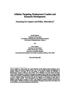
The first line in Equation (6) applies to situations when forecasters start the adjustment from the bottom because they estimate that inflation is below the target, Et −12π t < π t (forecasts are made 20 months ahead). The second line in Equation (6) refers to the cases where forecasters start the adjustment from the top because they think inflation overshot the target, Et −12π t > π t . Of note, the adjustment improves as A → 1 , in which case the range of uncertainty is shortened. The limit case A = 1 corresponds to full central bank credibility, which in our model is only asymptotically reached. The greater the credibility, the shorter the range of uncertainty, and the more accurate the adjustment toward the anchor. As such, it is not surprising that our A-index is strongly correlated with conventional “credibility indices” from the macroeconomic literature (see Figure 2 below). Figure 2 shows this correlation using the credibility index C suggested in Ref. [11]: E − πt 100 . C 100 − t −12 = 2
(7)
The anchoring index (6) is different for each forecaster. In the adaptive learning framework, there is no reason for assuming from the start that expectations are homogeneous. However, due to the feedback with the environment in the evaluation of past performance, learning allows the commuting of individual anchoring heuristics. The degree of heterogeneity in a given time period of the learning process can be gauged by a Pearson correlation, dividing the standard deviation by the mean. So the less the dispersion is between the individual forecasts on a given date, the greater the homogeneity of the forecasts. However, because the Pearson coefficient assumes the degree of heterogeneity is evaluated relative to the mean, it is useless in the presence of marked skewness. Fortunately, this restriction does not apply to our data, because we found the individual forecasts to be roughly symmetrically distributed (available upon request).
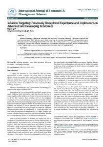
3. Results Figure 1 shows the inflation target and actual inflation for the time period considered. To measure the degree to which the inflation target was considered in the private forecasts, Figure 2 plots the anchoring index (6). The
Figure 1. Brazilian inflation target and actual inflation: November 30, 2001 to September 30, 2013.
Figure 2. Anchoring and credibility indices for November 30, 2001 to March 28, 2013.
OALibJ | DOI:10.4236/oalib.1101450
5
April 2015 | Volume 2 | e1450
E. Da Silva, S. Da Silva
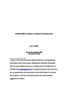
anchoring index gauges the usefulness of the announced target as a base rate and it co-varies with the credibility index (7). Figure 3 shows the calculated Pearson coefficients tracking the degree of expectation heterogeneity over time. For example, take the time span from 2003 to 2005 in Figure 3. The anchoring index dropped, and expectations became more heterogeneous than those of the final period (say, 2012 to 2013), but they were still less heterogeneous than those from the beginning (say, 2001 to 2002). Of note: On July 30, 2004 and March 28, 2013, the anchoring indices were roughly the same. But the fact that expectation heterogeneity was lower in the final period suggests forecaster learning was at play. When inflation accelerates, the central bank’s credibility plummets, and then the anchoring index drops. This means actual inflation becomes more relevant for forecasts than the target inflation. Here we arguably are in the second line of the A-index (6). The adjustment starts from the top and we expect it to stop well above the anchor given by the inflation target. As the private forecasters learn that actual inflation becomes a better predictor, expectations turn more homogeneous, and this reduces “inflation surprise” (actual minus expected inflation). Because the same actual inflation ends up generating less inflation surprise, this again strongly suggests an underlying process of learning at work. Take the final years in Figure 4, for example. Inflation surprise becomes tamed and the anchoring index shows a reduction. This means learning is improved (because inflation surprise is reduced), despite the fact that forecasters are relying less on the target (the anchoring index drops). Considering the constant-gain estimator given by Equation (1) into the PLM Equation (2), we can estimate
Figure 3. Learning at work: Expectation heterogeneity and anchoring index.
Figure 4. Both inflation surprise and the anchoring index progressively decrease. This means learning is improved without the need to rely on the target: November 30, 2001 to May 31, 2013. OALibJ | DOI:10.4236/oalib.1101450
6
April 2015 | Volume 2 | e1450
E. Da Silva, S. Da Silva
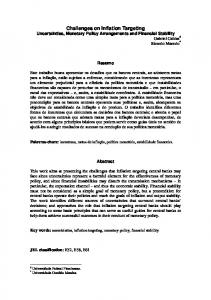
parameters µ and α (Table 2). Note that α < 1 in Table 2, thus satisfying the E-stability convergence condition (4). Calibrating the E-stability differential Equation (3) with the estimated parameters in Table 2, after considering the particular solution (5), we are certain that inflation forecasts do converge to an asymptotical equilibrium for the estimated α = −1.1 . Figure 5 shows a visualization of the convergence process toward the adaptive learning expectation equilibrium, which can be calculated as: = a 13.0333 (1 − ( −1.13594 ) )
−1
a = 6.101904.
Considering the inflation target of 4.5 ± 2 percent announced for the final period by the Brazilian central bank (Figure 1), we conclude the forecasters did not believe the core target of 4.5 percent. They expected 6.1 percent inflation, which is near the upper band of tolerance of 6.5 percent. The reason: lack of credibility in the announced target; increase in the range of uncertainty; and the resulting anchoring-heuristic adjustment starting from the top with a final estimate above the target. Importantly, when approaching the asymptotic value of 6.1 percent, the private forecasters succeed in reducing their forecasting error and subsequently in lowering the heterogeneity of their predictions. Of course, our adaptive learning equilibrium does not collapse to the rational expectation equilibrium. Table 3 presents the results of four tests commonly employed [12] to assess forecast rationality. Testing for bias (test A) is the simplest way to evaluate forecast accuracy. The test assess whether inflation expectations are centered on the “right” value. The accuracy is gauged by the constant ε regressed on the forecast errors (inflation surprise), π t − Et −12π t . A positive mean error indicates private forecasters are underestimating inflation. The magnitude 1.09 shown in Table 3 is large enough for one to reject the hypothesis of forecast accuracy without significant errors. This means forecasters, on average, showed significant forecast biases (errors). Test B evaluates whether there is information in the predictions that could be used to predict the inflation surprise. Accepting the null hypothesis of rationality means no other information conveys prediction power over inflation. The p-value of 0.015 shown in Table 3 means the null could not be accepted. Thus, the information conveyed by the expected inflation in the actual moment the forecasts were made was not completely exploited. Table 2. Actual law of motion of the Brazilian inflation: December 2001 to September 2013). Parameters of Equation (2)
µ 13.0333
α −1.1359*
*
Note: *significant at 1 percent.
Figure 5. Convergence to the adaptive learning equilibrium. This is the time window from the sample: November 30, 2001 to March 28, 2013. From the model’s Equation (5), we find a = 6.1 .
OALibJ | DOI:10.4236/oalib.1101450
7
April 2015 | Volume 2 | e1450
E. Da Silva, S. Da Silva Table 3. Tests of forecast rationality. Test A Testing for bias π t − Et −12π t = ε
ε : mean error (constant only)
1.09 (0.239348)*
Test B Is the information in the forecast fully exploited? π t − Et −12π t = ε + β Et −12π t
β
−0.38 (0.1564)**
ε
3.15 (0.8692)*
Adjusted R²
0.034
p-value
0.015
Test C Are forecasting errors persistent? π t − Et −12π t = ε + β (π t −12 − Et −24π t −12 )
β
0.961 (0.023)*
ε
0.02 (0.07)
Adjusted R²
0.925
Test D Are the macroeconomic data fully exploited? π t − Et −12π t = ε + β Et −12π t + γπ t −13 + κ it −13 + δ ut −13
ε
−0.973 (1.13)
β
−0.251 (0.193)
γ
0.064 (0.132)
κ
−0.348 (0.113)*
δ
0.888 (0.175)*
Adjusted R²
0.21
p-value
0 *
**
Note: Standard deviation in parentheses; significant at 1 percent; significant at 5 percent.
Test C assesses whether today’s forecast error can be used to predict tomorrow’s error (serial autocorrelation). If expectations are rational, serial autocorrelation cannot exist. Table 3 shows coefficient β = 0.961 significant at 1 percent. Thus forecasters presented error autocorrelation, which violated rational expectations. However, the fact that the forecast errors in t − 1 persisted in t is also compatible with objective, incomplete information rather than subjective, bounded rationality. This is because the realease of inflation data by the Brazilian authorities occurred with a one-month lag and even then, the errors were not entirely revealed. Test D examines whether public macroeconomic information was taken into account by forecasters in their predictions. The test runs a regression considering the expectations of current IPCA inflation rate formed with a 12-month lag Et −12π t , actual inflation π t −13 , an unemployment rate ut −13 and an interest base rate (called SELIC) it −13 , published in the month preceding the date when the forecasts were made (the series began in October 2001). Table 3 shows that the variables relative to the expectations of inflation were not statistically significant. However, the coefficient related to unemployment was positive and significant (δ = 0.888 ) . This value is considered high and implies that an increase in unemployment was followed by a reduction in inflation expectations for the next period, a pattern called “Phillips curve.” This, in turn, raised the forecast errors, which means an underestimation of the inflation forecasts during periods of growing unemployment. Finally, contractionary monetary policy (an increase in variable it −13 ) could not reduce the inflation forecasts, which means an OALibJ | DOI:10.4236/oalib.1101450
8
April 2015 | Volume 2 | e1450
E. Da Silva, S. Da Silva
overestimation and a negative forecast error.
4. Discussion When central banks adopt inflation targeting they create an illusion of the understanding of and control of inflation forecasts. They tend to understate the uncertainty of forecasting the future. The basic reason: They rely on models that assume the random shocks hitting the economies are independent and identically distributed. Jumps that lead to non-i.i.d. forecasts are dismissed by design, which means central banks assume economic shocks are of mild type I randomness [13]. However, this assumption is not rooted on the past evidence of inflation forecast behavior. Indeed, in interwar Germany, hyperinflation was fed by scalable inflation forecasts, a feature most macroeconomists and central bankers are aware of. As a consequence, the German currency moved from 3 to a dollar to 4 trillion to a dollar in just a few years during the 1920s. This is wild type II randomness [13]. Our finding of an asymptotic adaptive learning equilibrium that overshoots the anchor is thus dependent on both the adaptive learning model we consider as a framework [5], which assumes mild randomness, and the particular data used to calibrate the model, which did not present scalable inflation forecasts in the period considered. We took recent Brazilian data for the variable, not those of interwar Germany—the observation window was not large enough to include substantial deviations. Sums of i.i.d. finite variance random variables asymptotically approach a Gaussian distribution. Concepts, such as standard deviation, variance, correlation, R-square, and ordinary least squares, acquire meaning only if the environment is Gaussian [13]. The adaptive learning model we consider was designed within this environment of nonscalable randomness, and it is not surprising that “least squares learning” reaches an asymptotic equilibrium. So our result was obtained within this Gaussian environment. For this very reason the result is conservative because things could be even worse in a wild randomness environment. Here, inflation forecasts may not reach any fixed point equilibrium, as in the German example, and inflation targets end up useless.
5. Conclusions While predicting, forecasters may use simple heuristics (simple rules, usually imperfect, aiming to find answers to questions of difficult judgment). We consider this cognitive psychology perspective to the conventional macroeconomic literature of bounded rationality with adaptive learning and suggest the presence of an anchoring heuristic at work for predicting the inflation target. The treatment considered Brazilian data. Calibrating the data to the dynamic convergence of an adaptive learning asymptotical state, we found the professional forecasters to increasingly homogenize their forecasts, but the convergence value of the inflation expectation overshot the official announced target. We found that the forecasters didn’t believe the core target of 4.5 percent, and instead used a forecast of 6.1 percent inflation, which was near the upper band of 6.5 percent because the tolerance range was ±2 . This example spoils the very justification for inflation targeting because it shows the target is unlikely to work when private forecasters rely on anchoring heuristics.
References [1]
Bernanke, B.S. and Mishkin, F.S. (1997) Inflation Targeting: A New Framework for Monetary Policy? Journal of Economic Perspectives, 11, 97-116. http://dx.doi.org/10.1257/jep.11.2.97
[2]
Goncalves, C.E. and Salles, J.M. (2008) Inflation Targeting in Emerging Economies: What Do the Data Say? Journal of Development Economics, 85, 312-318. http://dx.doi.org/10.1016/j.jdeveco.2006.07.002
[3]
Ball, L. and Sheridan, N. (2003) Does Inflation Targeting Matter? NBER Working Paper No. 9577.
[4]
Thomas, L.B. (1999) Survey Measures of Expected U.S. Inflation. Journal of Economic Perspectives, 13, 125-144. http://dx.doi.org/10.1257/jep.13.4.125
[5]
Evans, G.W. and Honkapohja, S. (2001) Learning and Expectations in Macroeconomics. Princeton University Press, Princeton.
[6]
Conlisk, J. (1996) Why Bounded Rationality? Journal of Economic Literature, 34, 669-700.
[7]
Benveniste, A., Metivier, M. and Priouret, P. (1990) Adaptive Algorithms and Stochastic Approximations. SpringerVerlag, Berlin. http://dx.doi.org/10.1007/978-3-642-75894-2
[8]
Anufriev, M. and Hommes, C. (2012) Evolution of Market Heuristics. The Knowledge Engineering Review, 27, 255-
OALibJ | DOI:10.4236/oalib.1101450
9
April 2015 | Volume 2 | e1450
E. Da Silva, S. Da Silva 271. http://dx.doi.org/10.1017/S0269888912000161 [9]
Kahneman, D. (2011) Thinking, Fast and Slow, Farrar, Straus and Giroux. New York.
[10] Jacowitz, K.E. and Kahneman, D. (1995) Measures of Anchoring in Estimation Tasks. Personality and Social Psychology Bulletin, 21, 1161-1666. http://dx.doi.org/10.1177/01461672952111004 [11] Sicsu, J. (2002) Expectativas Inflacionárias no Regime de Metas de Inflação: Uma Análise Preliminar do Caso Brasileiro. Economia Aplicada, 6, 703-711. [12] Mankiw, N.G., Reis, R. and Wolfers, J. (2003) Disagreement about Inflation Expectations. NBER Working Paper No. 9796. http://dx.doi.org/10.2139/ssrn.417602 [13] Mandelbrot, B. and Taleb, N.N. (2010) Mild vs. Wild Randomness: Focusing on Those Risks That Matter. In: Diebold, F.X., Doherty, N.A. and Herring, R.J., Eds., The Known, the Unknown and the Unknowable in Financial Institutions: Measurement and Theory Advancing Practice, Princeton University Press, Princeton, 47-58.
OALibJ | DOI:10.4236/oalib.1101450
10
April 2015 | Volume 2 | e1450