International Journal of Scientific & Engineering Research, Volume 5, Issue 9, September-2014 ISSN 2229-5518
206
INFLATION TARGETING WITH DYNAMIC TIME SERIES MODELLING – THE NIGERIAN CASE Olanrewaju I. Shittu, Raphael A. Yemitan Abstract — In recent times, inflation figures used by policy makers and investors are usually at lag one (i.e. previous month’s inflation rate). The reality of the present day situation where changes in the economy increases with a high degree of uncertainty, decision of monetary policy tools requires the use of current figures of macroeconomic indicators such as inflation. This paper, therefore aims at modelling and forecasting Nigeria’s inflation rate for the current period, using the random walk with drift. The result will enable policy makers and investors determine inflation rate ahead of the time the official figures will be released. Our result shows that in the last 12months, there has been a high degree of correlation (99.8% ) between the forecast values and the official data from the National Bureau of Statistics. The results also indicate the need to study the long memory properties of the series. Index Terms— Consumers Price index, Inflation Targeting and Forecasting, Nigeria, Nigeria NBS, Random Walk
—————————— ——————————
1 INTRODUCTION
I
nflation measures the relative changes in the prices of commodities and services over a period of time. This economic indicator has a direct effect on the state of the economy. Around the world, keeping a strong control over Inflation has turned out to be one of the primary objectives of the regulators as inflation increases uncertainty in an economy. Inflation is an important economic indicator that the central banks, government, economist and other stakeholders use as their bases of argument when debating about the state of the economy. In recent times, the direction of the rate of inflation in an economy has largely influenced the decisions of policy marker, especially in Nigeria as seen in the 2012. Most economist and monetary policy authorities’ favor a low and steady rate of inflation. It reduces the severity of economic recessions by enabling the labor market to adjust more quickly in a downturn. More precisely, it reduces the cost of borrowing by manufacturers which lower their cost of input and boost their profitability. Also, it generally improves investment in the economy which in turn reduces unemployment and increase economic output. In Nigeria, the Monetary Policy Committee (MPC) of the Central Bank of Nigeria (CBN) has taken a contractionary stance on its monetary policy tools for 28 calendar months (September 2010 - January 2013) to check inflationary threats. The primary objective of MPC are to control inflation and maintain a stable exchange rate environment by use of the monetary policy tools, such as many experts and stakeholders in Nigeria are currently advocating for an easing in the MPC stance to enable growth. But with the time lag (1-month) between announcement of the monthly inflation figures and the MPC meeting, it’s difficult for policymakers to properly coordinate their strategy. In such circumstances, statistical forecasts and estimates can assist policy markers in formulat-
ing their strategies. Methodologies in literatures for Nigeria’s macroeconomic variables have not accurately helped in this area as a result of certain misconceptions on the choice of the appropriate tools and procedures for real time decision making. We investigate the intrinsic nature of the Nigerian Inflation rate were that successive observations are dependent or correlated. Time series analysis studies the stochastic mechanism of an observed series. The study of time series, especially the univariate time series Auto Regressive Integrated Moving Average (ARIMA) models, helps to understand and describe the underlying generating mechanisms of an observed series. This analysis assists in forecasting future values and can be very valuable when formulating policies for development. Increase in inflation can be influenced by many factors. The prime cause of inflation can vary from month to month as seen in the final months of 2012. The possible factors behind excessive inflation can include supply side factors including cost push relationship along with exchange rate effects, excessive borrowing by the government and demand pull inflation. Hence, successful execution and influence of monetary policy in any economy largely depends on the efficiency and accuracy of forecasting macroeconomic variables like inflation.
IJSER
————————————————
• Olanrewaju I. Shittu is currently an associate professor in statistics at the University of Ibadan, Ibadan, Nigeria. E-mail:
[email protected],
[email protected] • Raphael A. Yemitan is currently pursuing a PhD degree program in statistics at the University of Ibadan, Ibadan, Nigeria, PH-2348055455396. Email:
[email protected],
[email protected]
As the economic effect of monetary policy have time lag policy makers and financial authorities require frequent updates to the path of inflation. Policy makers can get prior indication about possible future inflation through Inflation forecasting using different statistical methodologies. In this paper, the Nigerian Consumers Price Index (CPI) between January 2008 and December 2012 is used to make appropriate predictions for the next 12 months (January to December 2013) using only information gathered from the data. The structure of the paper is as follows: Section 1 introduces the work; section 2 reviews available literatures on the subject matter; Section 3 presents the methodology for approaching the work. Section 4 [resents the analysis of results and discussion while the concluding remarks are given in Section 5.
IJSER © 2014 http://www.ijser.org
International Journal of Scientific & Engineering Research, Volume 5, Issue 9, September-2014 ISSN 2229-5518
2 LITERATURE REVIEW Based on [1] notion of stochastic process in time series by postulating that every time series can be regarded as the realization of a stochastic process, a number of time series methods have been developed. Among the developed time series methods was the major contribution by [2]. They introduced univariate models for time series which simply made systematic use of the information included in the observed values of time series. This offered an easy way to predict the future movement of a variable through a coherent, versatile threestage iterative cycle for time series identification, estimation, and verification. [2] had enormous impact on the theory and practice of modern time series analysis and forecasting. [3], also worked on the autoregressive and moving average models have been greatly favored in time series analysis. In general, time series variables in economics and finance are usually stochastic and frequently non-stationary, such series from literature include stock prices, gross domestic product (GDP), consumer price index (inflation rate) etc. This series are generally modeled by either trend or difference stationary process. A trend stationary process of the form, y t = f(t) + e t , where t is the time and f(t) is a deterministic function and et is the random shock. The stochactic term in a trend stationary process is stationary and has no stochastic drift which can be removed from the data by difference stationary process to, yt = y t-1 + c + e t , where c is a non-stochastic drift parameter: even in the absence of the random shocks et, the mean of y would change by c per period and y t-1 is the first lag of y t . As in the case of a trend stationary process, the non-stationarity can be removed by differencing, usually the differenced series of the form, z t = y t - y t-1 . The difference series will have no drift parameter due to the absences of a long-run mean parameter c. The absences of the drift parameter notwithstanding, this unit root process exhibits stochastic drift due to the presence of the stationary random shocks et. The relevance of this in our context of inflation and monetary policy is to help the central banks’ to determine if they should attempt to achieve a fixed growth rate in consumer prices for each time period i.e. difference stationary, or for them to target a return of prices to a predetermined growth path i.e. trend stationary. In the later, no price level is allowed to drift from the predetermined path, while the in the former, any stochastic change in prices affects the expected values of consumer prices along its future path. In both cases, price level drift as a function of increasing expected value but differ based on non-stationarity.
207
several univariate models. This include the AR(p) and the random walk. Similarly, [7] made use of simple time series models to compare inflation forecasts from the Riksbank. Also, [8] as well as [9] also considered ARMA models to construct forecasts for Chilean inflation and GDP growth respectively while[10] in a working paper for the Central Bank of Chile explored the Driftless Extended Seasonal AIMA (DESARIMA) against the traditional univariate time-series benchmarks available in literature.
In Nigerian, there have been a number of studies on forecasting inflation using several time series techniques. [11] and [12] in their works imposed an ARIMA (1,0,0) on the Nigerian inflation rate with a view of establishing the model fit and adequacy. The work by [13] also concluded with the efficiency of the ARIMA model. Other related works on Nigeria’s Inflation include [14] and [15]. Their conclusion only suggested the relatively good nature of the ARIMA model and advised its use as a benchmark for other models without forecasting. Interestingly, the work of [12] attempted to forecast Nigeria’s inflation rate for 2012 and concluded that the series followed a (1, 1, 0)x(0, 1, 1)12 model but the forecasts were approximately 2% to 2.5% lower than the official rate of inflation in 2012.
IJSER
The use of different univariate time series models to generate forecasts is common in the literature and in forecasting inflation in particular. [4] show that a simple variation of a random walk model for the Year-on-Year (YoY) inflation in the United States is very competitive when predicting inflation 12-months ahead. [5] also for the United States, presented an empirical application in which several CPI forecasts are compared to those generated by a random walk with drift, an autoregression in which the lag length is selected using the Bayesian Information Criteria (BIC). In the UK, [6] evaluated the accuracy of the Bank of England inflation forecasts using
3 METHODOLOGY
Forecasting inflation rate using the CPI as input can be achieved through structural and statistical modeling. Structural models are based on economic theory; however, the complex link between economic variables is in general difficult to describe accurately leading to a cumbersome system of equations. However, statistical models by their nature offer very little economic logic, but great mathematical/statistical reasoning exclusively from the past behavior of the series. The statistical modeling approach is used in this paper.
Despite the black box reputation of the statistical model as a result of the lack of additional information, typically provide relatively good results in their primary task – forecasting. An intrinsic problem when applying ARIMA class models, and all stochastic models, to a macroeconomic series is that they are, by their nature, short, with frequent changes in structure, and contain changeable and sometimes unclear composition (most times seasonality). This is particularly true when applied to most Nigerian macroeconomic series, so, when developing CPI forecast models, we pay particular attention to the data structure, the model’s characteristics and also models out-ofsample characteristics (quality of forecast).
3.1 ARIMA Model Building Building ARIMA(p,d,q) model involve a number of steps. The first and most important step is the model identification. This involves the studying the Autocorrelation Function (ACF) and Partial Autocorrelation Function (PACF) of the data in order to examine the stationarity of the data which is a necessary condition for ARIMA(p,d,q) modeling. It also gives an idea of the type of ARIMA(p,d,q) model suitable for the data. This all important step can be referred to as model identifi-
IJSER © 2014 http://www.ijser.org
International Journal of Scientific & Engineering Research, Volume 5, Issue 9, September-2014 ISSN 2229-5518
cation. After model identification, the next step is model estimation with efficient software’s, using either the least squares or maximum likelihood methods to estimate the parameters of the model. The next step is the model diagnostic, which is a procedure to verify whether or not the model is a good fit. If the model is not a good model then re-specify and estimate again. The final step is the forecasting after which a meta diagnostics is carried out to verify the forecast ability of the model. Detailed explanation of dynamic modeling can be found in Box and Jenkins (1976), Mills (1990) and Hamilton (1994).
If a model is rejected at this stage, the model-building cycle has to be repeated. Note: This test only make sense if k > p + q. •
3.2.1 •
p+q n
where σˆ 2 is the estimated variance of e t . •
Schwarz's Bayesian Information criterion (SC, BIC, or SBC):
BIC = log σˆ 2 + 2
p+q log(n) n
Both criteria are likelihood-based and represent a different trade-off between "fit", as measured by the loglikelihood value, and "parsimony", as measured by the number of free parameters, p + q. If a constant is included in the model, the number of parameters is increased to p+q+1. Usually, the model with the smallest AIC or BIC values are preferred. While the two criteria differ in their trade-off between fit and parsimony, the BIC criterion can be preferred because it has the property that it will almost surely select the true model.
∑ (Yt − Y )(Yt −k − Y ) cov(Yt Yt −k ) ACF (k ) = t =1+ k = var(Yt ) ∑ (Yt − Y ) 2 t =1
Partial Autocorrelation function (PACF): The PACF measures the additional correlation between Y t and Y t-k after adjustments have been made for the intermediate values Y t-1 ,…, Y t-k+1 . The PACF is closely related to ACF, their value also lies between -1 and +1. The specific computational procedures for PACFs are complicated, but these formulas do not need to be understood for us to use PACFs in the model identification phase Diagnostics: In the model-building process, if an ARIMA(p, d, q) model is chosen (based on the ACFs and PACFs), some checks on the model adequacy are required. A residual analysis is usually based on the fact that the residuals of an adequate model should be approximately white noise. Therefore, checking the significance of the residual autocorrelations and comparing with approximate two standard error bounds, i.e. 2/sqrt(n) are needed Ljung-Box (1978) statistics: Q-statistics is an objective diagnostic measure of white noise for a time series, assessing whether there are patterns in a group of autocorrelations.
Criteria for model selection Akaike's information criterion (AIC):
AIC = log σˆ 2 + 2
3.2 Identification: ARIMA Model Identification Tools Graph plots such as correlogram are used as part of a model selection process. The correlogram consist of autocorrelations’and partial autocorrelations’displayed either as a table of values of most often as a plot of the coefficients. • Autocorrelation function:
•
208
IJSER
ACF (i ) 2 N(k-p-q) − i degree of freedom 1 for i= 1 to ki =with K
Q = n(n + 2)∑
Ho: ACFs not significantly different than white noise ACFs (i.e., ACFs = 0). H1: ACFs statistically different than white noise ACFs (i.e., ACFs ≠ 0). Decision rule: • If Q ≤ chi-square table, No reject Ho, the ACF patterns are white noise • If Q > chi-square table, Reject Ho, the ACF patterns are not white noise
3.3 Stationarity Test The non-stationarity or otherwise of a series can strongly influence its behavior and properties. Various definition of non-stationarity exists but we consider the weak form or covariance stationarity. Non-stationarity is often characterized mainly by two models, the random walk with drift model and the deterministic trend process. • Random walk with drift y t = µ + y t-1 + e t • Deterministic trend process yt = µ + β t + et Where e t is iid in both cases. To verify the existence of a unit root in process, the test H 0 : β = 1 versus H a : β< 1using either of the models above. The two models require different treatments to induce stationarity; the Dickey Fuller and Augmented Dickey Fuller (ADF) tests amongst others. In this paper we considered the augmented dickey fuller test. 3.3.1 Augmented Dickey Fuller Test Augmented Dickey–Fuller test is a an augmented version of the Dickey–Fuller test used to verify a unit root in a time series sample. Using the regression p −1
y t = ct + βy t −1 + ∑ φ i ∆xt −i ... + et i =1
Where c t is a deterministic function and ∆x t −i = x t − x t −1 is the
IJSER © 2014 http://www.ijser.org
International Journal of Scientific & Engineering Research, Volume 5, Issue 9, September-2014 ISSN 2229-5518
differenced series of ratio of
xt . The ADF test statistic is given by a t-
βˆ − 1 , ADF − test =
Where
βˆ − 1 std ( βˆ )
209
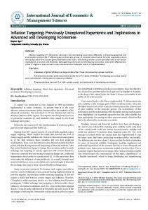
been smoothen out bythe other component. However, a look at the time plot indicates that we cannot categorically rule out the existence of a trend component from the series. Our suspicion of non-stationarity is further strengthened by the ACF and the PACF of the data as in Figure 2.
βˆ is the least square estimate of β and stationarity if
ACF for index 1
determined by the hypothesis H 0 : β = 1 versus H a : β< 1
+- 1.96/T^0.5
0.5 0
The non-stationarity or otherwise of a series can strongly influence
-0.5 -1
0
2
4
6
8
10
12
14
16
lag
4 DATA ANALYSIS AND RESULTS
PACF for index 1
4.1 Data Summary The data used are the monthly Nigerian Consumers Price Index (CPI) between January 2008 and December 2012 to make appropriate predictions for the next 12 months (January to December 2013) using only information gathered from the data. The data between January 2012 and May 2013 are used to test the efficiency and reliability of our model. Data was collected from the National Bureau of Statistics NBS monthly CPI reports.
+- 1.96/T^0.5
0.5 0 -0.5 -1
0
2
4
6
8
10
12
14
16
lag
Fig. 2. Correlogram (ACF and PACF)
IJSER
In an immense empirical exercise to accurately predict the TABLE 1 DATA SUMMARY Variable cpi
Mean 128.185
Median 128.100
Minimum 109.900
Maximum 146.600
Variable cpi
Std. Dev. 11.5759
C.V. 0.0903064
Skewness 0.0298947
Ex. kurtosis -1.36855
The ACF decays slowly to zero, indicating non stationarity of the data while the PACF cuts of after lag 1. The next step is to investigate the level of non-stationarity in the data with the use of Augmented Dickey Fuller Test (ADF).
4.2 Unit Root test (Augmented Dickey fuller Test) The data according to the ADF test result (Table 2) shows that the CPI data is non stationary. However, after first difference (Table 2) the ADF reveals the CPI data becomes staionary
TABLE 2 AUGMENTED DICKEY-FULLER (ADF) TEST FOR CPI including 10 lags of (1-L)CPI (max was 10) sample size 53 unit-root null hypothesis: a = 1 test with constant 𝑝−1 Model yt = β0 + a*yt-1 +∑𝑖=1 𝜙𝑖 Δ𝑥𝑡−𝑖 ... + e
Fig. 1. Tiime plot of Nigeria’s CPI (2009=100)
1st-order autocorrelation coeff. for e
Nigerian Inflation rate for the year 2013, there are a number of interesting findings that deserve mentioning. We organize our discussion around four major topics: model Identification, estimation, diagnosis and forecast.
-0.061
lagged differences
F(10, 41) = 1.498 [0.1750]
Estimated value of (a - 1)
0.0106474
Test statistic: tau_c(1) =
1.39366
asymptotic p-value
0.9991
At first glance, the Time Plot (figure 1)of the CPI shows the series exhibits non-stationarity with drift and slope. Obviously, the series is non-seasonal from the shape of the time plot this issurprising because it is believed that the rate of inflation is correlated with the agricultural seasons in Nigeria. Since the data used is the aggregate CPI.The effect of season could have IJSER © 2014 http://www.ijser.org
International Journal of Scientific & Engineering Research, Volume 5, Issue 9, September-2014 ISSN 2229-5518
TABLE 3 AUGMENTED DICKEY-FULLER (ADF) TEST FOR FIRST DIFFERENCED CPI
including 10 lags of (1-L)CPI_1 (max was 10) sample size 53 unit-root null hypothesis: a = 1 test with constant 𝑝−1 Model yt = β0 + a*yt-1 +∑𝑖=1 𝜙𝑖 Δ𝑥𝑡−𝑖 ... + e 1st-order autocorrelation coeff. for e
-0.067
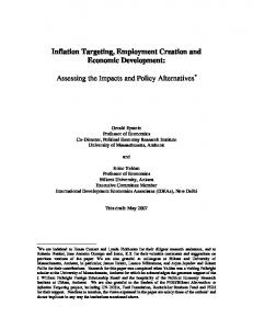
Fig. 3. Differenced lagged differences Nigeria’s CPI
F(2, 56) = 3.041 [0.0557]
Estimated value of (a - 1)
-1.23089
Test statistic: tau_c(1) =
-5.71416
asymptotic p-value
5.6757e-007
210
government of Nigerian partially removed the fuel subsidy it pays to marketers of petrol. The model in such unexpected situations, captures the shocks after a month lag and forecast the subsequent months effectively. In addition the correlation coefficient returns a 99.8% relationship between the NBS offiTABLE 4 ARIMA (0,1,0) OR RANDOM WALK WITH DRIFT MODEL MODEL
Model : ARIMA, using observations 2008:02-2012:11 (T = 58) Dependent variable: (1-L) index coefficien std. error z p-value const 1.05 0.1155 9.0907 9.84E-20*** Mean dependent var 1.05 S.D. dependent var 0.8796 Mean of innovations 6.13E-17 S.D. of innovations 0.8796 Log-likelihood -74.3562 Akaike criterion 150.71 Schwarz criterion 152.7729 Hannan-Quinn 151.52 Fig. 4. Actual, Fitted and Forecast of the CPI
After the first difference (figure 3), the series becomes stationary. As a result of the non-seasonal appearance and stationarity of the series at first difference, we suspect an ARIMA(0,1,0) model called the random walk with drift model as a result of the linear growth behavior. To confirm suspicion, we used the autocorrelation and partial autocorrelation functions to identify the model. As we rightly suspected, the correlogram (Charts of the ACF and PACF in figure 3) confirms the series is a random walk with drift model (this conclusion was made based on the correlogram graph plot rule given above).
TABLE 5 NORMALITY TEST
IJSER
4.3 Selected Model Estimation and Forecast Table 4 shows the estimated random walk with drift model. Table 5 and Figure 4 shows the model adequacy/residual test; this is required when the correlogram is used to determine a model and model order. The residual analysis shows that the residual of the random walk with drift model is a white noise since the Q statistics p-value is significant at 95% level of significance, i.e. 0.019≤0.05. A plot of the actual against the fitted series (figure 5) shows an approximately equal series. Also the estimated coefficient (const) of the series in table 4 is significant at the 99% level of significance. Hence, we have a good forecasting model for the Nigerian CPI. The result of the CPI forecast (figure 4) show the goodness of fit statistics R2 of the fitted series fits the actual series by 99.6%. The result of the reduced data to establish the consistency of the random walk with drift model also gives an approximately the same result with the official released series in 2011 (Appendix 1 Table 3). Hence, we believe that with all things been equal the forecast for the Nigerian CPI using the random walk with drift model will be very useful for policy makers, especially the MPC and the CBN in making policy decisions relating to the position of the Nigerian inflation rate. In addition, it is worth noting that in the event of an unexpected short as experienced in January 2012 when the federal
Frequency distribution for uhat2, obs 2-59 number of bins = 7, mean = 6.12537e-017, sd = 0.879643 intervalmidpt frequency rel. cum. < -1.25 -1.65 2 3.45% 3.45% * -1.2500 - -0.45 -0.85 19 32.76% 36.21% *********** -0.45000 - 0.35 -0.05 19 32.76% 68.97% *********** -0.35 1.15 0.75 14 24.14% 93.10% ******** -1.15 1.95 1.55 1 1.72% 94.83% -1.95 2.75 2.35 2 3.45% 98.28% * >= 2.75 3.15 1 1.72% 100.00% Test for null hypothesis of normal distribution: Chi-square(2) = 8.494 with p-value 0.01431
cial CPI and the model forecast, showing the level of reliability of the model After the forecast on the CPI, we computed the inflation rate using the fitted data and the forecast to show the rate of inflation in the review period. Inflation rate is calculated on year on year basis s the rate of increase or change in the general consumer price level from the same of the previous year. This is described s follows;
Inflation Jan , 2013 =
(CPI Jan , 2013 − CPI Jan , 2012 ) CPI Jan , 2012
* 100%
Where CPI Jan,2013 represent the January 2013 CPI forecast and CPI Jan,2012 is the official CPI for January 2012. Our result was, approximately the same with the actual figures reported by the NBS within the period (see figure 5).
IJSER © 2014 http://www.ijser.org
International Journal of Scientific & Engineering Research, Volume 5, Issue 9, September-2014 ISSN 2229-5518
211
REFERENCES
5 SUMMARY AND CONCLUSION In this paper, the univariate forecasting models were introduced and the procedure to follow in order to achieve optimum result from the use of the models. Our out-of-sample forecast clearly reveals the efficiency of the ARIMA models in forecasting macro-economy variables. The most important step we took was to allow the data direct our choice of model. We strongly believe and advise that making statistical predictions for decision making at every level, especially for monetary policy decision making by the MPC in Nigeria, the data should be allow to guide the prediction process. Our conclusions are on the result of our forecast compared to the official figures released by the NBS between 2008 and 2012. It should also be noted that the random walk with drift model is restricted to Nigeria’s CPI data series only and using it for other series may result in unpleasant results. As such, every data frame and variable to be forecasted for decision making should be studied using the ARIMA models or any other model as dictated by the data
[1] Yule, G.U. (1927). On a method of investigating the periodicities of disturbed series, with special reference to Wolfer's sunspot numbers. Philosophical Transactions of the Royal Society (A), 226, 267-298. [2] Box G.E.P. and Jenkins G.M., 1970 Time Series Analysis: Forecasting and Control, Holden-Day, San Francisco [3] Yule, G.U. 1921. On the time-correlation problem, with special reference to the variate-difference correlation method. Journal of the Royal Statistical Society 84, July, 497–526. [4] Andrew Atkeson & Lee E. Ohanian., 2001. "Are Phillips curves useful for forecasting inflation?," Quarterly Review, Federal Reserve Bank of Minneapolis, issue Win, pages 2-11 [5] Giacomini, R., and White, H. (2006), “Tests of Conditional Predictive Ability.” Econometrica 74, 1545-1578 [6] Jan J. J. Groen & George Kapetanios & Simon Price, 2013. "Multivariate Methods For Monitoring Structural Change," Journal of Applied Econometrics, John Wiley & Sons, Ltd., vol. 28(2), pages 250-274, 03 [7] Andersson, M.K., G. Karlsson & J. Svensson, (2007), ”The Riksbank’s Forecasting Performance”, Sveriges Riksbank Working Paper Series, forthcoming. [8] Groen, Jan J.J. & Kapetanios, George & Price, Simon, 2009. "A real time evaluation of Bank of England forecasts of inflation and growth," International Journal of Forecasting, Elsevier, vol. 25(1), pages 74-80 [9] Pablo Pincheira, 2010. "A Real Time Evaluation of the Central Bank of Chile GDP Growth Forecasts," Working Papers Central Bank of Chile 556, Central Bank of Chile.
IJSER
In particular, we suggest that the MPC of the CBN, should consider using such statistical models on key macroeconomic indicators to make specific decision on its monetary policy tools. This is because the variables use to make this decisions are usually late (i.e. 1-month to 3-months lag depending on the variables). Future investigations on the appropriate procedures and models for the other macro-economic series, espeTABLE 6 2013 NIGERIA’S INFLATION RATE FORECAST Model Forecast Year (%) Jan-13 9.1 Feb-13 9.6 Mar-13 8.7 Apr-13 9.1 May-13 9.1 Jun-13 8.5 Jul-13 8.8 Aug-13 8.6 Sep-13 7.8 Oct-13 7.8 Nov-13 7.9 Dec-13 7.9 Average 8.6
NBS actual (%) 9.0 9.5 8.6 9.1 9.0 8.4 8.7 8.2 8.0 7.8 7.9 8.0 8.5
cially Nigeria’s series’, seem to be interesting topics to consider and explore in subsequent research.
[10] Pablo Pincheira & Carlos Medel, 2012. "Forecasting Inflation With a Random Walk," Working Papers Central Bank of Chile669, Central Bank of Chile. [11] Adeola, J.O., 2012 Modeling On Inflation Rate in Nigeria Using ARIMA Model, http://journal.unaab.edu.ng/publicationsabstract/modeling%20on%20inflation%20rate%20in%20nige ria%20using%20arima%20model%20(a%20case%20study %20of%20central%20bani%20(%20of%20nigeria).pdf [12] Etuk, E.H., 2012. Predicting inflation rates of nigeria using a seasonal box-jenkins model. Journal of Statistical and Econometric Methods 1(3): 27-37 [13] Olajide J.T, Ayasola O.A, Odusina M.T and Oyenuga I.F, 2012, Forecasting the Inflation Rate in Nigeria: Box Jenkins Approach, IOSR Journal of Mathematics (IOSM-JM), Vol. 3, Issue 5(Sep-Oct. 2012), Pp 15-19. [14] Mordi C.N.O. et al, 2007, The dynamics of Inflation in Nigeria, Research Department, CBN Occassional Paper No. 32. [15] Alnaa, S., & Ahiakpor, F. (2011). ARIMA (autoregressive integrated moving average) approach to predicting inflation in Ghana. Journal of economics and international finance,3(5),(228-336). [16] Alnaa, S., & Ahiakpor, F. (2011). ARIMA (autoregressive integrated moving average) approach to predicting inflation in Ghana. Journal of economics and international finance, 4(3),83-87.
IJSER © 2014 http://www.ijser.org