Aug 8, 1995 - tween the cavitation event rate and the concentration of cavita- tion nuclei in ... In this paper, we first present the experimental observations of.
Zhenhuan Liu Graduaie Student.
Christopher E. Brennen Professor. Division of Engineering and Applied Science, Ca:ifornia Institute of Technology, Pasadena, CA 91125
Cavitation Nuclei Population and Event Rates To model the processes of cavitation inception, noise and damuge, it is necessaty to generate a model of the cavitation event rate which can then be coupled with the consequences of the individual events to produce a complete synthesis of thephenomenon. In this paper we describe recent efforts to connect the observed event rates to the measured distributions of cavitation nuclei in the oncoming stream. Comparisons are made between the observed event rutes and event rates calculated porn measured nuclei distributions using an algorithm which includes the dynamics of the nuclei motion and growth. Various complications are explored including the effect of the boundury layer, the relative motion between the nucleus and the liquid, the observable bubble size effect, and the eflect of bubble growth on neighboring nuclei. All of these are seen to have important influences on the event rate, and therefore, on cavitation inception and other macroscopic consequences. We demonstrate that it is possible to predict the correct order of magnitude o f the event rate when an attempt is made to model the important flow complications.
1 Introduction In order to synthesi~ethe cumulative effects of a stream of traveling cavitation bubbles, it is necessary to supplement the details of individual events with the ratcs at which these events occur. Many investigators have anticipated a relationship between the cavitation event rate and the concentration of cavitation nuclei in the oncoming stream (see, for example, Schiebe, 1972; Keller, 1972, 1974; Keller and Weitendorf, 1976; Kuiper, 1978; Gates and Acosta, 1978; Meyer et al., 1992). At first sight this seems like a straightforward problem of computing the flux of nuclei into the region for which C, < -a. However, many complications arise which make this analysis more difficult than might otherwise appear and we shall discuss some of the specific issues below. But these difficulties do not account for the lack of experimental research into the relationship. Rather, the difficulties involved in the accurate measurement of the incoming nuclei number distribution function, N(K). have been responsible for the delay in any detailed, quantitative invcstigation of this component of the problem. (Note that N(R)dR is the number of nuclei with size betwecn R and R + dR per unit volume.) As Billet (1985) remarked in his review of nuclei measurement techniques, the only reliable method of obtaining N(R) has been the extremely time-consuming procedure of surveying a reconstruction of an in situ hologram of a small volume of tunnel water (Gates and Bacon, 1978). However, the time and effort required to construct one N(R) distribution by this method has seriously limited the scope of these investigations. The recent development of light scattering instruments employing phase Doppler techniques (Saffman et al., 1984; Tanger et al., 1992) has improved the situation. In our laboratory, we have succeeded in validating and calibrating a Phase Doppler Anemometer (PDA) made by Dantec by taking si~ultaneous measurements with the PDA and a holographic system (Liu el al., 1993). The great advantage of the PDA system is the speed with which N ( R ) can be measured. After validation, the PDA system could then be used with coniidencc for investigations of the nuclei population dynamics in a water tunnel (Liu et al., 1993 and 1994) and of the aforementioned relation between Conmbuted by the Fluids Engineering Division for publication in the JOURNAI. R.uros ENOLVFBRING. Manuscript received by the Fluids Engineering Division August 8, 1995; revised manuscript received October 2, 1997. Associate Technical Editor: J. Katz.
OF
728 1 Vol. 120, DECEMBER 1998
N(R) and the cavitation event rate (Liu et al., 1993, Liu and Brenncn, 1994). In this paper, we first present the experimental observations of cavitation event rates on a Schiebe headfom with simultaneous measurement of the nuclei distribution in the upcoming stream. We then present an analytical model to synthesize the event rates from the measured nuclei distributions. Then we compare the predicted event rates with cavitation observations in two water tunnels with quite different nuclei population dynamics.
2 Observations of Nuclei Population and Event Rates The experiments were performed in the Low Turbulence Water Tunnel (LTWT) and the High Speed Water Tunnel (HSWT) at Caltech. Detailed descriptions of these two water tunnels a n be found in other literature (see Gates, 1978 and Liu and Brennen, 1995), and will not be repeated here. Figure I shows a sketch of the experimental setup. A Schicbc headfonn with 5.08 cm diameter was installed at the center of thc water tunnel. The free-stream nuclei number distribution was measured by a Phase Doppler Anemometer (PDA), which was calibrated by comparing the results with those obtained by a holographic method (Liu et al.. 2993). On the other hand, the cavitation event rate on the Schiebe headform was measured by three flush-mounted electrodes on the headform surface (Ceccio and Brennen, 1992 and Kuhn de ChizeUe et al., 1992). In Fig. 2, we present a typical comparison of the nuclei number density distributions in the LTWT and in the HSWT. Also plotted in the figure are measurements in other facilities (Arndt and Keller, 1976; Peterson et al., 1972, 1975; Fcldberg and Shlemenson, 1971; Keller and Weitendorf, 1976; and Gates and Bacon, 1978) and in the ocean (Cartmill and Su, 1993). As expected, substantial differences in the nuclei number density distributions in the two water tunnels were found. Although the shapes of the distributions are similar, the differences in the magnitudes were as much as two orders of magnitude. The typical nuclei concentration in the LTWT is quite large, about 100 ~ m - while ~ ; the nuclei concentration in the HSWT is low at about 1 cm-'. Billet (1985) and Gindroz and Billet (1994) presented useful reviews of the subject of nuclei concentralions and distributions. Thcy found that for deaerated water, typical concentrations are of the order of 20 cm with sizes ranging from about 5 pm to about 20 pm. We conclude that the LTWT is nuclei rich and the HSWT is nuclei poor. This was expected
Copyright O 1998 by ASME
Transactions of the ASME
PDA signal
,!Dlfirmeiver
1o5I lo4
. ..
. . . .....I . . . ...J
lo4 lo4 BUBBLE RADIUS, m
106
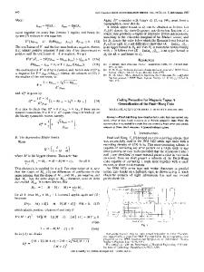
Fig. I Experimental setup for the simultaneous measurement of the cavitation nuclei distribution in the water tunnel and the cavitation event rate on a Schiebe headform
Fig. 2 A comparison of the nuclei number density distributions in the Low Turbulence Water Tunnel and the High Speed Water Tunnel with measurements in other facilities and in the ocean. The uncertainty in the ordinate is r 5 percent.
since the HSWT has an effective resorber while the LTWT does not; related studies (Liu, 1995, Liu et al., 1993) demonstrated that, as a result, the two facilities have quite different nuclei population dynamics. Consequently, comparative experiments in the two tunnels were expected to provide a valuable range of nuclei populations. Figure 3 presents the measurements of the event rates on a Schiebe headform in the LTWT and HSWT tunnels. Note that the cavitation event rates increase dramatically as the cavitation number is decreased. However, the event rates can vary by as much as a decade at the same cavitation number. At the same cavitation number, the larger free stream nuclei concentrations correspond to the larger cavitation event rates. As one would expect, the event rates observed at the same cavitation number in the LTWT are much higher than in the HSWT, because of the much higher nuclei population in the LTWT.
During the tests in the HSWT, cavitation experiments were performed at various speeds and air contents. Again, it was clear that the nuclei population had a strong effect on the cavitation event rate as illustrated on the right in Fig. 3. This resulted in a significant effect on the cavitation inception number. For example, at a velocity of 9.4 mls and a nuclei concentration of 0.8 cm-', the cavitation inception number was 0.47. After air injection, the nuclei concentration rose to 12 cm ', and cavitation inception occurred at u, = 0.52. In contrast, in the LTWT, the cavitation inception number in the LTWT was about 0.57, and the nuclei concentration was about 100 ~ m - In~ the . HSWT, attached cavitation occurred soon after traveling bubble cavitation. This implies that attached cavitation occurs more readily when the nuclei population is low. Similar phenomenon was also observed by Li and Ceccio ( 1994) on a cavitating hydrofoil. In their observations, when the nuclei concentration in the
Nomenclature C = nuclei concentration Cp = coefficient of pressure, ( p pm)l;pu2
-
CpM= minimum Cp on a given streamline CpMs= minimum value of Cp on the headform surface C& = constant D = headform diameter E = cavitation event rate N(R) = nuclei density distribution function R = radius of a cavitation nucleus R , R = d ~ i d t d, 2 ~ i d t 2 Rc = critical cavitation nucleus radius RM= minimum observable bubble radius R, = maximum cavitation bubble radius Ro = initial nucleus radius S = surface tension U = upstream tunnel velocity U.w = maximum velocity corresponding to CpMs
Journal of Fluids Engineering
fi ,h, .fi = numericaI factors effecting the cavitation event rate n, = bubblelbubble interaction effect p = fluid pressure p, = free stream pressure p,, = initial gas pressure in a bubble p, = blake critical pressure p, = undisturbed liquid pressure p, = vapor pressure q = flow velocity r = distance from the center of a bubble rH = headfonn radius r, = radius of curvature of streamlines near minimum pressure point rs = radius of minimum pressure point re = critical radius y = distance normal to body surface yM= maximum y value of the Cp = - u isobar
a streamline and the location of minimum pressure point t, = time available for bubble growth u , UM = fluid velocity, fluid velocity just outside boundary layer u = velocity of a bubble normal to streamline p = fluid density 0 = cavitation number, ( p , - p,)l s, so = coordinate along
uZ uc,= threshold cavitation number
a, = inception cavitation number a: = cavitation number variation E, X = factors in the chosen analytical expression for N(R) v = kinematic viscosity of fluid p = fluid viscosity 6, S2 = thickness and momentum thickness of the boundary layer E = displacement of a bubble normal to a streamline C = function defined by Eq. ( 15) = dZld(r/rH)
z'
DECEMBER 1998,Vol. 120 1 729
lo3 -
I
I
j
U (mlsec) (A) (B) (C)
,-
(D) (E)
'0
% lo2:
8.1 9.4 9.4 12.6 14.5
3.6 < C < 4.3 cm-3 C = 0.8 cm-3 1.7cCc2.4cm-3 2.0 < C < 3.0 cm-3 1.6 < C < 2.9 cm8
-
CAVITATION NUMBER, o CAVITATION NUMBER, o Fig. 3 Left: Variations in the cavitation event rates with cavitation number on a 5.08 cm Schiebe body in the L W at a speed of 9 mls. Data are plotted for various ranges of free stream nuclei concentration, C ( c W 3 ) :C < 150 (0); 150 < C < 200 (+); 200 < C < 250 (0)and 250