Felix BieÃmann, Cornelius Raths. Suzanne Martens. Jason Farquhar, Jeremy Hill. Bernhard Schölkopf. Jeremy Hill. Cambridge, February 2007 slide 1 of 25 ...
New Margin- and Evidence-Based Approaches for EEG Signal Classification
N. Jeremy Hill and Jason Farquhar
Max Planck Institute for Biological Cybernetics, T¨ ubingen
Brain-Computer Interface researchers at the Department of Empirical Inference For Machine Learning And Perception:
Felix Bießmann, Cornelius Raths Suzanne Martens Jason Farquhar, Jeremy Hill Bernhard Sch¨olkopf
Jeremy Hill
Cambridge, February 2007
slide 1 of 25
Goals
Develop systems which completely paralysed people (such as late-stage sufferers of Amyotrophic Lateral Sclerosis, ALS) can use to communicate, without relying on: • muscles
Jeremy Hill
Cambridge, February 2007
slide 2 of 25
Goals
Develop systems which completely paralysed people (such as late-stage sufferers of Amyotrophic Lateral Sclerosis, ALS) can use to communicate, without relying on: • muscles • peripheral nerves
Jeremy Hill
Cambridge, February 2007
slide 2 of 25
Goals
Develop systems which completely paralysed people (such as late-stage sufferers of Amyotrophic Lateral Sclerosis, ALS) can use to communicate, without relying on: • muscles • peripheral nerves • (vision)
Jeremy Hill
Cambridge, February 2007
slide 2 of 25
Goals
Develop systems which completely paralysed people (such as late-stage sufferers of Amyotrophic Lateral Sclerosis, ALS) can use to communicate, without relying on: • muscles • peripheral nerves • (vision) • (motor cortex)
Jeremy Hill
Cambridge, February 2007
slide 2 of 25
BCI projects • Attention shifts to auditory stimuli.
Jeremy Hill
Cambridge, February 2007
slide 3 of 25
BCI projects • Attention shifts to auditory stimuli. • Attention shifts to tactile stimuli. 5-class paradigm in MEG (incl. NIC). 50–85% correct, avg. 70% across 9 subjects. (Cornelius Raths, MSc awarded 2007)
Jeremy Hill
Cambridge, February 2007
slide 3 of 25
BCI projects • Attention shifts to auditory stimuli. • Attention shifts to tactile stimuli. 5-class paradigm in MEG (incl. NIC). 50–85% correct, avg. 70% across 9 subjects. (Cornelius Raths, MSc awarded 2007) • Improvement of visual “speller” paradigms – Manipulation of stimulus type. – Optimization of stimulus code according to information-theoretic and psychophysiological factors. (Felix Bießmann, MSc project in progress)
Jeremy Hill
Cambridge, February 2007
slide 3 of 25
BCI projects • Attention shifts to auditory stimuli. • Attention shifts to tactile stimuli. 5-class paradigm in MEG (incl. NIC). 50–85% correct, avg. 70% across 9 subjects. (Cornelius Raths, MSc awarded 2007) • Improvement of visual “speller” paradigms – Manipulation of stimulus type. – Optimization of stimulus code according to information-theoretic and psychophysiological factors. (Felix Bießmann, MSc project in progress) • Ongoing work with Prof. Niels Birbaumer’s group in T¨ ubingen to analyse EEG/ECoG data from ALS patients.
Jeremy Hill
Cambridge, February 2007
slide 3 of 25
BCI projects • Attention shifts to auditory stimuli. • Attention shifts to tactile stimuli. 5-class paradigm in MEG (incl. NIC). 50–85% correct, avg. 70% across 9 subjects. (Cornelius Raths, MSc awarded 2007) • Improvement of visual “speller” paradigms – Manipulation of stimulus type. – Optimization of stimulus code according to information-theoretic and psychophysiological factors. (Felix Bießmann, MSc project in progress) • Ongoing work with Prof. Niels Birbaumer’s group in T¨ ubingen to analyse EEG/ECoG data from ALS patients. • Algorithm development. Jeremy Hill
Cambridge, February 2007
slide 3 of 25
Role of Machine Learning in BCI
• Get results quickly: Shift the burden of learning from the patient to the computer. Hours to recognize the relevant features, rather than weeks/months training a patient to modulate pre-specified features.
Jeremy Hill
Cambridge, February 2007
slide 4 of 25
Role of Machine Learning in BCI
• Get results quickly: Shift the burden of learning from the patient to the computer. Hours to recognize the relevant features, rather than weeks/months training a patient to modulate pre-specified features. • Let the system run itself: No intervention from experts.
Jeremy Hill
Cambridge, February 2007
slide 4 of 25
Example BCI setting
L. hem.
R. hem.
log bandpower R. hem.
Event-Related Desynchronization in motor imagery: classify imagined left hand movement vs. imagined right hand movement based on α-band power of estimated pre-motor cortex sources in the left and right hemispheres.
log bandpower L. hem.
Jeremy Hill
Cambridge, February 2007
slide 5 of 25
Spatial Filtering Given multichannel time-series X, we want appropriately spatially filtered time-series S = FX that contain only task-relevant information. F
...
]
...
...
...
...
... ... ...
[ ][ a1a2 ...an
S ...
=
...
A
...
...
...
...
fn>
X
]
... ... ...
[ ][ ...
=
X ...
S
f1> f2>
m×t
e.g. • Independent Component Analysis (ICA) • Common Spatial Pattern (CSP) — Koles 1991. Jeremy Hill
Cambridge, February 2007
slide 6 of 25
EEG Example Amplitude spectra of raw EEG signals: AUC 1
0.9 8
0.78
15
0.8
0.7 22
electrode
0.6 29 0.5 36
0.39
0.4
43 0.3 50 0.2 57 0.1
64 0
6.25
12.5
18.75
25
31.25
37.5
43.75
50
frequency (Hz)
Jeremy Hill
Cambridge, February 2007
slide 7 of 25
EEG Example Amplitude spectra of sources estimated by Independent Component Analysis: AUC 1
0.93 0.9 8 0.8 15
Independent Component
0.7 22 0.6 29 0.5 36 0.4 43
0.31
0.3
50 0.2 57 0.1
64 0
6.25
12.5
18.75
25
31.25
37.5
43.75
50
frequency (Hz)
Jeremy Hill
Cambridge, February 2007
slide 7 of 25
source 1
Whitening and rotation
source 2
time
source 2
ground truth
source 1
time
Jeremy Hill
Cambridge, February 2007
slide 8 of 25
sensor 1
Whitening and rotation
sensor 2
time
sensor 2
mixed
sensor 1
time
Jeremy Hill
Cambridge, February 2007
slide 8 of 25
signal 1
Whitening and rotation
signal 2
time
signal 2
whitened
signal 1
time
Jeremy Hill
Cambridge, February 2007
slide 8 of 25
I.C. 1
Whitening and rotation
I.C. 2
time
I.C. 2
whitened and rotated
I.C. 1
time
Jeremy Hill
Cambridge, February 2007
slide 8 of 25
sensor 1
Whitening and rotation
sensor 2
time
sensor 2
mixed
sensor 1
time
Jeremy Hill
Cambridge, February 2007
slide 8 of 25
Cheap supervised rotation with CSP
Jeremy Hill
Cambridge, February 2007
slide 9 of 25
Cheap supervised rotation with CSP
Jeremy Hill
Cambridge, February 2007
slide 9 of 25
Cheap supervised rotation with CSP
Jeremy Hill
Cambridge, February 2007
slide 9 of 25
Cheap supervised rotation with CSP
Jeremy Hill
Cambridge, February 2007
slide 9 of 25
Cheap supervised rotation with CSP
Jeremy Hill
Cambridge, February 2007
slide 9 of 25
Cheap supervised rotation with CSP
Jeremy Hill
Cambridge, February 2007
slide 9 of 25
CSP: outlier- (artifact-) sensitivity
Jeremy Hill
Cambridge, February 2007
slide 10 of 25
CSP: outlier- (artifact-) sensitivity
Jeremy Hill
Cambridge, February 2007
slide 10 of 25
CSP: outlier- (artifact-) sensitivity
Jeremy Hill
Cambridge, February 2007
slide 10 of 25
CSP: outlier- (artifact-) sensitivity
Jeremy Hill
Cambridge, February 2007
slide 10 of 25
CSP: overfitting
AUC
80 training trials 1
0.97 0.9
8
0.8
15
0.7
channel
22 0.6 29 0.5 36 0.4 43 0.3 50
0.2 0.15
57
0.1
64 0
Jeremy Hill
6.25
12.5 18.75 25 31.25 37.5 43.75 frequency (Hz)
Cambridge, February 2007
50
slide 11 of 25
CSP: overfitting
80 test trials
AUC
1 0.95 0.9
8
0.8
15
0.7
channel
22 0.6 29 0.5 36 0.4 43 0.29 50
0.3 0.2
57
0.1
64 0
Jeremy Hill
6.25
12.5 18.75 25 31.25 37.5 43.75 frequency (Hz)
Cambridge, February 2007
50
slide 11 of 25
Problems with CSP
• Outlier-sensitivity, overfitting (due to poor objective) • How to pick which components to use?
Jeremy Hill
Cambridge, February 2007
slide 12 of 25
Problems with CSP
• Outlier-sensitivity, overfitting (due to poor objective) • How to pick which components to use? • Sensitivity to initial assumptions: – Which frequency band? – Which time window?
Jeremy Hill
Cambridge, February 2007
slide 12 of 25
Problems with CSP
• Outlier-sensitivity, overfitting (due to poor objective) • How to pick which components to use? • Sensitivity to initial assumptions: – Which frequency band? – Which time window? The exact frequency of sensory-motor rhythms varies between individuals. In practice, component / band / time-window selection is often best performed by hand.
The ideal BCI algorithm would be a “glass box” requiring no such
intervention.
Jeremy Hill
Cambridge, February 2007
slide 12 of 25
Get a better objective (I) Approach #1: Margin Maximization (`a la Support Vector Machine)
Maximize the margin in the space of log bandpower features ψ(X; F). > F ) ψ(Xi ; F) = log diag (FXi X> i
Jeremy Hill
Cambridge, February 2007
slide 13 of 25
Get a better objective (I) Approach #1: Margin Maximization (`a la Support Vector Machine) Given time-series Xi and class labels yi , simultaneously optimize • spatial filtering coefficients F • classifier weight-vector w in log-bandpower space • classifier bias b in log-bandpower space to minimize the SVM-like objective function: >
λw w +
X
max(0, 1 − yi (ψ(Xi ; F)> w + b))
i
Regularization parameter λ can be found by cross-validation.
Jeremy Hill
Cambridge, February 2007
slide 13 of 25
Get a better objective (II) Approach #2: “Evidence” Maximization (using Gaussian Process classifiers) The marginal likelihood or evidence of a probabilistic model with hyperparameters F is given by integrating the lower-level parameters (e.g. a classifier’s weight vector w) out of the likelihood for data D: Z P (D|F) =
Pr(D|w, F)Pr(w|F)dw
It is a probability density function, so it normalizes over the space of possible datasets. Maximizing evidence can be an effective means of complexity control and hence model selection:
model too simple model too complex
model just complex enough for dataset D D
Jeremy Hill
Cambridge, February 2007
data space
slide 14 of 25
Get a better objective (II) Approach #2: “Evidence” Maximization (using Gaussian Process classifiers) • Define a covariance function in the log-bandpower space, e.g. a linear covariance function k(Xi , Xj ) = 1 + ψ(Xi ; F)> ψ(Xj ; F) or some other function of ψ for non-linear classification. • Plug this into a Gaussian Process Classifier (using Probit likelihood, and the Expectation-Propagation algorithm to approximate it—see Kuss & Rasmussen 2005, Journal of Machine Learning Research 6).
• The Gaussian Process framework yields an expression for the evidence, which is easily differentiable with respect to F. • So optimize F by conjugate gradient descent.
Jeremy Hill
Cambridge, February 2007
slide 14 of 25
Experiments Both methods were tested on motor-imagery EEG data from 15 subjects: • 9 from BCI competitions (Comp 2:IIa, Comp 3:IVa,IVc) • 6 recorded at the MPI (Lal et al 2004, IEEE Trans. Biomed. Eng. 51)
Jeremy Hill
Cambridge, February 2007
slide 15 of 25
Experiments Both methods were tested on motor-imagery EEG data from 15 subjects: • 9 from BCI competitions (Comp 2:IIa, Comp 3:IVa,IVc) • 6 recorded at the MPI (Lal et al 2004, IEEE Trans. Biomed. Eng. 51) Preprocessing: • select time-windows 0.5–4 sec after stimulus presentation • band-pass filtered in the broad 8–25Hz band.
Jeremy Hill
Cambridge, February 2007
slide 15 of 25
Experiments Both methods were tested on motor-imagery EEG data from 15 subjects: • 9 from BCI competitions (Comp 2:IIa, Comp 3:IVa,IVc) • 6 recorded at the MPI (Lal et al 2004, IEEE Trans. Biomed. Eng. 51) Preprocessing: • select time-windows 0.5–4 sec after stimulus presentation • band-pass filtered in the broad 8–25Hz band. Design: • Two spatial filters were optimized in each case. • Performance was assessed as a function of training set size, ntrain ∈ {50, 100, 150, 200}. • Each assessment was repeated using 8 random training subsets.
Jeremy Hill
Cambridge, February 2007
slide 15 of 25
Results (I)
margin−maximized
n
train
= 50
n
train
= 100
n
train
= 150
n
train
0.5
0.5
0.5
0.5
0.4
0.4
0.4
0.4
0.3
0.3
0.3
0.3
0.2
0.2
0.2
0.2
0.1
0.1
0.1
0.1
0
0 0.1 0.2 0.3 0.4 0.5
0
0 0.1 0.2 0.3 0.4 0.5
0
0 0.1 0.2 0.3 0.4 0.5
0
= 200
0 0.1 0.2 0.3 0.4 0.5
CSP + SVM
Binary classification error rates: new approach vs. traditional two-stage CSP + classifier approach.
Jeremy Hill
Cambridge, February 2007
slide 16 of 25
Results (I)
margin−maximized
n
train
= 50
n
train
= 100
n
train
= 150
n
train
0.5
0.5
0.5
0.5
0.4
0.4
0.4
0.4
0.3
0.3
0.3
0.3
0.2
0.2
0.2
0.2
0.1
0.1
0.1
0.1
0
0 0.1 0.2 0.3 0.4 0.5
0
0 0.1 0.2 0.3 0.4 0.5
0
0 0.1 0.2 0.3 0.4 0.5
0
= 200
0 0.1 0.2 0.3 0.4 0.5
CSP + SVM
Note the consistent improvement, most markedly when we have: • poor subject performance; • small numbers of training trials. This is encouraging from a clinical viewpoint.
Jeremy Hill
Cambridge, February 2007
slide 16 of 25
evidence−maximized
Results (II)
n
train
= 50
n
train
= 100
n
train
= 150
n
train
0.5
0.5
0.5
0.5
0.4
0.4
0.4
0.4
0.3
0.3
0.3
0.3
0.2
0.2
0.2
0.2
0.1
0.1
0.1
0.1
0
0 0.1 0.2 0.3 0.4 0.5
0
0 0.1 0.2 0.3 0.4 0.5
0
0 0.1 0.2 0.3 0.4 0.5
0
= 200
0 0.1 0.2 0.3 0.4 0.5
CSP + GPC
Note the consistent improvement, most markedly when we have: • poor subject performance; • small numbers of training trials. This is encouraging from a clinical viewpoint.
Jeremy Hill
Cambridge, February 2007
slide 16 of 25
Spatial Effect of Optimization Example of spatial patterns “fixed” by evidence-maximization:
Jeremy Hill
Cambridge, February 2007
slide 17 of 25
Spatial, temporal, spectral. . .
Jeremy Hill
Cambridge, February 2007
slide 18 of 25
Spatial, temporal, spectral. . .
Ideally we want to optimize automatically over space
Jeremy Hill
Cambridge, February 2007
slide 18 of 25
Spatial, temporal, spectral. . .
Ideally we want to optimize automatically over space Ideally we want to optimize automatically over time
Jeremy Hill
Cambridge, February 2007
slide 18 of 25
Spatial, temporal, spectral. . .
Ideally we want to optimize automatically over space Ideally we want to optimize automatically over time Ideally we want to optimize automatically over frequency Jeremy Hill
Cambridge, February 2007
slide 18 of 25
Spatial, temporal, spectral. . .
Weightings over time or frequency can be incorporated into our feature mapping: .. . > > ψ(X; F) = log diag F X X F
Jeremy Hill
Cambridge, February 2007
slide 19 of 25
Spatial, temporal, spectral. . .
Weightings over time or frequency can be incorporated into our feature mapping:
..
. ψ(X; F, G) = log diag F X G X> F>
Jeremy Hill
Cambridge, February 2007
slide 19 of 25
Spatial, temporal, spectral. . .
Weightings over time or frequency can be incorporated into our feature mapping:
..
˜ . ˜ † > ψ(X; F, H) = log diag F X H X F
Jeremy Hill
Cambridge, February 2007
slide 19 of 25
Spatial, temporal, spectral. . . Preliminary experiments by Jason Farquhar show that iterated optimization of F, then G, then H. . . can yield sensible results with flat initialization over time and frequency, i.e. without requiring domain knowledge.
Jeremy Hill
Cambridge, February 2007
slide 20 of 25
Linear or non-linear?
1.5 1 0.5 0 −0.5 −1
−1.5
"
k(Xi , Xj ) = v 1 +
Jeremy Hill
−1
−0.5
m X
σk−2
0 >
0.5 >
1 >
>
log (fk Xi Xi fk ) log fk Xj Xj fk
k=1
Cambridge, February 2007
�
#
slide 21 of 25
Linear or non-linear?
1.5 1 0.5 0 −0.5 −1
−1.5
−1
−0.5
0
k(Xi , Xj ) = v exp −
0.5
1 2
m X
1
σk−2 d2k
k=1
!
where >
>
>
>
dk = log (fk Xi Xi fk ) − log fk Xj Xj fk Jeremy Hill
Cambridge, February 2007
�
slide 21 of 25
Linear or non-linear?
ntrain = 100, x 8 folds, x 15 subjects linear covariance function in log−variance space
average generalization error
0.25
0.2
0.15
CSP+GPC Optimized
0.1
2
4
8
12
16
20
30
all
number of spatial filters Jeremy Hill
Cambridge, February 2007
slide 21 of 25
Linear or non-linear?
ntrain = 100, x 8 folds, x 15 subjects RBF covariance function in log−variance space
average generalization error
0.25
0.2
0.15
CSP+GPC Optimized
0.1
2
4
8
12
16
20
30
all
number of spatial filters Jeremy Hill
Cambridge, February 2007
slide 21 of 25
Linear or non-linear?
Use of the classifier’s criterion to optimize preprocessing parameters means • projection into higher-dimensional feature spaces via a non-linear kernel can help; • not just “any classifier will do.”
See also: Tomioka et al. (NIPS 2006) - logistic regression on (non-logged) variance features.
Jeremy Hill
Cambridge, February 2007
slide 21 of 25
Model selection: how many filters?
ntrain = 100, x 8 folds, x 15 subjects RBF covariance function in log−variance space
average generalization error
0.25
0.2
0.15 CSP+GPC Optimized −log evidence (CSP+GPC) −log evidence (after optimization)
0.1
2
4
8
12
16
20
30
all
number of spatial filters Jeremy Hill
Cambridge, February 2007
slide 22 of 25
Model selection: how many filters?
CSP + GPC, RBF covariance function choose no. of filters by evidence
0.5
0.4
0.3
0.2
0.1
0 0
0.1
0.2
0.3
0.4
0.5
choose no. of filters randomly
Jeremy Hill
Cambridge, February 2007
slide 22 of 25
Model selection: how many filters?
CSP + GPC, RBF covariance function choose no. of filters by evidence
0.5
0.4
0.3
0.2
0.1
0 0
0.1
0.2
0.3
0.4
0.5
choose no. of filters randomly
Jeremy Hill
Cambridge, February 2007
slide 22 of 25
Model selection: how many filters?
Optimized GPC, RBF covariance function choose no. of filters by evidence
0.5
0.4
0.3
0.2
0.1
0 0
0.1
0.2
0.3
0.4
0.5
choose no. of filters randomly
Jeremy Hill
Cambridge, February 2007
slide 22 of 25
Model selection: how many filters?
Optimized GPC, RBF covariance function choose no. of filters by evidence
0.5
0.4
0.3
0.2
0.1
0 0
0.1
0.2
0.3
0.4
0.5
choose no. of filters randomly
Jeremy Hill
Cambridge, February 2007
slide 22 of 25
Model selection: how many filters?
Evidence−based selection 0.5
Optimized GPC (RBF)
0.4
0.3
0.2
0.1
0 0
0.1
0.2
0.3
0.4
0.5
CSP + GPC (RBF)
Jeremy Hill
Cambridge, February 2007
slide 22 of 25
Model selection: how many filters?
Evidence−based selection 0.5
Optimized GPC (RBF)
0.4
0.3
0.2
0.1
0 0
0.1
0.2
0.3
0.4
0.5
CSP + GPC (RBF)
Jeremy Hill
Cambridge, February 2007
slide 22 of 25
Further goals
• Beyond optimization: MCMC sampling and prediction averaging within the GPC framework.
Jeremy Hill
Cambridge, February 2007
slide 23 of 25
Further goals
• Beyond optimization: MCMC sampling and prediction averaging within the GPC framework. • Adapting the system to cope with shifts in background activity between training and test sessions. – Hill, Farquhar & Sch¨olkopf 2006 (Proc. 3rd Intl. BCI Workshop) – Tomioka, Hill, Blankertz & Aihara 2006 (IBIS, Osaka.)
Jeremy Hill
Cambridge, February 2007
slide 23 of 25
Further goals
• Beyond optimization: MCMC sampling and prediction averaging within the GPC framework. • Adapting the system to cope with shifts in background activity between training and test sessions. – Hill, Farquhar & Sch¨olkopf 2006 (Proc. 3rd Intl. BCI Workshop) – Tomioka, Hill, Blankertz & Aihara 2006 (IBIS, Osaka.) • Constraining spatial filters to use a small number of electrodes (for convenience of setup). – Farquhar, Hill & Sch¨olkopf 2006 (Proc. 3rd Intl. BCI Workshop)
Jeremy Hill
Cambridge, February 2007
slide 23 of 25
Further goals
• Beyond optimization: MCMC sampling and prediction averaging within the GPC framework. • Adapting the system to cope with shifts in background activity between training and test sessions. – Hill, Farquhar & Sch¨olkopf 2006 (Proc. 3rd Intl. BCI Workshop) – Tomioka, Hill, Blankertz & Aihara 2006 (IBIS, Osaka.) • Constraining spatial filters to use a small number of electrodes (for convenience of setup). – Farquhar, Hill & Sch¨olkopf 2006 (Proc. 3rd Intl. BCI Workshop) • Application of the same approach to features in the time domain (and automatic combination of time-domain & band-power features).
Jeremy Hill
Cambridge, February 2007
slide 23 of 25
Conclusion • Significant improvements can be made by applying the principles of marginand evidence- maximization to the automatic extraction of bandpower features in EEG (and other signal sources..?)
Jeremy Hill
Cambridge, February 2007
slide 24 of 25
Conclusion • Significant improvements can be made by applying the principles of marginand evidence- maximization to the automatic extraction of bandpower features in EEG (and other signal sources..?) • Benefits are greatest in the difficult cases: high noise and/or small amounts of data.
Jeremy Hill
Cambridge, February 2007
slide 24 of 25
Conclusion • Significant improvements can be made by applying the principles of marginand evidence- maximization to the automatic extraction of bandpower features in EEG (and other signal sources..?) • Benefits are greatest in the difficult cases: high noise and/or small amounts of data. • Simultaneous optimization of filters and classifier weights eliminates the need to select filters by hand.
Jeremy Hill
Cambridge, February 2007
slide 24 of 25
Conclusion • Significant improvements can be made by applying the principles of marginand evidence- maximization to the automatic extraction of bandpower features in EEG (and other signal sources..?) • Benefits are greatest in the difficult cases: high noise and/or small amounts of data. • Simultaneous optimization of filters and classifier weights eliminates the need to select filters by hand. • Early indications are that interpretable, optimal weightings across space, time and frequency can be obtained – simultaneously; – without being very sensitive to prior assumptions.
Jeremy Hill
Cambridge, February 2007
slide 24 of 25
Thank you for your attention.
Jeremy Hill
Cambridge, February 2007
slide 25 of 25