Evolutionary Neural Classification Approaches for Strategic and ...

Evolutionary Neural Classification Approaches for Strategic and Operational Decision Support in Retail Store Planning Robert Stahlbock Inst. of Business Information Systems University of Hamburg D-20146 Hamburg, Germany

Stefan Lessmann Inst. of Business Information Systems University of Hamburg D-20146 Hamburg, Germany

Abstract— In the domain of classification tasks, artificial neural nets (ANNs) are prominent data mining methods. Paradigms like learning vector quantization (LVQ) and probabilistic neural net (PNN) are suitable classifiers. In this paper, new approaches of evolutionary optimized LVQs and PNNs are proposed. Their classification accuracy is compared with results of standard PNN and LVQ. The complex real-world scenario includes planning of retail stores. Branch locations are classified in terms of revenue and profit. Results are based on data reflecting external infrastructure and internal aspects of existing branches. They support decisions about establishing, modifying or closing down a store. Keywords: artificial neural networks, classification, genetic algorithm, data mining, decision support

I. Introduction This paper focuses on the application of evolutionary built ANNs for solving an economic real-world classification problem. The genetic component of the approach provides improved input selection in order to achieve higher classification accuracy. For comparison, manually parameterized standard LVQs, enhanced LVQs and PNNs are applied, too. Locations of retail stores are classified in terms of sales volume to support decisions having strong impact on large investments for opening a new store or closing down an existing one. This decision on a location has long-term character and induces high fix costs, whereas more detailed decisions on in-store design and assortment of a certain store are more flexible. Furthermore, these decisions can more easily be revised in case of an unprofitable decision. All decisions have impact on sales quantity and on the company’s important cash flow. The organization of this paper is as follows. In Section II, the classifiers LVQ and PNN in their standard forms are presented. In Section III the new combination of genetic algorithms and slightly modified LVQ and PNN algorithms is shown. The importance of fitness functions is discussed. The real-world problem to evaluate locations for retail stores and to make decisions on the in-store design and assortment is briefly described in Section IV and formulated as classification task. The real-world scenario and computational experiments are described and the main results are presented. Section V

Sven F. Crone Dep. of Management Science Lancaster University Lancaster LA1 4YW, UK

summarizes the paper and shows perspectives for further research. II. Classification with Artificial Neural Nets A. Classification with Learning Machines Let all relevant and measurable attributes of an object, e.g. a location, be combined as numerical values in ~x. Let the the input space with n objects be denoted in the set X = {~x1 , . . . ,~xn }. Each object belongs to a discrete class y ∈ {−1; 1}. A pair (~x, y) is an example of our classification problem. We presume that it is impossible to model the relationship between attributes ~x and class membership y directly, either because it is unknown, too complex or corrupted by noise. With a sufficient large set of examples, a machine for supervised learning of the mapping ~x → y can be incorporated. The objective of a classification process is to modify free parameters in order to find a specific learning machine that models a generalizable causal relationship of the problem structure from the learning data to predict unseen examples based on their attribute values x j . For most questions of parametrization only rules of thumb are known. For a comprehensive discussion readers are referred to e.g. [1–4]. In the following subsections we propose two different neural network paradigms for solving classification tasks. B. Learning Vector Quantization LVQ is a supervised nearest neighbor pattern classifier. In terms of ANNs, a LVQ is a feedforward, hetero-associative, winner-takes-all network, related to selforganizing maps [5]. The basic LVQ is composed of an input layer with one neuron per input variable, a Kohonen layer with neurons learning and performing the classification, and an output layer with one node for each class to be recognized. The number of the hidden neurons is either predisposed by the user or dynamically determined by enhanced algorithms. The weight vector of the weights between all input neurons and a hidden neuron j is called a codebook vector (CV) ~w j , representing a labelled region in input space. During the learning process, weights are modified in accordance with adapting rules. The basic LVQ

algorithm rewards correct classifications by moving the ’winner’ ~ww – the CV which is nearest to the presented input vector ~x – towards ~x, whereas incorrect classifications are punished by moving the CV in opposite direction. Thus, presented patterns attract prototypes of the correct class. Prototypes of other classes are repelled. Since class boundaries depend on CVs, they are adjusted during the learning process. The resulting Voronoï tessellation of input space is optimal if all data within a CV’s cell indeed belong to the same class. Classification is based on a presented sample’s vicinity to the CVs: a sample gets the label from the nearest CV. The heuristic algorithms are based on a distance function expressing the degree of similarity between presented input vector and CVs. Usually the Euclidean distance is used. Therefore, the definition of class boundaries by LVQ is strongly dependent on the distance function, the start positions of CVs, their adjustment rules and also the pre-selection of distinctive input features. The basic LVQ1 suffers from various shortcomings. Various variants and extensions of the basic LVQ algorithms have been developed to overcome them, e.g. Kohonen’s Optimized LVQ1, LVQ2, LVQ2.1 and LVQ3. For a comprehensive overview and also details of LVQ, readers are referred to standard ANN literature, e.g. [6, 7]. More detailed information can be found in the work of Kohonen. Specialized topics are outlined e.g. in [8, 9]. An overview of statistical and neural approaches for pattern classification is given in e.g. [10–13]. Several extensions of standard algorithms are suggested by various authors, see e.g. [14–25]. C. Probabilistic Neural Net The paradigm of PNN was introduced by Specht [26– 28]. A PNN implements a Bayesian classifier based on density estimation for minimizing the risk of misclassification. A-priori probabilities prob(yi ) being necessary for Bayesian classifiers are either known or can be estimated directly from learning set. The PNN is aiming at the nonparametric estimating of the necessary but usually unknown class specific probability density functions fi (~x) = prob(~x j |yi ) for each class. The PNN implements the Parzen windows, based on Parzen’s one-dimensional approach and its multidimensional extension. [29–31] Parzen estimation builds probability density functions over feature space for each class. Thus, the chance a given sample lies within a given class can be computed. Combined with the relative frequency of each class, a PNN selects the most likely class for a given input vector ~x. Using exponential Gaussian functions, the estimation for class yi with ni samples of this class is the sum of ni Gaussian functions: fi (~x) =

1

1 (2π )N/2 σ N ni

Li

∑ e−φ /2σ

j=1

2

(1)

2

with φ = φE2 = k~x −~x ji k2 = ~x −~x ji


T


~x −~x ji ,

N = dimension of sample ~x ,

~x ji = j th sample of class yi ,

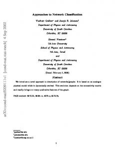
σ = smoothing parameter . The similarity between samples is expressed by the 2 quadratic Euclidean distance k~x −~x ji k2 . The Gaussian function is typically used based on experience and due to its easy implementation. Smoothing parameter σ is used for control of decision regions. Large σ values result in continuous, shallow, rolling regions with σ → ∞ leading to a hyperplane, smaller values cause jagged regions with σ → 0 leading to a nearest neighbor classifier. Figure 1 illustrates this effect. Hence, σ has impact on the generality of decision boundaries. For further discussion of PNN and Parzen windows see e.g. [6, 7, 11, 12, 29, 32]

(a) small σ

(b) large σ

Fig. 1: Different values of σ leading to different activities and decision regions Since we are not interested in the absolute density values but only in their proportions, the simplified function fi (~x) =

1 ni

ni

∑ e−φ /σ

j=1

2

2

with φ = φE2 = k~x −~x ji k2 (2)

can be used with equal σ for all classes instead of the traditional function (1). A non-exponential alternative for saving computation time is calculating 1+1 φ instead

of e−φ /σ in (2). Illustrative interpretation of the density estimator as neural net helps in understanding and enforces acceptance of users. The Parzen estimator PNN is a supervised feedforward neural net consisting of four layers. The input layer is build of one neuron per input variable. Each normalized sample is represented by a weight vector from all input neurons to one hidden neuron in the next pattern layer. A weight vector represents the center of a Parzen window. In the next layer a neuron for each class summarizes all outputs of the hidden neurons – i.e. the results of their exponential activity function – being assigned to one class. The result is a class specific probability density estimation. Output neurons indicate the resulting class. Since each learning sample is represented by a neuron of the pattern 2

layer, each sample is presented once in a one-passlearning approach. Therefore, the size of the pattern layer is determined by the number of samples. Beside of choice of input variables, the only degree of freedom is the value of σ which can easily be modified without relearning. III. Evolutionary Neural Classifiers A. Genetic Learning Vector Quantization and Genetic Probabilistic Neural Net Genetic algorithms (GA), a subgroup of evolutionary algorithms are meta-heuristics imitating the longterm optimization process of biological evolution for solving mathematical optimization problems based upon Darwin’s ’survival of the fittest’. Problem solutions are abstract ’individuals’ in a population. Each solution is evaluated by a fitness function. The fitness value expresses survivability of a solution, i.e. the probability of being a member of the next population and generating ’children’ with similar characteristics by handing down genetic information via evolutionary mechanisms like reproduction, variation and selection, respectively. Genotypes are varied not only by mutation of genes within a single chromosome but also by crossing over, combining characteristics of two solutions in order to get two new solutions. In conjunction with neural nets, GAs can be used for optimization of a net’s weight matrix, the topology or the net parameters, or for determination of the most reasonable input data. The coding of the problem into a genetic representation, e.g. the sequence of the phenotype’s parameters on a genotype, is crucial to the performance of the GA (see e.g. [33– 35] for an overview and more detailed criteria for efficient promising GA approaches, e.g. completeness, compactness and short schemata). The GA-based development of ANNs is an iterative process. A net is constructed by transferring the genotype’s genetic code into a phenotype, i.e. a neural net. After learning (and cross-validation if appropriate), a net is evaluated by a fitness function. Based on this quality information, genetic operations build a new population of nets, which are trained, tested and evaluated again. Thus, the entire learning process can be seen as subdivided into a microscopic cycle of net’s learning and a macroscopic evolutionary one. The iterative learning process of ANNs itself is a part of the entire development process for ANNs, starting from problem modelling and ending at application and maintenance of a net [36]. Combinations of GAs and LVQ can be found e.g. as G-LVQ in [37] or as LVQ-GA in [38]. G-LVQ aims at an improvement of number and initial position of hidden neurons for optimizing classification accuracy, net’s size and data representation separately. LVQ-GA uses a binary gene representation for input data selection, and

an integer coding for determination of the number and initial positions of hidden neurons. We develop a new GA-LVQ, similar to LVQ-GA, and a new GA-PNN. Within genotypes, those net parameters are encoded that have to be genetically varied in order to get net variations. For GA-LVQ and GA-PNN, the importance or influence of input variables is encoded by decimal values controlling ’activity’ of input neurons. They affect the algorithm’s central measure of distance between weight vectors and input vectors by weighting components of the Euclidean distance. Furthermore, for GA-PNN the σ -parameter is part of the genotype. A PNN has a fixed number of hidden neurons determined by the number of learning samples, whereas LVQ’s number of hidden neurons can be varied. For GA-LVQ this number is coded directly. The initial positions of hidden neurons nearby or equal to learning patterns are encoded by a random seed with influence on initialization process. Finer parameters of LVQ, e.g. number of learning iterations, learning rate or window width, can be encoded principally, but are not used in our experiments. The number of output neurons is externally determined by the number of classes. A binary encoding of input neurons allows only binary decisions, whether an input value is used for classification – the input neuron is active – or not. The decimal encoding includes and refines the rough binary coding. It allows graduation, implemented by weighting the values of an input feature for calculating the distance, the crucial factor for the results of distance based classifiers. For each input neuron i a decimal weight ψi with 0 ≤ ψi ≤ 1 is encoded on a gene. A rough graduation seems to be sufficient, e.g. ψi ∈ {0; 0.25; 0.5; 0.75; 1}, ψi ∈ {0; 0.1; . . . ; 0.9; 1} or even finer. With ψi ∈ {0; 1}, the decimal coding is equivalent to binary coding. This relevance weight ψi is used in calculation q of a modified weighted L2 ψ ψ norm k.k2 k~xk2 = + ∑Ni=1 xi2 ψi . The typically used Euclidean distance φE is substituted by a weighted Euclidean distance φψ between two vectors ~a and ~b using these relevance weights: s ψ φψ (~a,~b) = k~a −~bk2 = +

N

∑ (ai − bi )2 ψi .

i=1

φψ = φE is valid for ψi = 1. The ψ -weighting of feature i influences the feature’s impact on the distance by shortening its distance component more (with low factor ψi ) or less (with high factor ψi ). Genetic operators are one- or two-point-crossover and mutation. Crossover is only applied to the chromosome that encodes the input neurons in order to get only genotypes that lead to valid, applicable phenotypes. Furthermore, this gene section can also be varied by mutation of a single gene, inversion of a gene sequence or exchange of two genes. Those genes, that encode the number of hidden neurons and the initialization

parameter, or the value of σ respectively, are varied by mutation only, i.e. adding or subtracting a value within a valid range. A high rate for crossover and a low rate for mutation are recommended. A destabilization is implemented for support of automatization. It interrupts an optimum search being too local and makes the GA more flexible. Here, destabilization means death of accidentally selected individuals and replacement with accidentally constructed new ones. It occurs if a critical fraction of identical or similar individuals exists within a population. The number of individuals to be taken into the new population can be controlled by a rate of survival. A rate of null is equivalent to a restart of an experiment. B. Fitness Function The fitness function is the crucial factor for evaluation and evolution of neural nets providing satisfactory and stable results in real-world applications. A fitness function should favor ANNs with satisfactory generalization ability without using generalization data in order to select useful nets systematically instead of accidentally. Furthermore, the fitness function should represent the user’s objective. In conjunction with ANNs, it allows for evaluation and control of the superordinated evolutionary learning process, thus enhancing the goals nets’ algorithms are aiming at. The mean classification rate (MCR) may be sufficient for some classification tasks. Taking misclassification costs into account seems to be more versatile and also realistic (see e.g. [39] with application of asymmetric costs for time series prediction). A fitness function F for three-class-problems can be e.g. one of the following exemplary ones (with n+ y as number of correctly classified pattern of class y, my as number of all patterns belonging to class y and CRy = n+ y /my ), applied to a learning subset (or better a hold-out subset) of data: F = MCR = (CR1 +CR2 +CR3 )/3 √ F = CR1 ·CR3 or . . . √ F = CR1 ·CR2 ·CR3 or 3 . . . √ F = MCR learn · MCR validation or . . .

(3) (4) (5) (6)

Fitness function (4) aims at uniform high classification rates for classes 1 and 3, whereas fitness (5) favors consistent classification rates for all three classes. Functions aiming at even results on two different subsets of data can be constructed too, see e.g. fitness (6). Besides these direct performance measures in terms of classification rates, a fitness function can include costs for net complexity, e.g. expressed as number of input variables and/or hidden neurons [38]. In general, less complexity leads to better generalization. Thus, the formulation of an appropriate fitness function highly depends on the specific problem to be solved.

Capability of the nets and the fitness function can be evaluated graphically. Results are sorted in descending order of the fitness value (in case of maximizing fitness). The separate charting of fitness values or classification rates for learning, validation and generalization data sets in a two-dimensional scatter diagram allows for evaluation of correlation between the fitness used to control the evolutionary process and the fitness for unknown ’real’ data. Ideally, all results are rudimentary proportional (see s-curve in Fig. 2(a)). A net with high fitness value also yields a satisfactory result for unknown data. Hence, it can be reasonably selected for real application. Fig. 2(b) shows the contrast: deriving a good generalization result from a high fitness is impossible. Nets with good results in application are not preferred systematically within the evolutionary process. A selected net is more or less arbitrarily good or poor. fitness (e.g. average classification rate)

fitness (e.g. average classification rate)

validation data generalization data

validation data generalization data

rank

(a) ideal distributions

rank

(b) poor generalization and/or improper fitness function

Fig. 2: Validation and corresponding generalization The simplest criterion for selection of parents is the fitness value of a single net. Alternatively, a group of some LVQs differing in their initialization value only can be considered in order to make evaluation more independent from the LVQ’s initialization. The group’s fitness can be calculated as arithmetic mean of the single values of each LVQ. For a focus more on the impact of a certain initialization value, only the best fitness within a group can be used as selection criterion. Time consuming computations for different initializations can be supported well by parallel implementation of the algorithms (see next Sect. III-C). The selection itself is implemented as the multi-purpose tournament selection. For details of GA-LVQ, GA-PNN and the complete ANN model building process see [36, 40]. C. Parallelized Implementation A higher computational performance, i.e. a higher number of calculated nets per time unit, can be achieved by parallelization, providing more results. This allows for a more valid evaluation and analysis of the algorithms’ quality. Combinations of data sets and/or individuals of a population can be calculated simultaneously, with variations of initialization for LVQs being coded in a LVQ’s genotype. The nets can be computed in a scalable PC network with one server administrating the population and the genetic algorithm, and

LVQ/PNN-clients getting instructions from the server for computing neural nets and delivering the fitness value. We implement our algorithms of server and client for parallelized GA-LVQ and GA-PNN in C and Visual Basic. At the moment, GA-LVQ supports LVQ1 and LVQ2.1. Verifying experiments succeed: GA-LVQ and GA-PNN are applied to the iris dataset with additional useless input variables, that are correctly recognized and eliminated by ψ -weights = 0. IV. Empirical Evaluation – Real-world Scenario A. Evaluation of Retail Stores For the evaluation of a location of an existing store in terms of sales volume or of an eligible location of a newly planned store, a more or less rough classification of expected sales volume is sufficient [36]. Therefore, estimating the sales volume is a classification problem. Results of a classification process should be used as completion of knowledge of human experts, e.g. for building a priority list for locations to be inspected in detail, not as substitution for invaluable human skills. The data pool consists of external macroscopic up-todate data describing socio-demographic, economical infrastructure at a specific location, e.g. number of homes and residents, retail turnover for different branches of trade, discretionary buying power of a region or number and type of retailers, as well as internal microscopic data describing economical and technical figures of existing stores, e.g. kind of assortment, configuration/equipment components, year of last redecoration, sales volumes for different periods, or sales area. A total of 26 input variables is given. We are interested in sales volumes of a specific product line. They are partitioned in three classes corresponding to possible decisions concerning location policy: • high: establish new store/continue business, • medium: analyze location more detailed, e.g. assortment or in-store design, • low: do not establish new store/shut down store. The task is to classify locations and stores, that are described in numerical patterns. Furthermore, interpretation of classification results should lead to decisions on assortment and in-store design for upgrading a store. B. Computational Experiment Data are pre-partitioned for large, medium and small cities. Class memberships differ for each type of city, because decision rules and definitions of ’high’, ’medium’ or ’low’ sales volumes differ. For each class approximately the same number of examples is available. Disjoint data sets are randomly selected from entire data for learning (roughly 40-70 % of available records), validation (5-25 %) and out-of-sample generalization tests (the rest). Different constellations are used for several experiments in order to get generalized

results for estimation of the methods’ performance. For example, 1 250 data records are available for large cities. They are separated in 940 (840, 740) records forming the learning set, 220 (270, 320) forming the validation set and 90 (140, 190) forming the generalization set. Standard PNN, standard LVQ and basic extensions (e.g. conscience or turned off repulsion in the early learning phase) are computed as implemented within the commercial software NeuralWorks Professional II/Plus with a single PC providing benchmark results. PNN is tested with the hold-one-out method on learning and validation data sets with variations of σ in [0.025, 0.05, . . . , 0.95]. Each LVQ is initialized with 4 different random seeds leading to alternative reproducible starting positions of CVs. The number of CVs is approximately set to 5%, 10%, . . . 25% of the number of learning examples. A standard early stopping rule with variation of its parameters is used in order to avoid overfitting from learning data. Alternatively, variations in fixed numbers of iterations (10/100/500 times the size of the learning set) are analyzed. All 26 input variables are used. Learning schedules, i.e. sequences of Kohonen’s standard algorithms, scaling of input variables and other parameters are taken with standard adjustments recommended in the documentation of NeuralWorks or pre-set by the program. In case of GA-LVQ and GA-PNN, computational experiments are performed on a Pentium-PC-network with one server and up to 60 clients. Various fitness functions based on classification rates are applied to validation data. Variants with binary genetic codes for active/inactive input neurons and decimal codes for gradual activity and resulting weighted input values are tested. For LVQ, early stopping, fixed numbers of iterations are evaluated as well as proportional complexity costs. A population size of 200 is chosen, derived from results of pre-tests. An elitist selection, that always carries over the best net into the next population, is used. C. Results The results of GA-LVQ dominate the results of manually adjusted LVQs, GA-PNN dominates standard PNN. GA-LVQ and GA-PNN provide results on the same level without clear dominance of one approach. The same can be noticed for PNN and LVQ. While results of GA-PNN are slightly higher than results of GA-PNN, GA-LVQ provides results with a little lower variance. Within of GA-LVQ and GA-PNN, results show no favorite fitness function. All classification rates, especially the MCR on generalization data, are in the same satisfying order of magnitude for all three types of city (see Table I, showing results from those nets that are selected for generalization tests due to their promising results on learning and validation data.). Results of the top 10 % of the nets (in respect of MCR on validation

Table I: MCR for generalization data (min/max, group of ’best’ nets); c: conscience, nr: no repulsion Type of city Small Medium Large MCR[%] min max min max min max LVQ c & LVQ1 & LVQ2 LVQ c & nr & LVQ2 GA-LVQ PNN (best σ in [0.25 . . . 0.4]) GA-PNN

57.7 58.4 68.6 60.2 66.4

71.1 71.6 69.7 68.2 71.2

50.1 50.1 69.9 63.6 67.2

60.7 64.1 71.7 67.3 71.8

54.2 57.2 70.0 63.3 68.7

58.8 59.4 71.8 68.9 72.2

of inputs, use of Euclidean distance and only one hidden neuron per class. Some typical properties of a store are given as ’format’, ’type’, ’especially equipped’ and ’duration’. Exemplified weights for analysis of are presented in Table II. Results show strong influence of Table II: LVQ weights, three CVs for three classes (cut-out of exemplified data, scaled [−1; 1]) Property

data) show only a slight higher minimum MCR on generalization data for the manually adjusted nets (up to seven basis points). Even those results are not in the range of the results of GA-LVQ and GA-PNN. As expected, the fitness charts of GA-LVQ and GAPNN show a mixture between Fig. 2(a) and Fig. 2(b) for hold-out data rather than a perfect shaped s-curve. The fitness slightly decreases and the variance from high to low rank increases. On the other hand, charts of classification rates of conventionally developed nets clearly tend to be similar to Fig. 2(b) showing an almost horizontal scatter plot for generalization data. Thus, classification rates on validation data give less or no information about the quality of the nets. Therefore, a systematic selection of a net that generalizes well and reliably is impossible. For GA-LVQ, between 7 and 16, for GA-PNN between 6 and 14 input variables are weighted with 0, the half of the rest is weighted with 0.5. Finer codings have no observable impact on results. For GA-LVQ, the number of hidden neurons depends on the number of used variables. It is in the wide range from 30 to 108. Using the non-zero-weighted inputs as full inputs for NeuralWorks shows inferior or similar results, but no improvement at all. D. Analysis and Interpretation A classification result supports a decision on a location directly. Furthermore, it allows answering the following interesting questions: • What are the main properties of a store making it a member of a special class? Which decisions on in-store design influence sales volume? • Which properties of a location have impact on a store’s class of sales volume? • Which potential for development does a store have? How can this potential be used advantageously? The basic idea with distance based classifiers is the interpretation of CVs and distances between them and input patterns. Those weights wi j from input neuron i to hidden neuron j that have similar values for all hidden neurons lead only to small distance differences. Therefore, the corresponding input features have no or only a weak impact on the classification result. The idea is exemplified assuming evenly relevant weights

Type Special equipment Format A Format B Format C Duration

Class 1 wi1

Class 2 wi2

Class 3 wi3

Weight span

0.65 0.41 −0.97 −0.68 −0.74 −0.32

0.10 0.25 −0.81 −0.88 −0.71 −0.09

−0.42 −0.67 −0.63 −0.98 −0.85 0.07

1.07 1.08 0.34 0.30 0.14 0.39

’type’. A store with a type coded as 1 will be rather classified belonging to class 1 with high sales volume, a type 0 (scaled to −1) to class 3 with low sales volume. ’Special equipment’ or a short ’duration’ – the time period from opening or redecoration – seems to stimulate sales. The ’format’ has less influence. Answers for above mentioned questions can be derived from similar considerations and what-if-analyses by variation of certain values and computing distances for classification. These analyses and interpretations are not bound to usage of the proposed evolutionary net versions. The main results are feasible since they meet with approval of human experts involved in the topic of retail stores and evaluation of locations. V. Conclusions The proposed GA-LVQ and GA-PNN show promising results for decision support in a complex economic real-world classification problem. The results dominate results of conventionally applied standard LVQ and PNN. A fitness function allows control in respect of decision maker’s goal beyond the potential of the nets’ algorithms. For LVQ, common problems like reasonable initialization and values for learning parameters remain. They are mitigated by an evolutionary development with computation of a high number of nets in a parallel PC network implementation. Within the model building process, decisions on ANN’s topology are automated. On the one hand the degrees of freedom concerning parameters of neural learning are reduced, on the other hand new ones concerning evolutionary learning arise. Results may be improved by enhancements of the proposed methods, e.g. application of more ANNs in a committee with each net voting for a class –influence of different voting rules can be studied, combination of different classification methods like support vector machines or distance-based rejection of classification. Furthermore, the influence of different fitness functions on results is an interesting research topic. An important

information for decision makers is the significance of results. The interpretation of the distances between CVs and the object to be evaluated may provide this information. Further research should focus on comparison between GA-LVQ, GA-PNN and several newer LVQ enhancements like LVQ4 or on implementation of those newer LVQ algorithms into GA-LVQ. Moreover, GALVQ and GA-PNN should be applied to other realworld classification problems striving for a broader overlook and better evaluation of the methods’ overall performance. References [1] C. M. Bishop, Neural Networks for Pattern Recognition. Oxford: Clarendon Press, 1995. [2] C. J. C. Burges, “A tutorial on support vector machines for pattern recognition,” Data Mining and Knowledge Discovery, vol. 2 (2), pp. 121–167, 1998. [3] S. S. Haykin, Neural networks : a comprehensive foundation, 2nd ed. Upper Saddle River, NJ: Prentice Hall, 1999. [4] J. Shawe-Taylor and N. Cristianini, Kernel Methods for Pattern Analysis. Cambridge: Cambridge University Press, 2004. [5] T. Kohonen, Self-Organizing Maps, 2nd ed. Berlin: Springer, 1997, vol. 30. [6] L. Fausett, Fundamentals of Neural Networks : architectures, algorithms, and applications. Englewood Cliffs, NJ: PrenticeHall, 1994. [7] D. W. Patterson, Artificial neural networks: theory and applications. Singapore: Prentice Hall, 1996. [8] N. Kitajima, “A New Method for Initializing Reference Vectors in LVQ,” in Proc. ICNN ’95, Proc. of IEEE Intern. Conf. on Neural Networks (Perth, Australia), IEEE, Ed., vol. 5. IEEE Service Center, 1995, pp. 2775–2779. [9] J. T. Laaksonen, “A method for analyzing decision regions in Learning Vector Quantization algorithms,” in Artificial Neural Networks, 2 – Proc. Intern. Conf. on Artificial Neural Networks ICANN-92 (Brighton, GB), I. Aleksander and J. Taylor, Eds., vol. 2. Amsterdam: Elsevier, 1992, pp. 1181–1184. [10] T. Y. Young and T. W. Calvert, Classification, Estimation and Pattern Recognition. New York: American Elsevier, 1974. [11] J. Schürmann, Pattern classification: a unified view of statistical and neural approaches. New York: Wiley & Sons, 1996. [12] R. O. Duda, P. E. Hart, and D. G. Stork, Pattern Classification, 2nd ed. New York: Wiley & Sons, 2001. [13] T. Hastie, R. Tibshirani, and J. Friedman, The Elements of Statistical Learning : Data Mining, Inference, and Prediction. New York: Springer, 2001. [14] D. DeSieno, “Adding a Conscience to Competitive Learning,” in Proc. ICNN ’88, Proc. of IEEE Intern. Conf. on Neural Networks, IEEE, Ed., vol. I. Piscataway, NJ: IEEE Service Center, 1988, pp. 117–124. [15] NeuralWare, Inc., Neural Computing : A Technology Handbook for Professional II/Plus and NeuralWorks Explorer, NeuralWare, Inc., Technical Publications Group, Pittsburgh, PA, 1993. [16] N. R. Pal, J. C. Bedzek, and E. C.-K. Taso, “Generalized Clustering Networks and Kohonen’s Self-Organizing Scheme,” in IEEE Transactions on Neural Networks, vol. 3 (4). IEEE, 1993, pp. 546–557. [17] M. Verleysen, P. Thissen, and J.-D. Legat, “Linear vector classification: An improvement on LVQ algorithms to create classes of patterns,” in New Trends in Neural Computation – Proc. Intern. Workshop on ANN (IWANN ’93), Sitges, Spain, June 1993, J. Mira, J. Cabestany, and A. Prieto, Eds. Berlin: Springer, 1993, pp. 340–345. [18] M. Pregenzer, D. Flotzinger, and G. Pfurtscheller, “Distinction Sensitive Learning Vector Quantisation – a new noise-insensitive classification method,” in Proc. ICNN ’94, Proc. of IEEE Intern. Conf. on Neural Networks (Orlando, FL), IEEE, Ed., vol. V. Piscataway, NJ: IEEE Service Center, 1994, pp. 2890–2894.

[19] A. Zell, Simulation Neuronaler Netze. Bonn: Addison-Wesley, 1994. [20] S.-J. You and C.-H. Choi, “LVQ with a Weighted Objective Function,” in Proc. ICNN ’95, Proc. of IEEE Intern. Conf. on Neural Networks (Perth, Australia), IEEE, Ed., vol. 5. IEEE Service Center, 1995, pp. 2763–2768. [21] R. Odorico, “Learning Vector Quantization with Training Count (LVQTC),” Neural Networks, vol. 10 (6), pp. 1083–1088, 1997. [22] A. Sato, “An Analysis of Initial State Dependence in Generalized LVQ,” in Ninth Intern. Conf. on Artificial Neural Networks (ICANN 99) – (Conf. Publ. No. 470), vol. 2, 1999, pp. 928–933. [23] B. Hammer, M. Strickert, and T. Villmann, “Learning Vector Quantization for Multimodal Data,” in Artificial Neural Networks - Proc. of ICANN 2002 : Intern. Conf., Madrid, Spain, Aug 28-30, 2002. Heidelberg: Springer, 2002, pp. 370–376. [24] S. Seo and K. Obermayer, “Soft Learning Vector Quantization,” Neural Computation, vol. 15, pp. 1589–1604, 2003. [25] M.-T. Vakil-Baghmisheh and N. Pavesic, “Premature clustering phenomenon and new training algorithms for LVQ,” Pattern Recognition, vol. 36 (8), pp. 1901–1912, 2003. [26] D. F. Specht, “Probabilistic Neural Networks for Classification, Mapping or Associative Memory,” in Proc. ICNN ’88, Proc. of IEEE Intern. Conf. on Neural Networks, IEEE, Ed., vol. 1. Piscataway, NJ: IEEE Service Center, 1988, pp. 525–532. [27] ——, “Probabilistic neural networks and the polynomial Adaline as complementary techniques for classification,” in Transactions on Neural Networks, IEEE, Ed., vol. 1 (1). New York, NY: IEEE Neural Networks Council, 1990, pp. 111–121. [28] ——, “Probabilistic neural networks,” Neural Networks, vol. 3, pp. 109–118, 1990. [29] E. Parzen, “On estimation of a probability density function and mode,” Annals of Mathematical Statistics, vol. 33, pp. 1065– 1076, 1962. [30] T. Cacoullos, “Estimation of a multivariate density,” Annals of the Institute of Statistical Mathematics (Tokyo), vol. 18 (2), pp. 179–189, 1962. [31] V. N. Vapnik, The Nature of Statistical Learning Theory. New York: Springer, 1995. [32] C. Jutten and P. Comon, “Neural Bayesian Classifier,” in New Trends in Neural Computation – Proc. Intern. Workshop on ANN (IWANN ’93), Sitges, Spain, June 1993, J. Mira, J. Cabestany, and A. Prieto, Eds. Berlin: Springer, 1993, pp. 119–124. [33] D. E. Goldberg, Genetic Algorithms in Search, Optimization, and Machine Learning. Reading, MA: Addison-Wesley, 1989. [34] J. H. Holland, Adaptation in natural and artificial systems : an introductory analysis with applications to biology, control, and artificial intelligence. Cambridge, MA: MIT Press, 1994. [35] Z. Michalewicz, Genetic Algorithms + Data Structures = Evolution Programs, 2nd ed. Berlin: Springer, 1994. [36] R. Stahlbock, Evolutionäre Entwicklung künstlicher neuronaler Netze zur Lösung betriebswirtschaftlicher Klassifikationsprobleme. Berlin: WiKu, 2002. [37] J. Merelo and A. Prieto, “G-LVQ, a combination of genetic algorithms and LVQ,” in Artificial Neural Nets and Genetic Algorithms – Proc. Intern. Conf. 1995 (Alès, Frankreich), D. W. Pearson, N. C. Steele, and R. F. Albrecht, Eds. Wien: Springer, 1995, pp. 92–95. [38] U. Derigs and G. Schirp, “Genetische Modellierung von Künstlichen Neuronalen Netzen : Erfahrungen beim Einsatz zur Kreditwürdigkeitsprüfung,” OR Spektrum, no. 19, pp. 285–293, 1997. [39] S. F. Crone, “Training Artificial Neural Networks using Asymmetric Cost Functions,” in Proc. 9th Int. Conf. on Neural Information Processing (ICONIP’02) – Computational Intelligence for the E-Age, Nov 18-22, 2002, Singapore, L. Wang, C. Rajapakse, K. Fukushima, S.-Y. Lee, and X. Yao, Eds., vol. 5. Piscataway, NJ: IEEE Service Center, 2002, pp. 2374–2380. [40] R. Stahlbock, “An evolutionary neural classification approach to evaluate retail stores and support decisions on their location, in-store design and assortment,” in Proc. of the Int. Conf. on Artificial Intelligence (IC-AI’04), Las Vegas, Nevada, USA, June 21–24, H. Arabnia, Ed., vol. I. CSREA Press, 2004, pp. 228– 234.