McKay 1982), and focused reasoning (Schlegel and Shapiro. 2014a) ..... proaches include a tree-based approach called a P-Tree, a .... ment of Dr. John Lavery.
Cedex France [email protected] ...... M. d'Amico, P. Frosini, C. Landi, Optimal Matching between Reduced Size Func- tions, Tech. Report 35 ...
via Bayes Theorem from a prior on the space of distribution functions. The fact ... empirical distribution function Fn of X1,..., Xn. In particular, for every Borel.
Mar 30, 2009 - ibara et al., 2006) and Saint-Malo (Clark et al.,. 2008). In the proceedings of .... Alexander Clark, Remi Eyraud and Amaury. Habrard (A note on ...
Apr 4, 2012 - KEY WORDS: Phylodynamics, Viral evolution, Experimental design, Phylogenetic ... 2012) as well as bacterial pathogens (Harris et al.,. 2010 ...
Section 5 and 6 describe BUNDLE and TRILL .... L(ãa, bã); 3) Merge(a, b), the merging of the nodes a, b; 4) =(a, b), the ..... Call to Pellet. 9: ..... IOS Press (2008).
May 6, 2011 - We design a MapReduce performance model, that for a given job (with a ...... Twitter application counts the number of asymmetric links in the ...
acquisition tools to operate as a server on the World Wide Web, allowing a web client .... When the knowledge selects a factored EDAG in the control panel at the ...
The Logic of Interpreting Evidence of Developmental Ordering: Strong Inference and Categorical Measures. James A. Dixon. College of William and Mary.
being taken by corporate networks and business cus- ..... finding contact and registration information for In- ..... of inferred siblings are confirmed by AT&T. These.
May 6, 2011 - MapReduce and Hadoop represent an economically com- pelling alternative for efficient large scale data processing and advanced analytics in ...
Dec 9, 2009 - group behavior gives SocialFusion the best opportunity ... move, the mobile application passes on fresh values at ...... expression builder.
Nov 1, 2013 - Abstract: This paper describes the Bayesian inference and prediction of the generalized Pareto (GP) distribution for progressive first-.
In the realm of software engineering, context-free grammars (CFGs) are of paramount ... This enables a domain expert to create a DSL by supplying sentences.
domain knowledge; information inference; short text; text categorization; ... web short texts are derived from a variety of domains, and possess real-time ...
BLOG is a powerful language to express models with an un- known number of objects and identity uncertainty. Current inference engines for BLOG are either ...
Oct 14, 2015 - (2) another, unobserved neuron C affects both A and B. To deal with this issue, ..... This direct approach is simple and computationally quite cheap. ..... 2 а 106 time bins), a similar simulation on a standard laptop (Fig 5) takes.
May 12, 2011 - Indian Statistical Institute. Kolkata, India ... Trademark Notice: Product or corporate names may be trademarks or registered trademarks, and are.
Apr 14, 2009 - Buard J, de Massy B (2007) Playing hide and seek with mammalian meiotic crossover hotspots. Trends Genet 23:301â309. 7. Stumpf M ...
A pleasant corollary from this invariance structure, which follows from the fact that the group .... Corollary 3.1. ...... 50, Avenue F.D. Roosevelt, CP114/04. B-1050 ...
Sep 25, 2014 - Frank and Nowak, 2004; Biesecker and Spinner, 2013; Frank and Nowak, 2003; De ... Bedard et al., 2013; Navin et al., 2011; Ding et al., 2012).
duction/abduction/induction triad is defined formally in terms of the position of the ... the terminology introduced by
tages of a Bayesian analysis. From a theoretical perspective, Bayesian inference is principled and prescriptive, and â in contrast to frequentist inference â a ...
May 10, 2017 - Ecology and Evolution published by John Wiley & Sons Ltd. ... i'th dimension in the p- dimensional habitat space), and c[ = exp (β0), where β0 is the ... ately termed a âresource unitâ (Lele, Merrill, Keim, & Boyce, 2013). The.
|
|
Received: 14 March 2017 Revised: 12 April 2017 Accepted: 10 May 2017 DOI: 10.1002/ece3.3122
ORIGINAL RESEARCH
Relative Selection Strength: Quantifying effect size in habitat-and step-selection inference Tal Avgar1
| Subhash R. Lele2 | Jonah L. Keim3 | Mark S. Boyce1
1 Department of Biological Sciences, University of Alberta, Edmonton, AB, Canada 2 Department of Mathematical and Statistical Sciences, University of Alberta, Edmonton, AB, Canada 3 Trove Predictive Data Science, Edmonton, AB, Canada
Correspondence Tal Avgar, Department of Integrative Biology, University of Guelph, Guelph, ON, Canada. Email: [email protected] Funding information Banting Postdoctoral Fellowship for TA
Abstract Habitat-selection analysis lacks an appropriate measure of the ecological significance of the statistical estimates—a practical interpretation of the magnitude of the selection coefficients. There is a need for a standard approach that allows relating the strength of selection to a change in habitat conditions across space, a quantification of the estimated effect size that can be compared both within and across studies. We offer a solution, based on the epidemiological risk ratio, which we term the relative selection strength (RSS). For a “used-available” design with an exponential selection function, the RSS provides an appropriate interpretation of the magnitude of the estimated selection coefficients, conditional on all other covariates being fixed. This is similar to the interpretation of the regression coefficients in any multivariable regression analysis. Although technically correct, the conditional interpretation may be inappropriate when attempting to predict habitat use across a given landscape. Hence, we also provide a simple graphical tool that communicates both the conditional and average effect of the change in one covariate. The average-effect plot answers the question: What is the average change in the space use probability as we change the covariate of interest, while averaging over possible values of other covariates? We illustrate an application of the average-effect plot for the average effect of distance to road on space use for elk (Cervus elaphus) during the hunting season. We provide a list of potentially useful RSS expressions and discuss the utility of the RSS in the context of common ecological applications. KEYWORDS
& Avgar, 2017a). Estimation of the parameters in the HSA under
1984). Of course, habitat components can be a mixture of discrete and
the local-availability assumption (e.g., SSA/iSSA) is carried out using
continuous variables, and hence, the joint normal distribution assump-
conditional logistic regression (case–control design), where each
tion for such a collection may be violated in many studies. Arguments
used location is coupled with, and contrasted against, a conditional
have been made against the use of the exponential form for the RSPF
availability set, sampled based on proximity in space and/or time.
due to the unreasonable parameter bounding it requires (Lele, 2009;
These models are, thus, computationally easy to fit. Whether one
Lele & Keim, 2006; McDonald, 2013).
uses static availability (e.g., study area wide with no temporal de-
The exponential form is nevertheless by far the most commonly
pendencies) or dynamic availability (e.g., availability is defined by a
used functional form in HSA. The majority of habitat-selection stud-
movement kernel centered on the previously observed position), the
ies are based on survey or telemetry approaches which inform us
basic HSA still relies on a used-available design and an exponential
where animals are, but not necessarily where they are not, resulting
selection function.
in a “used-available” (rather than a “used–unused”) design (Manly et al., 2002; McDonald, 2013). The prevalence of used-available design is likely a key reason for the popularity of the exponential HSA, because under this design, the selection coefficients (i.e., the βi’s in Equation 1) can be estimated using logistic regression, making
2 | INTERPRETATION OF EXPONENTIAL HSA AND THE β COEFFICIENTS
it highly accessible (Johnson, Nielsen, Merrill, McDonald, & Boyce,
Used-available (whether static or dynamic) exponential HSAs allow
2006; McDonald, 2013). Under the used-available design, however,
the estimation of what is known in epidemiology as the “relative risk”
the normalizing constant, c, in the exponential model, is nonidenti-
or “risk ratio” (Miettinen, 1972). Relative risk is the ratio of the prob-
fiable (Lele & Keim, 2006), and hence, inference can be drawn only
ability of an event occurring in a treatment group to the probability of
about the relative probability of selection, resulting in an RSF rather
the event occurring in a control group. Because we are working in the
than an RSPF. Note that considering the HSA results as yielding rel-
context of habitat selection, we shall refer to it as the relative selec-
ative probability of selection, without mentioning the underlying
tion strength (RSS).
exponential model, is misleading; if the underlying functional form is not of the type described in equation 1, such a blanket statement is incorrect. One of the major, and as yet unresolved, problems in used- available study design is the identification of available resource units, namely which resource units will be considered for use by the individual. A simplistic approach assumes that all resource units in the study area (often an arbitrary definition in itself) are equally
2.1 | Relative selection strength between two spatial locations Let x1 and x2 denote the spatial coordinates of two locations. Then, RSS (x2, x1) = w(x2)/w(x1). Under the exponential model, this can be ) ( simplified as RSS(x2 , x1 ) = exp{Σpi=1 βi hi (x2 ) − hi (x1 ) }. Notice that this only depends on the difference in the habitat conditions between
considered for use if there is no selection. This has been modified
the two locations (or, in the case of an SSA/iSSA, the difference be-
to reflect the fact that not all resource units are equally encounter-
tween two steps sharing the same starting point but ending in x1 and
able. This leads to consideration of local availability that assumes all
x2). Moreover, this does not depend on the normalizing parameter
|
AVGAR et al.
5324
c[ = exp (β0)]. This ratio takes a value between 0 and ∞ and tells us
conditional log-RSS over a unit distance in habitat space. If the two
which location, given that it is encountered, has a relatively higher
locations differ by two habitat components, hi and hj, the condi-
probability of selection and by how much. There is a word of cau-
tional log-RSS is βi∙Δhi + βj∙Δhj, etc. Hence, in these simple cases, the
tion, however. Suppose there are four locations with w(x1) = 0.18, w
conditional RSS is sensitive only to the selection coefficients and the
(x2) = 0.90, w(x3) = 0.001, w(x4) = 0.005 as the selection probabilities.
difference in habitat values (distance in habitat space), but not to the
Then, RSS (x2, x1) = RSS (x4, x3) = 5. The RSS tells us that x2 is 5 times
absolute value of the habitat.
more probable than x1 but so is x4 five times more probable than x3.
• If the HSA includes an interaction between hi and hj (hi·hj), with a
However, we would not treat those relationships to be equally impor-
corresponding selection coefficient βij, and given that hj(x1) = hj(x2),
tant because the change in the first case seems ecologically far more
the conditional log-RSS is given by Δhi ⋅(βi + βij ⋅hj (x1 )] (see Figure 1).
important than in the second case.
• If the HSA includes, in addition to hi, a squared term for hi ⋅(h2i ), with a corresponding selection coefficient βi2, the conditional log-RSS is given by Δhi ⋅(βi + βi2 ⋅[2⋅hi (x1 ) − Δhi ]). Hence, in this case (and all
2.2 | Effect of a habitat covariate on selection
subsequent cases), the log-RSS is sensitive, in addition to the selection
Aside from comparing two locations, in practice, we also want to
coefficients and the distance in habitat space,to the position in habitat
know how the change in one of the habitat covariates will affect the
space (i.e., the habitat value).
probability of selection. This is a classic problem of interpretation
• In the combined case, where both a quadratic term and an in-
of regression coefficients in multiple regression models. For example, we might want to interpret β1, the coefficient corresponding to
teraction are included, the conditional log-RSS is given by ( [ ( ) ] ( )) Δhi ⋅ βi + βi2 ⋅ 2⋅hi x1 − Δhi + βij ⋅hj x1 .
the habitat covariate h1 in equation 1. Suppose we change the value
• In the case where the habitat value is log-transformed [ = ln (hi)],
of h1 by one unit and keep all other habitat covariates the same. is the RSS of habitat covariate h1, provided all other covariates in
with a corresponding selection coefficient βi, the conditional log] [ h x ( 1 ) βi RSS is given by ln h xi −Δh (see Barrera-Gómez & Basagaña ( ) i 1 i 2015 for further discussion of log-transformed variables). Hence,
the model do not change. This is a conditional interpretation that
log-transformed variables mean that the relative selection strength
is not the effect of the covariate h1without any reference to other
is a function of the ratio, rather than the difference, between avail-
covariates. Suppose we fit three different models; one with only h1,
one with two covariates, h1 and h2, and one with three covariates h1,
• In the case where the habitat value is log-transformed, and there
h2, and h3; as in any other multiple regression, the estimated coef-
is an interaction with a second habitat component, hj, with a corre( ) ( ) sponding selection coefficient βij, and given that hj x1 = hj x2 , the ] [ h x ( 1 ) [βi +βij hj (x1 )] conditional log-RSS is given by ln h xi −Δh . i( 1) i • Lastly, in the case where two covariates, hi and hj, are log-trans-
ficient corresponding to h1 in these three models, except in some rare situations, will be different (Seber, 1984). The inferred value of β1 and the interpretation of exp(β1)as the RSS is conditional on what other covariates are included in the model, what their values
formed, the conditional log-RSS for x1 in relation to x2 is given by ]βi [ h x ] [ h x ( 1 ) βj i( 1) + ln h xj −Δh . hi (x1 )−Δhi ( ) j 1 j
are, and whether these covariates are correlated or have correlated
ln
effects. Hence, this interpretation should not be thoughtlessly exported to other studies (but see below for a graphical methods for inference transferability). 20
3 | COMMON RSS EXPRESSIONS In our experience, certain statistical transformations and interactions are particularly common in HSA and SSA formulations. Here, we list the corresponding log-RSS expressions in hope this will facilitate ease of use and interpretation. Note again that these are based on the assumption that all covariates not explicitly mentioned are kept constant. • The log-RSS for location x1 in relation to location x2, given that these two locations share the same values for all habitat covariates but one, hi, is βi∙Δhi, where Δhi = hi(x1) − hi(x2). For (i)SSA, x1 and x2 are further assumed to mark the end points of two steps starting from the same point in space and time (and hence sharing the same availability domain) and equal in their length (and any other attribute of the underlying movement kernel). In other words, βi is the
log RSS for x1versus x2
15 10 5 0 –5
0
100
200
300
400
500
600
Elevation at x1 (m)
700
800
900
1,000
F I G U R E 1 Log-RSS for one spatial position (x1) over another (x2) as function of elevation and habitat type (“meadow” = dashed line; “forest” = dotted line) at x1. The RSF includes two main effects, one ctegorical (“forest”/“meadow”) and one continuous (elevation), as well as their interaction, and is given by exp (1⋅forest + 0.01⋅elevation + 0.01⋅elevation⋅forest). Elevation at x2 is 500 m, and habitat at x2 is “meadow” (the reference category for the RSF)
|
5325
AVGAR et al.
4 | AVERAGE EFFECT OF A HABITAT COVARIATE The conditional interpretation of exp(β1) (i.e., the RSS) may be difficult to use when attempting to predict the intensity of space use as function of a focal covariate across a particular study area or management unit, where other covariates may, or may not, change in conjunction with the focal covariate. What one can, however, study is the average change in the response as we change h1, averaged over all possible values of other covariates in the model. This interpretation still depends on what other covariates are present in the model, but it removes the problem of interpretation in the presence of correlations and conditioning on all other covariates not changing. This idea can be applied even in the case of an RSPF model, where the absolute probability of selection is computed. The mathematical details underlying this idea are presented in the Appendix. Before proceeding further, we discuss the relationship between the RSS and the average effect depicted in the graphical tool. The probability of use is equivalent to the average probability of selection, averaged over all available units (Lele et al., 2013). Such an averaging weighs the probability of selection of a habitat type with the probability of encountering that habitat type. For a given probability of selection, higher encounter rate leads to higher probability of use, and inversely, lower encounter rate leads to lower probability of use (see Keim, DeWitt, & Lele, 2011). The graphical tool we describe here depicts the change in the average probability of selection as we change one of the habitat covariates while averaging over other habitat covariates according to their availability. Because we have averaged the selection probability over available resource units, this depicts the change in the probability of use, and not the change in the probability of selection. As will be illustrated below, if the availability of other resources changes, the graph depicting the probability of use also changes.
5 | VISUALIZING THE AVERAGE EFFECT OF DISTANCE TO ROAD ON ELK SPACE USE
randomly distributed points (available locations) situated within 3 km of off-highway roads. The analysis considers two covariates: habitat suitability index and distance to road (km). The habitat suitability index for any location was calculated based on a separate RSPF model fitted to an independent dataset on elk habitat-use collected in the surrounding area. This RSPF model did not include distance to road as a covariate. The habitat suitability covariate, thus, stands as a proxy for including several habitat covariates such as terrain measures (e.g., slope, elevation, and aspect) and vegetation indices (e.g., normalized difference vegetation index). We used the ResourceSelection package in R to estimate both the exponential RSF and the logistic RSPF models (Lele & Keim, 2006; Sólymos & Lele, 2016) from the data (Table 1 and 2). This package is readily available from CRAN (https://cran.r-project.org/web/packages/ResourceSelection/index.html) and can be applied using standard framework in R, similar to fitting a generalized linear model. Both the exponential and logistic models included an interaction effect between habitat suitability and road distance. We do not intend to discuss the model selection and appropriateness of different models, so only in passing we note that, based on the AIC, the logistic RSPF model had a better fit to the data than the exponential RSF model (AIC difference −415.826).
5.1 | Average effect of distance to road, averaged over all habitat conditions other than the distance to the road To visualize the average effect of distance to road on the probability of space use by elk, we conducted the following analysis. 1. Fit the exponential RSF (or, logistic RSPF) model using two covariates; habitat suitability index and distance to road. 2. Compute the fitted exponential RSF (or, logistic RSPF) values at the available locations, namely {w(x1), w(x2), …, w(xN)}. T A B L E 1 Exponential resource selection function model Parameter
Parameter estimate
SE
Z-Value
Pr(>|Z|)
We offer an example illustrating the graphical method to help visual-