Section 5 and 6 describe BUNDLE and TRILL .... L(ãa, bã); 3) Merge(a, b), the merging of the nodes a, b; 4) =(a, b), the ..... Call to Pellet. 9: ..... IOS Press (2008).
Semantics and Inference for Probabilistic Description Logics Riccardo Zese1 , Elena Bellodi1 , Evelina Lamma1 , Fabrizio Riguzzi2 , and Fabiano Aguiari1 1
Dipartimento di Ingegneria – University of Ferrara Dipartimento di Matematica e Informatica – University of Ferrara Via Saragat 1, I-44122, Ferrara, Italy [riccardo.zese,elena.bellodi,evelina.lamma,fabrizio.riguzzi]@unife.it 2
Abstract. We present a semantics for Probabilistic Description Logics that is based on the distribution semantics for Probabilistic Logic Programming. The semantics, called DISPONTE, allows to express assertional probabilistic statements. We also present two systems for computing the probability of queries to probabilistic knowledge bases: BUNDLE and TRILL. BUNDLE is based on the Pellet reasoner while TRILL exploits the declarative Prolog language. Both algorithms compute a propositional Boolean formula that represents the set of explanations to the query. BUNDLE builds a formula in Disjunctive Normal Form in which each disjunct corresponds to an explanation while TRILL computes a general Boolean pinpointing formula using the techniques proposed by Baader and Pe˜ naloza. Both algorithms then build a Binary Decision Diagram (BDD) representing the formula and compute the probability from the BDD using a dynamic programming algorithm. We also present experiments comparing the performance of BUNDLE and TRILL.
1
Introduction
The main idea of the Semantic Web is making information available in a form that is understandable and automatically manageable by machines [16]. In order to realize this vision, the W3C has supported the development of a family of knowledge representation formalisms of increasing complexity for defining ontologies, called Web Ontology Language (OWL). In particular, OWL defines the sublanguages OWL-Lite, OWL-DL (based on Description Logics) and OWL-Full. Since the real world often contains uncertain information, it is fundamental to be able to represent and reason with such information. This problem has been investigated by various authors both in the general case of First Order Logic (FOL) [27, 14, 5] and in the case of restricted logics, such as Description Logics (DLs) and Logic Programming (LP). In particular, in LP the distribution semantics [39] has emerged as one of the most effective approaches for representing probabilistic information and it underlies many probabilistic LP languages such as Probabilistic Horn Abduction [30], PRISM [39, 40], Independent Choice Logic [29], Logic Programs with Annotated Disjunctions [47], ProbLog [9] and CP-logic [46].
In [7, 34, 37, 36] we applied the distribution semantics to DLs obtaining DISPONTE for “DIstribution Semantics for Probabilistic ONTologiEs” (Spanish for “get ready”), in which we annotate axioms of a theory with a probability and assume that each axiom is independent of the others. A DISPONTE knowledge base (KB for short) defines a probability distribution over regular KBs (worlds) and the probability of a query is obtained from the joint probability of the worlds and the query. In order to fully support the development of the Semantic Web, efficient DL reasoners, such us Pellet [44], RacerPro [12] and HermiT [43], are used to extract implicit information from the modeled ontologies, and probabilistic DL reasoners, such as PRONTO [21], are used to compute the probability of the inferred information. Most DL reasoners implement a tableau algorithm in a procedural language. However, some tableau expansion rules are non-deterministic, requiring the developers to implement a search strategy in an or-branching search space. Moreover, in some cases we want to compute all explanations for a query, thus requiring the exploration of all the non-deterministic choices of the tableau algorithm. We present the algorithm BUNDLE for “Binary decision diagrams for Uncertain reasoNing on Description Logic thEories”, that performs inference over DISPONTE DLs. BUNDLE exploits an underlying reasoner such as Pellet [44] that returns explanations for queries. Moreover, we present the system TRILL for “Tableau Reasoner for descrIption Logics in proLog”, a tableau reasoner implemented in the declarative Prolog language. Prolog’s search strategy is exploited for taking into account the nondeterminism of the tableau rules. TRILL uses the Thea2 library [45] for parsing OWL in its various dialects. Thea2 translates OWL files into a Prolog representation in which each axiom is mapped into a fact. TRILL can check the consistency of a concept and the entailment of an axiom from an ontology, and can return the “pinpointing formula” for queries. Both BUNDLE and TRILL use the inference techniques developed for probabilistic logic programs under the distribution semantics, in particular Binary Decision Diagrams (BDDs), for computing the probability of queries from the set of all explanations and the pinpointing formula respectively. They encode the results of the inference process in a BDD from which the probability can be computed in time linear in the size of the diagram. In the following, Section 2 briefly introduces ALC and SHOIN (D) DLs. Section 3 presents the DISPONTE semantics while Section 4 defines the problem of answering queries to DLs. Section 5 and 6 describe BUNDLE and TRILL respectively. Section 7 illustrates related work. Section 8 shows experiments and Section 9 concludes the paper.
2
Description Logics
Description Logics (DLs) are knowledge representation formalisms that possess nice computational properties such as decidability and/or low complexity, see 2
[1, 2] for excellent introductions. DLs are particularly useful for representing ontologies and have been adopted as the basis of the Semantic Web. While DLs can be translated into FOL, they are usually represented using a syntax based on concepts and roles. A concept corresponds to a set of individuals of the domain while a role corresponds to a set of pairs of individuals of the domain. We first briefly describe ALC and then SHOIN (D), showing the difference with ALC. Let A, R and I be sets of atomic concepts, roles and individuals, respectively. Concepts are defined by induction as follows. Each C ∈ A is a concept, ⊥ and > are concepts. If C, C1 and C2 are concepts and R ∈ R, then (C1 u C2 ), (C1 t C2 ) and ¬C are concepts, as well as ∃R.C and ∀R.C. A TBox T is a finite set of concept inclusion axioms C v D, where C and D are concepts. We use C ≡ D to abbreviate the conjunction of C v D and D v C. An ABox A is a finite set of concept membership axioms a : C, role membership axioms (a, b) : R, equality axioms a = b and inequality axioms a 6= b, where C is a concept, R ∈ R and a, b ∈ I. A knowledge base K = (T , A) consists of a TBox T and an ABox A. A knowledge base K is usually assigned a semantics in terms of interpretations I = (∆I , ·I ), where ∆I is a non-empty domain and ·I is the interpretation function that assigns an element in ∆I to each a ∈ I, a subset of ∆I to each C ∈ A and a subset of ∆I × ∆I to each R ∈ R. The mapping ·I is extended to all concepts (where RI (x) = {y|(x, y) ∈ RI }) as: >I ⊥I (C1 u C2 )I (C1 t C2 )I (¬C)I (∀R.C)I (∃R.C)I
= ∆I =∅ = C1I ∩ C2I = C1I ∪ C2I = ∆I \ C I = {x ∈ ∆I |RI (x) ⊆ C I } = {x ∈ ∆I |RI (x) ∩ C I 6= ∅}
The satisfaction of an axiom E in an interpretation I = (∆I , ·I ), denoted by I |= E, is defined as follows: (1) I |= C v D iff C I ⊆ DI , (2) I |= a : C iff aI ∈ C I , (3) I |= (a, b) : R iff (aI , bI ) ∈ RI , (4) I |= a = b iff aI = bI , (5) I |= a 6= b iff aI 6= bI . I satisfies a set of axioms E, denoted by I |= E, iff I |= E for all E ∈ E. An interpretation I satisfies a knowledge base K = (T , A), denoted I |= K, iff I satisfies T and A. In this case we say that I is a model of K. In following we describe SHOIN (D) showing what it adds to ALC. A role is either an atomic role R ∈ R or the inverse R− of an atomic role R ∈ R. We use R− to denote the set of all inverses of roles in R. An RBox R consists of a finite set of transitivity axioms T rans(R), where R ∈ R, and role inclusion axioms R v S, where R, S ∈ R ∪ R− . If a ∈ I, then {a} is a concept called nominal, and if C, C1 and C2 are concepts and R ∈ R ∪ R− , then ≥ nR and ≤ nR for an integer n ≥ 0 are also 3
concepts. A SHOIN (D) KB K = (T , R, A) consists of a TBox T , an RBox R and an ABox A. The mapping ·I is extended to all new concepts (where #X denotes the cardinality of the set X) as: (R− )I {a}I (≥ nR)I (≤ nR)I
= {(y, x)|(x, y) ∈ RI } = {aI } = {x ∈ ∆I |#RI (x) ≥ n} = {x ∈ ∆I |#RI (x) ≤ n}
SHOIN (D) allows the definition of datatype roles, i.e., roles that map an individual to an element of a datatype such as integers, floats, etc. Then new concept definitions involving datatype roles are added that mirror those involving roles introduced above. We also assume that we have predicates over the datatypes. The satisfaction of an axiom E in an interpretation I = (∆I , ·I ), denoted by I |= E, is defined as for ALC, plus the following ones regarding RBox axioms: (6) I |= T rans(R) iff RI is transitive, (7) I |= R v S iff RI ⊆ S I . An interpretation I satisfies a knowledge base K = (T , R, A), denoted I |= K, iff I satisfies T , R and A. In this case we say that I is a model of K. Each DL is decidable if the problem of checking the satisfiability of a KB is decidable. In particular, SHOIN (D) is decidable iff there are no number restrictions on non-simple roles. A role is non-simple iff it is transitive or it has transitive subroles. A query Q over a KB K is usually an axiom for which we want to test the entailment from the KB, written K |= Q. The entailment test may be reduced to checking the unsatisfiability of a concept in the knowledge base, i.e., the emptiness of the concept. For example, the entailment of the axiom C v D may be tested by checking the unsatisfiability of the concept C u ¬D. Example 1. The following KB is inspired by the ontology people+pets [28]: ∃hasAnimal.P et v N atureLover fluffy : Cat tom : Cat Cat v P et (kevin, fluffy) : hasAnimal (kevin, tom) : hasAnimal It states that individuals that own an animal which is a pet are nature lovers and that kevin owns the animals fluffy and tom. Moreover, fluffy and tom are cats and cats are pets. The query Q = kevin : N atureLover is entailed by the KB.
3
The DISPONTE Semantics
DISPONTE [37] applies the distribution semantics [39] of probabilistic logic programming to DLs. A program following this semantics defines a probability 4
distribution over normal logic programs called worlds. Then the distribution is extended to queries and the probability of a query is obtained by marginalizing the joint distribution of the query and the programs. In DISPONTE, a probabilistic knowledge base K contains a set of probabilistic axioms which take the form p :: E (1) where p is a real number in [0, 1] and E is a DL axiom. The idea of DISPONTE is to associate independent Boolean random variables to the probabilistic axioms. To obtain a world w we decide whether to include each probabilistic axiom or not in w. A world therefore is a non probabilistic KB that can be assigned a semantics in the usual way. A query is entailed by a world if it is true in every model of the world. The probability p can be interpreted as an epistemic probability, i.e., as the degree of our belief in axiom E. For example, a probabilistic concept membership axiom p :: a : C means that we have degree of belief p in C(a). A probabilistic concept inclusion axiom of the form p :: C v D represents the fact that we believe in the truth of C v D with probability p. Formally, an atomic choice is a couple (Ei , k) where Ei is the ith probabilistic axiom and k ∈ {0, 1}. k indicates whether Ei is chosen to be included in a world (k = 1) or not (k = 0). A composite choice κ is a consistent set of atomic choices, i.e., (Ei , k) ∈ κ, (Ei , m) ∈ κ implies k = m (only one decision is Q taken for each Q axiom). The probability of a composite choice κ is P (κ) = (Ei ,1)∈κ pi (Ei ,0)∈κ (1 − pi ), where pi is the probability associated with axiom Ei . A selection σ is a total composite choice, i.e., it contains an atomic choice (Ei , k) for every axiom of the theory. A selection σ identifies a theory wσ called a world in this way: wσ = {Ei |(Ei , 1) ∈ σ}. Let us indicate with SK the set of all selections and with Q WK the set Qof all worlds. The probability of a world wσ is P (wσ ) = P (σ) = (Ei ,1)∈σ pi (Ei ,0)∈σ (1 − pi ). P (wσ ) is P a probability distribution over worlds, i.e., w∈WK P (w) = 1. We can now assign probabilities to queries. Given a world w, the probability of a query Q is defined as P (Q|w) = 1 if w |= Q and 0 otherwise. The probability of a query can be defined by marginalizing the joint probability of the query and the worlds: X X X P (Q) = P (Q, w) = P (Q|w)P (w) = P (w) (2) w∈WK
4
w∈WK
w∈WK :w|=Q
Querying KBs
In order to answer queries to DL KBs, a tableau algorithm [42] can be used. Such an algorithm decides whether an axiom is entailed or not by a KB by refutation: axiom E is entailed if ¬E has no model in the KB. The algorithm works on completion graphs also called tableaux : they are ABoxes that can also be seen as graphs, where each node represents an individual a and is labeled with the set of concepts L(a) it belongs to. Each edge ha, bi in the graph is labeled with 5
the set of roles L(ha, bi) to which the couple (a, b) belongs. The algorithm starts from a tableau that contains the ABox of the KB and the negation of the axiom to be proved. For example, if the query is a membership one, C(a), it adds ¬C to the label of a. If we query for the emptyness (unsatisfiability) of a concept C, the algorithm adds a new anonymous node a to the tableau and adds C to the label of a. The axiom C v D can be proved by showing that C u ¬D is unsatisfiable. The algorithm repeatedly applies a set of consistency preserving tableau expansion rules (see [35] for a list of expansion rules for SHOIN (D)) until a clash (i.e., a contradiction) is detected or a clash-free graph is found to which no more rules are applicable. Some of the rules used by the tableau algorithm are non-deterministic, i.e., they generate a finite set of tableaux. Thus the algorithm keeps a set of tableaux T . If a non-deterministic rule is applied to a graph G in T , then G is replaced by the resulting set of graphs. An event during the execution of the algorithm can be [18]: 1) Add(C, a), the addition of a concept C to L(a); 2) Add(R, ha, bi), the addition of a role R to L(ha, bi); 3) M erge(a, b), the merging of the nodes a, b; 4) 6=(a, b), the addition of the inequality a6=b to the relation 6=; 5) Report(g), the detection of a clash g. We use E to denote the set of events recorded during the execution of the algorithm. A clash is either: – a couple (C, a) where C and ¬C are present in the label of node a, i.e. {C, ¬C} ⊆ L(a); – a couple (M erge(a, b), 6=(a, b)), where the events M erge(a, b) and = 6 (a, b) belong to E. Each time a clash is detected in a completion graph G, the algorithm stops applying rules to G. Once every completion graph in T contains a clash or no more expansion rules can be applied to it, the algorithm terminates. If all the completion graphs in the final set T contain a clash, the algorithm returns unsatisfiable as no model can be found. Otherwise, any one clash-free completion graph in T represents a possible model for C(a) and the algorithm returns satisfiable. In order to perform probabilistic inference, we need not only to answer queries but also to compute explanations for queries. In fact, computing the probability of a query by generating the worlds of the KB would be impractical as there is an exponential number of them. By computing explanations, we find compact representations of the set of worlds where the query is true, as shown below.
4.1
Finding Explanations
The problem of finding explanations for a query has been investigated by various authors [41, 18, 20, 13, 19]. It was called axiom pinpointing in [41] and considered as a non-standard reasoning service useful for tracing derivations and debugging ontologies. In particular, Schlobach and Cornet [41] define minimal axiom sets or MinAs for short. 6
Definition 1 (MinA). Let K be a knowledge base and Q an axiom that follows from it, i.e., K |= Q. We call a set M ⊆ K a minimal axiom set or MinA for Q in K if M |= Q and it is minimal w.r.t. set inclusion. We also explanation a MinA. The problem of enumerating all MinAs is called min-a-enum in [41]. All-MinAs(Q, K) is the set of all MinAs for query Q in the knowledge base K. We report here the techniques used by Pellet [44] to compute explanations for queries. Pellet first finds a single MinA by using a modified version of the tableau algorithm and then finds the others with a black box method: axioms are iteratively removed from the KB and new MinAs are computed until all possible MinAs have been found. The modified tableau algorithm is shown in Figure 1.
Algorithm 1 Tableau algorithm. 1: 2: 3: 4: 5:
function Tableau(C, K) Input: C (the concept to be tested for unsatisfiability) Input: K (the knowledge base) Output: S (a set of axioms) or null Let G0 be an initial completion graph from K containing an anonymous individual a and C ∈ L(a) 6: T ← {G0 } 7: repeat 8: Select a rule r applicable to a clash-free graph G from T 9: T ← T \ {G} 10: Let G = {G01 , ..., G0n } be the result of applying r to G 11: T ←T ∪G 12: until All graphs in T have a clash or no rule is applicable 13: if All graphs in T have a clash then 14: S←∅ 15: for all G ∈ T do 16: let sG the result of τ for the clash of G 17: S ← S ∪ sG 18: end for 19: S ← S \ {C(a)} 20: return S 21: else 22: return null 23: end if 24: end function
In this algorithm, each expansion rule updates as well a tracing function τ , which associates sets of axioms with events in the derivation. For example, τ (Add(C, a)) (τ (Add(R, ha, bi))) is the set of axioms needed to explain the event Add(C, a) (Add(R, ha, bi)). For the sake of brevity, we define τ for couples (concept, individual) and (role, couple of individuals) as τ (C, a) = τ (Add(C, a)) and τ (R, ha, bi) = τ (Add(R, ha, bi)) respectively. The function τ is initialized as the empty set for all the elements of its domain except for τ (C, a) and τ (R, ha, bi) to which the values {a : C} and {(a, b) : R} are assigned if a : C and (a, b) : R are in the ABox respectively. The expansion rules add axioms to values of τ . If g1 , ..., gn are the clashes, one forSeach tableau of the final set, the output of the algorithm Tableau is S = i∈{1,...,n} τ (gi ) \ {C(a)} where a is the anonymous individual initially assigned to C. 7
Tableau returns a single MinA. To solve min-a-enum, Pellet uses the hitting set algorithm [31]. The algorithm, described in detail in [18], starts from a MinA S and initializes a labeled tree called Hitting Set Tree (HST) with S as the label of its root v. Then it selects an arbitrary axiom E in S, it removes it from K, generating a new knowledge base K0 = K − {E}, and tests the unsatisfiability of C w.r.t. K0 . If C is still unsatisfiable, we obtain a new explanation. The algorithm adds a new node w and a new edge hv, wi to the tree, then it assigns this new explanation to the label of w and the axiom E to the label of the edge. The algorithm repeats this process until the unsatisfiability test returns negative: in that case the algorithm labels the new node with OK, makes it a leaf, backtracks to a previous node, selects a different axiom to be removed from the KB and repeats these operations until the HST is fully built. The algorithm also eliminates extraneous unsatisfiability tests based on previous results: once a path leading to a node labeled OK is found, any superset of that path is guaranteed to be a path leading to a node where C is satisfiable, and thus no additional unsatisfiability test is needed for that path, as indicated by a X in the node label. When the HST is fully built, all leaves of the tree are labeled with OK or X. The distinct non leaf nodes of the tree collectively represent the set All-MinAs(C, K). In [3, 4], Baader and Pe˜ naloza presented the problem of finding a pinpointing formula instead of All-MinAs(Q, K) for queries. The pinpointing formula is a monotone Boolean formula in which each Boolean variable corresponds to an axiom of the KB. This formula is built using the variables and the conjunction and disjunction connectives. It compactly encodes the set of all MinAs. Let assume that each axiom E of a KB K is associated with a propositional variable, indicated with var(E). The set of all propositional variables is indicated with var(K). A valuation ν of a monotone Boolean formula is the set of propositional variables that are true. For a valuation ν ⊆ var(K), let Kν := {t ∈ K|var(t) ∈ ν}. Definition 2 (Pinpointing formula). Given a query Q and a KB K, a monotone Boolean formula φ over var(K) is called a pinpointing formula for Q if for every valuation ν ⊆ var(K) it holds that Kν |= Q iff ν satisfies φ. In Lemma 2.4 of [4], the authors proved that we can obtain all MinAs from a pinpointing formula by transforming the formula into DNF and removing disjuncts implying other disjuncts. The example below illustrates axiom pinpointing and the pinpointing formula. Example 2 (Pinpointing formula). Consider the KB of Example 1. We associate Boolean variables with axioms as follows: F1 = ∃hasAnimal.P et v N atureLover, F2 = (kevin, fluffy) : hasAnimal, F3 = (kevin, tom) : hasAnimal, F4 = fluffy : Cat, F5 = tom : Cat and F6 = Cat v P et. Let Q = kevin : N atureLover be the query, then All-MinAs(Q, K) = {{F2 , F4 , F6 , F1 }, {F3 , F5 , F6 , F1 }}, while the pinpointing formula is ((F2 ∧ F4 ) ∨ (F3 ∧ F5 )) ∧ F6 ∧ F1 . A tableau algorithm can be modified to find the pinpointing formula. See [4] for the details. 8
4.2
Probabilistic Inference
We do not have to generate all worlds where a query is true in order to compute its probability, finding a pinpointing formula is enough. From a pinpointing formula φ for Q we can compute the probability P (φ) of φ being true from the probability of the Boolean variables that appear in φ assuming all the variables are independent. P (φ) is the sum of the probabilities of the valuations that make the formula true. The probability of a valuation is given by Y Y P (ν) = pi (1 − pi ) var(Ei )∈ν
var(Ei )∈var(K)\ν
where pi is the probability associated with axiom Ei . Computing P (φ) is equivalent to performing weighted model counting [38]: each variable var(Ei ) has a weight pi when set to true and a weight 1 − pi when set to false, the weight of a truth assignment is the product of the weights of its literals and the weighted model count of a formula is the sum of the weights of its satisfying assignments. Theorem 1. If φ is a pinpointing formula for the query Q from a KB K, then P (Q) = P (φ). Proof. Every valuation ν ⊆ var(K) that satisfies φ uniquely corresponds to a world where Q is true. Thus the sum of the probability of the valuations that satisfy φ is equal to the sum of the probabilities of the worlds where Q is true. The pinpointing formula can be obtained directly from the inference algorithm or can be built starting from the set of all explanations K = All-MinAs(Q, K) in this way _ ^ φK = var(Ei ). κ∈K (Ei ,1)∈κ
It is easy to see that every valuation that makes φK true uniquely corresponds to a world where Q is true. φK is in Disjunctive Normal Form (DNF). Weighted model counting is a #P-complete problem [11]. A practical approach for solving it involves knowledge compilation [8]: we translate the formula to a target language that allows weighted model counting in polynomial time. In this case the complexity is confined in the compilation process.
5
BUNDLE
BUNDLE is based on Pellet [44] and extends it in order to allow the computation of the probability of queries from a probabilistic knowledge base that follows the DISPONTE semantics. BUNDLE can answer concept and role membership queries, subsumption queries, and can find explanations both for the unsatifiability of one or all concepts contained in the KB and for the inconsistency of a KB. Irrespective of which representation of the explanantions we choose, a DNF or a general pinpointing formula, we can apply knowledge compilation and tranform 9
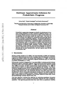
it into a Binary Decision Diagram (BDD), from which we can compute the probability (perform weighted model counting) of the query with a dynamic programming algorithm that is linear in the size of the BDD. A BDD for a function of Boolean variables is a rooted graph that has one level for each Boolean variable. A node n in a BDD has two children: one corresponding to the 1 value of the variable associated with the level of n, indicated with child1 (n), and one corresponding to the 0 value of the variable, indicated with child0 (n). When drawing BDDs, the 0-branch - the one going to child0 (n) - is distinguished from the 1-branch by drawing it with a dashed line. The leaves store either 0 or 1. Figure 1 shows a BDD for the function f (X) = (X1 ∧ X3 ) ∨ (X2 ∧ X3 ), where the variables X = {X1 , X2 , X3 } are independent Boolean random variables whose probability of being true is pi for the variable Xi .
n1
X1
n2
X2 X3
n3 1
0
Fig. 1. BDD representing the function f (X) = (X1 ∧ X3 ) ∨ (X2 ∧ X3 ).
A BDD performs a Shannon expansion of the Boolean formula f (X), so that, if X is the variable associated with the root level of a BDD, the formula f (X) can be represented as f (X) = X ∧ f X (X) ∨ X ∧ f X (X) where f X (X) (f X (X)) is the formula obtained by f (X) by setting X to 1 (0). Now the two disjuncts are pairwise exclusive and the probability of f (X) can be computed as P (f (X)) = P (X)P (f X (X))+(1−P (X))P (f X (X)). Algorithm 2 shows function Prob that implements the dynamic programming algorithm for computing the probability of a formula encoded as a BDD. The function should also store the
Algorithm 2 Computation of the probability of a formula encoded as a BDD. 1: function Prob(node) 2: Input: a BDD node 3: Output: the probability of the Boolean function associated with the node 4: if node is a terminal then 5: return value(node) . value(node) is 0 or 1 6: else 7: let X be v(node) . v(node) is the variable associated with node 8: P1 ←Prob(child1 (node)) 9: P0 ←Prob(child0 (node)) 10: return P (X) · P1 + (1 − P (X)) · P0 11: end if 12: end function
10
value of already visited nodes in a table so that, if a node is visited again, its probability can be retrieved from the table. For the sake of simplicity the algorithm does not show this optimization but it is fundamental to achieve linear cost in the number of nodes, as without it the cost of function Prob would be proportional to 2n where n is the number of Boolean variables. The main BUNDLE function, shown in Algorithm 3, first builds a data structure P M ap that associates each DL axiom Ei with its probability pi . In the OWL files the probabilistic information is specified using the annotation system allowed by the OWL language. Then BUNDLE uses Pellet’s ExpHST(C, K) function that computes all the MinAs for the unsatisfiability of a concept C using the Hitting Set Tree algorithm. BUNDLE exploits the version of this function in which we can specify the maximum number of explanations to be found.
Algorithm 3 Function Bundle: computation of the probability of unsatisfiability of C given K. 1: function Bundle(K, C, maxEx, maxT ime) 2: Input: K (the knowledge base) 3: Input: C (the concept to be tested for unsatisfiability) 4: Input: maxEx (the maximum number of explanations to be found) 5: Input: maxT ime (time limit for the search for explanations) 6: Output: the probability of the unsatisfiability of C w.r.t. K 7: Build Map P M ap from DL axioms to sets of couples (axiom, probability) 8: M inAs ←ExpHST(C, K, maxEx) . Call to Pellet 9: Initialize V arAx to empty . V arAx is an array of couples (Axiom, P rob) 10: BDD ←BDDZero 11: for all M inA ∈ M inAs do 12: BDDE ←BDDOne 13: for all Ax ∈ M inA do 14: p ← P M ap(Ax) 15: Scan V arAx looking for Ax 16: if !found then 17: Add to V arAx a new cell containing (Ax, p) 18: end if 19: Let i be the position of (Ax, p) in V arAx 20: BDDA ← BDDGetIthVar(i) 21: BDDE ←BDDAnd(BDDE,BDDA) 22: end for 23: BDD ←BDDOr(BDD,BDDE) 24: end for 25: return Prob(BDD) . V arAx is used to compute P (X) in Prob 26: end function
Two data structures are initialized: V arAx is an array that maintains the association between Boolean random variables (whose index is the array index) and couples (axiom, probability), and BDD stores a BDD. BDD is initialized to the zero Boolean function. Then BUNDLE performs two nested loops that build a BDD representing the pinpointing formula in DNF. To manipulate BDDs we used JavaBDD3 that is an interface to a number of underlying BDD manipulation packages. As the underlying package we used CUDD. 3
http://javabdd.sourceforge.net/
11
In the outer loop, BUNDLE combines BDDs for different explanations. In the inner loop, BUNDLE generates the BDD for a single explanation. In the outer loop, BDDE is initialized to the “one” Boolean function. In the inner loop, the axioms of each MinA are considered one by one. The value p associated with the axiom is extracted from P M ap. The axiom is searched for in V arAx to see if it was already assigned a random variable. If not, a cell is added to V arAx to store the couple. At this point we know the couple position i in V arAx and so the index of its Boolean variable Xi . We obtain a BDD representing Xi = 1 with BDDGetIthVar and we conjoin it with BDDE. After the two cycles, function Prob of Algorithm 2 is called over BDD and its result is returned to the user.
6
TRILL
TRILL implements a tableau algorithm that computes the pinpointing formula representing the set of MinAs. After generating the pinpointing formula, TRILL converts it into a BDD and computes the probability of the query. TRILL can answer concept and role membership queries, subsumption queries, and can find explanations both for the unsatifiability of a concept contained in the KB and for the inconsistency of the entire KB. TRILL was implemented in Prolog, so the management of the non-determinism of the rules is delegated to this language. We use the Thea2 library [45] for converting OWL DL KBS into Prolog. Thea2 performs a direct translation of the OWL axioms into Prolog facts. For example, a simple subclass axiom between two named classes Cat v P et is written using the subClassOf/2 predicate as subClassOf(‘Cat’,‘Pet’). For more complex axioms, Thea2 exploits the list construct of Prolog, so the axiom N atureLover ≡ P etOwnertGardenOwner becomes equivalentClasses( [‘NatureLover’, unionOf([‘PetOwner’, ‘GardenOwner’])]). When a probabilistic KB is given as input, for each probabilistic axiom of the form P rob :: Axiom a fact p(Axiom,Prob) is asserted in the Prolog KB. In order to represent the tableau, TRILL uses a couple T ableau = (A, T ), where A is a list containing information about nominal individuals and class assertions with the corresponding value of the pinpointing formula, while T is a triple (G, RBN , RBR) in which G is a directed graph that contains the structure of the tableau, RBN is a red-black tree (a key-value dictionary) in which a key is a couple of individuals and its value is the set of the labels of the edge between the two individuals, and RBR is a red-black tree in which a key is a role and its value is the set of couples of individuals that are linked by the role. This representation allows to quickly find the information needed during the execution of the tableau algorithm. For managing the blocking system we use a predicate for each blocking state: nominal/2, blockable/2, blocked/2, indirectly blocked/2 and safe/3. Each predicate takes as arguments the individual Ind and the tableau (A, T ); safe/3 takes as input also the role R. For each individual Ind in the ABox we add the atom nominal(Ind) to A, then 12
every time we have to check the blocking status of an individual we call the corresponding predicate that returns the status by checking the tableau. Deterministic and non-deterministic tableau expansion rules are treated differently. Non-deterministic rules are implemented by a predicate rule name(T ab, T abList) that, given the current tableau T ab, returns the list of tableaux T abList created by the application of the rule on T ab, while deterministic rules are implemented by a predicate rule name(T ab, T ab1) that, given the current tableau T ab, returns the tableau T ab1 obtained by the application of the rule on T ab. Expansion rules are applied in order by apply all rules/2, first the nondeterministic ones and then the deterministic ones. The predicate apply nondet rules(RuleList,Tab,Tab1) takes as input the list of non-deterministic rules and the current tableau and returns a tableau obtained by the application of one of the rules. apply nondet rules/3 is called as apply nondet rules([or rule],Tab,Tab1) and is shown in Figure 2. If a non-
apply_all_rules(Tab,Tab2):apply_nondet_rules([or_rule],Tab,Tab1), (Tab=Tab1 -> Tab2=Tab1 ; apply_all_rules(Tab1,Tab2)).
apply_nondet_rules([],Tab,Tab1):apply_det_rules([and_rule,unfold_rule,add_exists_rule, forall_rule,exists_rule],Tab,Tab1). apply_nondet_rules([H|T],Tab,Tab1):C=..[H,Tab,L], call(C),! member(Tab1,L), Tab \= Tab1. apply_nondet_rules([_|T],Tab,Tab1):apply_nondet_rules(T,Tab,Tab1).
Fig. 2. Definition of the non-deterministic expansion rules by means of the predicates apply all rules/2 and apply nondet rules/3.
deterministic rule is applicable, the list of tableaux obtained by its application is returned by the predicate corresponding to the applied rule, a cut is performed to avoid backtracking to other rule choices and a tableau from the list is non-deterministically chosen with the member/2 predicate. If no non-deterministic rule is applicable, deterministic rules are tried sequentially with the predicate apply det rules/3, shown in Figure 3, that is called as apply det rules(RuleList,Tab,Tab1). It takes as input the list of 13
deterministic rules and the current tableau and returns a tableau obtained with the application of one of the rules. After the application of a deterministic rule, a cut avoids backtracking to other possible choices for the deterministic rules. If no rule is applicable, the input tableau is returned and rule application stops, otherwise a new round of rule application is performed. apply_det_rules([],Tab,Tab). apply_det_rules([H|T],Tab,Tab1):C=..[H,Tab,Tab1], call(C),!. apply_det_rules([_|T],Tab,Tab1):apply_det_rules(T,Tab,Tab1).
Fig. 3. Definition of the deterministic expansion rules by means of the predicate apply det rules/3.
Once the pinpointing formula is built, TRILL builds the correponding BDD by using the build bdd/2 predicate, shown in Figure 4, that takes as input a pinpointing formula and returns the correspondig BDD. It scans the pinpointing formula and, for each variable, it searches for the probabilistic axiom corresponding to the variable with the query p(Axiom,Prob). If the query succeeds, it creates the corresponding BDD and combines it with the BDD representing the pinpointing formula. Finally, it computes the probability of the query from the BDD so built using the predicate compute prob/2. The predicates one/1 and zero/1 return BDDs representing the Boolean constants 1 and 0; and/3 and or/3 execute Boolean operations between BDDs. get var n/4 returns the random variable associated with axiom X and list of probabilities [Prob,ProbN], where ProbN = 1 − Prob. equality/3 returns the BDD B associated with the expression VX=val where VX is a random variable and val is 0 or 1. The predicate p/2 is used for specifying the association between axioms and probability, i.e. p(subClassOf(’A’,’B’),0.9) asserts the axiom A v B is associated with a probability of 0.9. The predicates compute prob/2, one/1, zero/1, and/3, or/3, get var n/4 and equality/3 are imported from a Prolog library of the cplint suite [33].
7
Related Work
While there are many works that propose approaches for combining probability and DLs, there are relatively fewer inference algorithms. One of these is PRONTO [21] that, similarly to BUNDLE, is based on Pellet. PRONTO performs inference on P-SHIQ(D) [25] KBs instead of DISPONTE. In these KBs 14
build_bdd(and(A),B):-!, one(B0), bdd_and(A,B0,B). build_bdd(or(A),B):-!, zero(B0), bdd_or(A,B0,B). build_bdd(A,B):p(A,Prob),!, ProbN is 1-Prob, get_var_n([X],[],[Prob,ProbN],VX), equality(VX,0,B). build_bdd(A,B):one(B). bdd_and([],B,B). bdd_and([H|T],B0,B):build_bdd(H,B1), and(B0,B1,B2), bdd_and(T,B2,B). bdd_or([],B,B). bdd_or([H|T],B0,B):build_bdd(H,B1), or(B0,B1,B2), bdd_or(T,B2,B).
Fig. 4. Code of the predicates build bdd rules/2.
15
the probabilistic part contains conditional contraints of the form (D|C)[l, u] that informally mean “generally, if an object belongs to C, then it belongs to D with a probability in the interval [l, u]”. P-SHIQ(D) uses probabilistic lexicographic entailment from probabilistic default reasoning and allows both terminological and assertional probabilistic knowledge about instances of concepts and roles. PSHIQ(D) is based on Nilsson’s probabilistic logic [27] that defines probabilistic interpretations instead of a single probability distribution over theories. Differently from BUNDLE and PRONTO, reasoners written in Prolog can exploit Prolog’s backtracking facilities for performing the search. This has been observed in various work. Beckert and Posegga [6] proposed a tableau reasoner in Prolog for First Order Logic (FOL) based on free-variable semantic tableaux. However, the reasoner is not tailored to DLs. Hustadt, Motik and Sattler [17] presented the KAON2 algorithm that exploits basic superposition, a refutational theorem proving method for FOL with equality, and a new inference rule, called decomposition, to reduce a SHIQ KB into a disjunctive datalog program, while DLog [24] is an ABox reasoning algorithm for the SHIQ language that allows to store the content of the ABox externally in a database and to answer instance check and instance retrieval queries by transforming the KB into a Prolog program. Meissner [26] presented the implementation of a Prolog reasoner for the DL ALCN . This work was the basis of the work of Herchenr¨oder [15], that considered ALC and improved the work of Meissner by implementing heuristic search techniques to reduce the running time. Faizi [10] added to [15] the possibility of returning information about the steps executed during the inference process for queries but still handled only ALC. A different approach is the one of Ricca et al. [32] that presented OntoDLV, a system for reasoning on a logic-based ontology representation language called OntoDLP. This is an extension of (disjunctive) ASP and can interoperate with OWL. OntoDLV rewrites the OWL KB into the OntoDLP language, can retrieve information directly from external OWL Ontologies and answers queries by using ASP. TRILL differs from the previous works for the target description logics (ALC) and for the fact that those reasoners do not return explanations for the given queries. Moreover, TRILL differs in particular from DLog for the possibility of answering general queries instead of instance check and instance retrieval only.
8
Experiments
In this section, we evaluate the performance of TRILL and BUNDLE. We first compare BUNDLE with the publicly available version of PRONTO on four probabilistic ontologies. The experiments have been performed on Linux machines with a 3.10 GHz Intel Xeon E5-2687W with 2GB memory allotted to Java. The first ontology is BRCA4 that models breast cancer risk assessment. It contains a certain part and a probabilistic part. The tests were defined following 4
http://www2.cs.man.ac.uk/~klinovp/pronto/brc/cancer_cc.owl
16
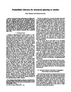
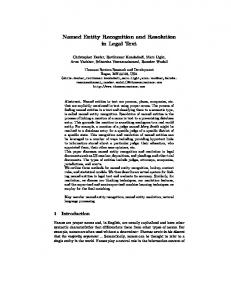
[22]: we randomly sampled axioms from the probabilistic part of this ontology which are then added to the certain part. So each sample was a probabilistic KB with the full certain part of the BRCA ontology and a subset of the probabilistic constraints. We varied the number of these constraints from 9 to 15, and, for each number, we generated 100 different consistent ontologies. In order to generate a query, an individual a is added to the ontology. a is randomly assigned to each class that appears in the sampled conditional constraints with probability 0.6. If the class is composite, as for example PostmenopausalWomanTakingTestosterone, a is assigned to the component classes rather than to the composite one. In the example above, a will be added to PostmenopausalWoman and WomanTakingTestosterone. The ontologies are then translated into DISPONTE by replacing the constraint (D|C)[l, u] with the axiom u :: C v D. For each ontology we perform the query a : C where the class C is randomly selected among those that represent women under increased and lifetime risk such as WomanUnderLifetimeBRCRisk and WomanUnderStronglyIncreasedBRCRisk. We then applied both BUNDLE and PRONTO to each generated test and we measured the execution time and the memory used. Figure 5(a) shows the execution time averaged over the 100 KBs as a function of the number of probabilistic axioms and, similarly, Figure 5(b) shows the average amount of memory used. As one can see, execution times are similar for small KBs, but the difference between the two reasoners rapidly increases for larger knowledge bases. The memory usage for BUNDLE is always less than 53% with respect of PRONTO.
(a) Average execution times (s).
(b) Average memory used (Kb).
Fig. 5. Comparison between BUNDLE and PRONTO on the BRCA KB.
The other three ontologies are an extract from the Cell5 ontology that represents cell types of the prokaryotic, fungal, and eukaryotic organisms, an extract 5
http://cellontology.org/
17
from the NCI Thesaurus6 that describes human anatomy and an extract from the Teleost anatomy7 ontology (Teleost for short) that is a multi-species anatomy ontology for teleost fishes. For each of these KBs we considered the versions of increasing size used in [23]: the authors added 250, 500, 750 and 1000 new probabilistic conditional constraints to the extract of the publicly available nonprobabilistic version of each ontology. We converted these KBs into DISPONTE in the same way presented for the BRCA ontology and we created a set of 100 different random subclass queries for each KB, such as CL 0000802 v CL 0000800 for the Cell KB, N CI C32042 v N CI C32890 for the NCI Thesaurus and T AO 0001102 v T AO 0000139 for the Teleost KB. For generating the queries we built the hierarchy of each KB and we randomly selected two classes connected in the hierarchy for each query, so that it had at least one explanation. In Table 1 we report, for each version of the datasets, the average execution time for BUNDLE to perform inference. In addition, for each KB we report its number of non-probabilistic TBox axioms. With these datasets, PRONTO always terminated with out-of-memory error.
Probabilistic TBox Size Dataset TBox axioms 0 250 500 750 1000 Cell 1263 time(s) 0.76 2.84 3.88 3.94 4.53 Teleost 3406 time(s) 2.11 8.87 31.80 33.82 36.33 NCI 5423 time(s) 3.02 11.37 11.37 16.37 24.90 Table 1. Average execution time for the queries to the Cell, Teleost and NCI KBs. The first column reports the size of the non-probabilistic TBox of each KB.
As can be seen, BUNDLE needs lower amount of memory and is faster than the publicly available version of PRONTO. BUNDLE can answer most queries in a few seconds and manage larger KBs with respect to PRONTO. Finally, we tested TRILL performance when computing probability of queries by comparing it to BUNDLE. The experiments have been performed on a Linux machine with a 2.33 GHz Intel Dual Core E6550 with 2GB memory allotted to Java. We consider four different knowledge bases of various complexity: BRCA already used for the comparison with PRONTO, an extract of the DBPedia8 ontology obtained from Wikipedia, Biopax level 39 that models metabolic pathways and Vicodi10 that contains information about European history. For the tests, we used the DBPedia and the Biopax KBs without ABox while for BRCA and Vicodi we used a small ABox contaning 1 individual for the first one and 19 individuals for the second one. We added 50 probabilistic axioms to each KB. For 6 7 8 9 10
http://ncit.nci.nih.gov/ http://phenoscape.org/wiki/Teleost_Anatomy_Ontology http://dbpedia.org/ http://www.biopax.org/ http://www.vicodi.org/
18
BRCA we used the probabilistic axioms already created for the previous test, while for the other KBs we created the probabilistic axioms by randomly selecting certain axioms from them and associating a random probability. For each dataset we randomly created 100 different queries. In particular, for the DBPedia and Biopax we created 100 subclass-of queries while for the other KBs we created 80 subclass-of and 20 instance-of queries. Some examples of queries are V illage v P opulatedP lace for DBPedia, T ransportW ithBiochemicalReaction v Entity for Biopax and Creator(Anthony-van-Dyck-is-Painter-in-Flanders) for Vicodi KB. The queries generated for the BRCA KB are similar with those used in the test of BUNDLE. For generating the subclass-of queries, we randomly selected two classes that are connected in the class hierarchy, while for the instance-of queries we randomly selected an individual a and a class to which a belongs by following the class hierarchy, starting from the class to which a explicitly belongs, so that each query had at least one explanation. Table 2 shows, for each ontology, the number of non-probabilistic axioms and the average time in seconds that TRILL and BUNDLE took for answering the queries. These preliminary tests show that TRILL is sometimes able to outperform BUNDLE, thanks to the fact that the translation of the set of explanations into a DNF formula is not required. However, on DBPedia, its longer running time may be due to the lack of all the optimizations that BUNDLE inherits from Pellet. This represents evidence that a Prolog implementation of a Semantic Web tableau reasoner is feasible and that may lead to a practical system. TRILL BUNDLE Dataset TBox axioms time(s) time(s) BRCA 322 5.55 6.96 DBPedia 535 16.70 3.79 Biopax level 3 826 0.11 1.85 Vicodi 220 0.19 1.12 Table 2. Results of the experiments on BRCA, DBPedia, Biopax and Vicodi KBs in terms of average times for computing the probability of queries. The first column reports the size of the non-probabilistic TBox of each KB.
9
Conclusions
In this paper we presented the DISPONTE semantics for probabilistic DLs that is inspired by the distribution semantics of probabilistic logic programming. We also presented the systems BUNDLE and TRILL for reasoning on DISPONTE KBs and their implementations. Both systems are tested on real world datasets. The experiments show that BUNDLE uses less memory and is faster than the publicly available version of the probabilistic reasoner PRONTO and is able to manage larger KBs. Moreover, the results for TRILL show that Prolog is a viable 19
language for implementing DL reasoning algorithms and that its performance is comparable with that of a state-of-the-art reasoner. Both TRILL and BUNDLE are able to deal with ontologies of significant complexity.
References 1. Baader, F., Calvanese, D., McGuinness, D.L., Nardi, D., Patel-Schneider, P.F. (eds.): The Description Logic Handbook: Theory, Implementation, and Applications. Cambridge University Press (2003) 2. Baader, F., Horrocks, I., Sattler, U.: Description logics. In: Handbook of knowledge representation, chap. 3, pp. 135–179. Elsevier (2008) 3. Baader, F., Pe˜ naloza, R.: Automata-based axiom pinpointing. J. Autom. Reasoning 45(2), 91–129 (2010) 4. Baader, F., Pe˜ naloza, R.: Axiom pinpointing in general tableaux. J. Log. Comput. 20(1), 5–34 (2010) 5. Bacchus, F.: Representing and reasoning with probabilistic knowledge - a logical approach to probabilities. MIT Press (1990) 6. Beckert, B., Posegga, J.: leantap: Lean tableau-based deduction. J. Autom. Reasoning 15(3), 339–358 (1995) 7. Bellodi, E., Lamma, E., Riguzzi, F., Albani, S.: A distribution semantics for probabilistic ontologies. In: International Workshop on Uncertainty Reasoning for the Semantic Web. No. 778 in CEUR Workshop Proceedings, Sun SITE Central Europe (2011) 8. Darwiche, A., Marquis, P.: A knowledge compilation map. J. Artif. Intell. Res. 17, 229–264 (2002) 9. De Raedt, L., Kimmig, A., Toivonen, H.: ProbLog: A probabilistic Prolog and its application in link discovery. In: International Joint Conference on Artificial Intelligence. pp. 2462–2467 (2007) 10. Faizi, I.: A Description Logic Prover in Prolog, Bachelor’s thesis, Informatics Mathematical Modelling, Technical University of Denmark (2011) 11. Gomes, C.P., Sabharwal, A., Selman, B.: Model counting. In: Biere, A. (ed.) Handbook of Satisfiability. IOS Press (2008) 12. Haarslev, V., Hidde, K., M¨ oller, R., Wessel, M.: The racerpro knowledge representation and reasoning system. Semantic Web 3(3), 267–277 (2012) 13. Halaschek-Wiener, C., Kalyanpur, A., Parsia, B.: Extending tableau tracing for ABox updates. Tech. rep., University of Maryland (2006) 14. Halpern, J.Y.: An analysis of first-order logics of probability. Artif. Intell. 46(3), 311–350 (1990) 15. Herchenr¨ oder, T.: Lightweight Semantic Web Oriented Reasoning in Prolog: Tableaux Inference for Description Logics. Master’s thesis, School of Informatics, University of Edinburgh (2006) 16. Hitzler, P., Kr¨ otzsch, M., Rudolph, S.: Foundations of Semantic Web Technologies. CRCPress (2009) 17. Hustadt, U., Motik, B., Sattler, U.: Deciding expressive description logics in the framework of resolution. Inf. Comput. 206(5), 579–601 (2008) 18. Kalyanpur, A.: Debugging and Repair of OWL Ontologies. Ph.D. thesis, The Graduate School of the University of Maryland (2006) 19. Kalyanpur, A., Parsia, B., Horridge, M., Sirin, E.: Finding all justifications of OWL DL entailments. In: International Semantic Web Conference. LNCS, vol. 4825, pp. 267–280. Springer (2007)
20
20. Kalyanpur, A., Parsia, B., Sirin, E., Hendler, J.A.: Debugging unsatisfiable classes in OWL ontologies. J. Web Sem. 3(4), 268–293 (2005) 21. Klinov, P.: Pronto: A non-monotonic probabilistic description logic reasoner. In: European Semantic Web Conference. LNCS, vol. 5021, pp. 822–826. Springer (2008) 22. Klinov, P., Parsia, B.: Optimization and evaluation of reasoning in probabilistic description logic: Towards a systematic approach. In: International Semantic Web Conference. LNCS, vol. 5318, pp. 213–228. Springer (2008) 23. Klinov, P., Parsia, B.: A hybrid method for probabilistic satisfiability. In: Bjørner, N., Sofronie-Stokkermans, V. (eds.) International Conference on Automated Deduction. LNCS, vol. 6803, pp. 354–368. Springer (2011) 24. Luk´ acsy, G., Szeredi, P.: Efficient description logic reasoning in prolog: The dlog system. TPLP 9(3), 343–414 (2009) 25. Lukasiewicz, T.: Expressive probabilistic description logics. Artif. Int. 172(6-7), 852–883 (2008) 26. Meissner, A.: An automated deduction system for description logic with alcn language. Studia z Automatyki i Informatyki 28-29, 91–110 (2004) 27. Nilsson, N.J.: Probabilistic logic. Artif. Intell. 28(1), 71–87 (1986) 28. Patel-Schneider, P, F., Horrocks, I., Bechhofer, S.: Tutorial on OWL (2003) 29. Poole, D.: The Independent Choice Logic for modelling multiple agents under uncertainty. Artif. Intell. 94(1-2), 7–56 (1997) 30. Poole, D.: Probabilistic horn abduction and Bayesian networks. Artif. Intell. 64(1) (1993) 31. Reiter, R.: A theory of diagnosis from first principles. Artif. Intell. 32(1), 57–95 (1987) 32. Ricca, F., Gallucci, L., Schindlauer, R., Dell’Armi, T., Grasso, G., Leone, N.: Ontodlv: An asp-based system for enterprise ontologies. J. Log. Comput. 19(4), 643– 670 (2009) 33. Riguzzi, F.: Extended semantics and inference for the Independent Choice Logic. Log. J. IGPL 17(6), 589–629 (2009) 34. Riguzzi, F., Bellodi, E., Lamma, E.: Probabilistic Datalog+/- under the distribution semantics. In: Kazakov, Y., Lembo, D., Wolter, F. (eds.) International Workshop on Description Logics (2012) 35. Riguzzi, F., Bellodi, E., Lamma, E., Zese, R.: Computing instantiated explanations in owl dl. In: Baldoni, M., Baroglio, C., Boella, G., Micalizio, R. (eds.) AI*IA. Lecture Notes in Computer Science, vol. 8249, pp. 397–408. Springer (2013) 36. Riguzzi, F., Bellodi, E., Lamma, E., Zese, R.: Probabilistic description logics under the distribution semantics. Semantic Web Journal (2014), to appear 37. Riguzzi, F., Lamma, E., Bellodi, E., Zese, R.: Epistemic and statistical probabilistic ontologies. In: Uncertainty Reasoning for the Semantic Web. CEUR Workshop Proceedings, vol. 900, pp. 3–14. Sun SITE Central Europe (2012) 38. Sang, T., Beame, P., Kautz, H.A.: Performing bayesian inference by weighted model counting. In: Proceedings of AAAI. pp. 475–482. AAAI Press / The MIT Press, Palo Alto, CA, Pittsburgh, PA (9-13 July 2005) 39. Sato, T.: A statistical learning method for logic programs with distribution semantics. In: International Conference on Logic Programming. pp. 715–729. MIT Press (1995) 40. Sato, T., Kameya, Y.: Parameter learning of logic programs for symbolic-statistical modeling. J. Artif. Intell. Res. 15, 391–454 (2001)
21
41. Schlobach, S., Cornet, R.: Non-standard reasoning services for the debugging of description logic terminologies. In: International Joint Conference on Artificial Intelligence. pp. 355–362. Morgan Kaufmann (2003) 42. Schmidt-Schauß, M., Smolka, G.: Attributive concept descriptions with complements. Artificial Intelligence 48(1), 1–26 (1991) 43. Shearer, R., Motik, B., Horrocks, I.: Hermit: A highly-efficient owl reasoner. In: OWLED (2008) 44. Sirin, E., Parsia, B., Cuenca-Grau, B., Kalyanpur, A., Katz, Y.: Pellet: A practical OWL-DL reasoner. J. Web Sem. 5(2), 51–53 (2007) 45. Vassiliadis, V., Wielemaker, J., Mungall, C.: Processing owl2 ontologies using thea: An application of logic programming. In: International Workshop on OWL: Experiences and Directions. CEUR Workshop Proceedings, vol. 529. CEUR-WS.org (2009) 46. Vennekens, J., Denecker, M., Bruynooghe, M.: CP-logic: A language of causal probabilistic events and its relation to logic programming. Theory Pract. Log. Program. 9(3), 245–308 (2009) 47. Vennekens, J., Verbaeten, S., Bruynooghe, M.: Logic programs with annotated disjunctions. In: International Conference on Logic Programming. LNCS, vol. 3131, pp. 195–209. Springer (2004)
22