Angle-based Space Partitioning for Efficient Parallel Skyline ...

Angle-based Space Partitioning for Efficient Parallel Skyline Computation ∗

Akrivi Vlachou , Christos Doulkeridis, Yannis Kotidis

Department of Informatics, Athens University of Economics and Business, Greece

ABSTRACT Recently, skyline queries have attracted much attention in the database research community. Space partitioning techniques, such as recursive division of the data space, have been used for skyline query processing in centralized, parallel and distributed settings. Unfortunately, such grid-based partitioning is not suitable in the case of a parallel skyline query, where all partitions are examined at the same time, since many data partitions do not contribute to the overall skyline set, resulting in a lot of redundant processing. In this paper we propose a novel angle-based space partitioning scheme using the hyperspherical coordinates of the data points. We demonstrate both formally as well as through an exhaustive set of experiments that this new scheme is very suitable for skyline query processing in a parallel sharenothing architecture. The intuition of our partitioning technique is that the skyline points are equally spread to all partitions. We also show that partitioning the data according to the hyperspherical coordinates manages to increase the average pruning power of points within a partition. Our novel partitioning scheme alleviates most of the problems of traditional grid partitioning techniques, thus managing to reduce the response time and share the computational workload more fairly. As demonstrated by our experimental study, our technique outperforms grid partitioning in all cases, thus becoming an efficient and scalable solution for skyline query processing in parallel environments.

Categories and Subject Descriptors H.2.4 [Database Management]: Systems—Query processing, Parallel databases

General Terms Algorithms, Experimentation, Performance ∗This research project is co-financed by E.U.-European Social Fund (75%) and the Greek Ministry of DevelopmentGSRT (25%).

Permission to make digital or hard copies of all or part of this work for personal or classroom use is granted without fee provided that copies are not made or distributed for profit or commercial advantage and that copies bear this notice and the full citation on the first page. To copy otherwise, to republish, to post on servers or to redistribute to lists, requires prior specific permission and/or a fee. SIGMOD’08, June 9–12, 2008, Vancouver, BC, Canada. Copyright 2008 ACM 978-1-60558-102-6/08/06 ...$5.00.

price (y)

{avlachou,cdoulk,kotidis}@aueb.gr

10

g c

j

d

i

f 5

e a k

h

b

0 0

5

10

distance (x)

Figure 1: Skyline Example

Keywords Skyline operator, parallel computation, space partitioning

1. INTRODUCTION Skyline queries [2] have attracted much attention recently, since they help users to make intelligent decisions over complex data, where many conflicting criteria are considered. Consider for example a database containing information about hotels. Each tuple of the database is represented as a point in a data space consisting of numerous dimensions. In our example, the y-dimension represents the price of a room, whereas the x-dimension captures the distance of the hotel to a point of interest such as the beach (Figure 1). According to the dominance definition, a hotel dominates another hotel because it is cheaper and closer to the beach. Thus, the skyline points are the best possible tradeoffs between price and distance from the beach. Space partitioning techniques, such as recursive division of the data space, have been used for skyline query processing in centralized [2], parallel [21] and distributed [19] settings. This grid-based partitioning technique seems to become a widely accepted data partitioning method for skyline computation in distributed environments. The goals of these partitioning techniques is to divide the data space or the data points into partitions, in order to make it fit into main memory [2] or to divide the workload among different servers [19, 21]. Thereafter, the query is executed on each partition and merged into a global result set. The main advantage of the grid partitioning technique is that some data space partitions may not be examined, when the query is executed in a partially serialized manner. However, in the case

price (y)

price (y)

10

g c

j

d

10

g c

j

d

i

f 5

i

f 5

e

e

a

a k

h

k b

0

h

b

0 0

5

10

0

5

distance (x)

(a) Angle partitioning

10

distance (x)

(b) Grid partitioning

Figure 2: Partitioning example.

of parallel processing of the skyline query, where all partitions are examined simultaneously, the performance of grid partitioning degrades. This is mainly because many partitions do not contribute to the global result set (or contribute marginally), resulting in a lot of redundant processing. With the explosive increase of available data, parallelizing costly query operators, such as the skyline operator, which is CPU-intensive [2, 3], is important in order to retrieve the results in reasonable response time. Centralized skyline algorithms have the disadvantage that response time increases rapidly (up to quadratic) with the cardinality of the dataset. Therefore, a centralized algorithm becomes inappropriate when massive amounts of data have to be processed. Parallel query processing attempts to alleviate some of the deficiencies of such problematic situations and has been explored by the database research community for other operators such as joins, nearest neighbor queries, etc. Although the skyline operator has been thoroughly investigated in centralized settings [2, 4, 10, 14, 17], only recently parallel [5, 6, 21] and distributed [1, 7, 18, 19] skyline query processing has attracted attention. In this paper, we address the problem of how to compute efficiently skyline queries over a set of N servers in parallel. We focus on the important issue of how to partition the dataset to the N servers, in order to increase the efficiency of skyline query processing. In our setting, queries arrive at a central node, which is also called the coordinator server, that distributes the processing requests to all participating servers and collects their results. The query is executed simultaneously on all servers. Our objectives are to minimize the response time and share the processing load evenly. In this spirit, we propose a novel angle-based partitioning scheme that alleviates many of the shortcomings of gridbased partitioning. We first transform the coordinates of each point of the dataset to hyperspherical coordinates and then we apply grid partitioning on the respective angular coordinates. This approach results in space partitions that are more homogeneous with respect to skyline processing, than in the case of grid partitioning where some partitions are more important and others are non-contributing. Consider the example depicted in Figure 2. The dataset is partitioned over four servers, in Figure 2(a) using the angle-based partitioning technique, while in Figure 2(b) using grid partitioning. The black points are the global skyline points returned to the user. For the angle-partitioning, each partition retrieves only few local skyline points and the majority of them are also skyline points of the entire dataset, while for the grid partitioning some of the partitions (such as the

upper right) do not contribute to the skyline result set at all. In this example, the angle-based partitioning scheme gathers 6 local skyline points and 5 of them are the global skyline points, while the grid approach results 11 local skyline points. Thus, the total number of local skyline points, that need to be processed by the coordinator node in order to compute the 5 global skyline points, is much higher in the case of the grid partitioning. Therefore, the post-processing cost is significantly lower for the angle-based partitioning. Another important feature of our partitioning scheme is that the average pruning power of a local data point is much higher, compared to the case of grid partitioning. While we defer a detailed analysis to Section 5, in Figure 2 we can see that points a and k dominate all other points in their respective partition. This property results in per-partition processing times that are much lower compared to the case of grid partitioning. This intuition is also demonstrated in our experimental evaluation. To summarize, the contributions of this paper are the following: • We present a novel partitioning method that uses the hyperspherical coordinates for parallelizing skyline query processing over a set of servers, in a deliberate way, such that response time decreases significantly and the processing load is evenly distributed among servers. • We show both formally as well as experimentally that our method is particularly suitable for skyline computation, as it distributes the global skyline points evenly to all partitions while preserving their pruning power. • We present two algorithms that utilize the novel anglebased partitioning scheme for distributing evenly the dataset among the servers. The first is intented for uniform datasets and partitions the space in equal volumes, whereas the second works for arbitrary data distributions. • We provide an extensive comparative experimental evaluation demonstrating the advantages of our partitioning scheme over the widely employed grid partitioning technique for parallel skyline computation. We are up to 10 times better than grid in terms of response time and constantly outperform both grid and random partitioning. The outline of this paper is the following: in Section 2, the related work is presented. Section 3 presents the preliminaries, while in Section 4, we state the problem tackled in this work. In Section 5, we introduce our angle-based partitioning scheme for parallel skyline query processing. Then, in Section 6, we present two algorithms that utilize the angle partitioning approach, namely for uniform and for arbitrary data distributions. In Section 7 we present an extensive experimental evaluation of the proposed techniques, and finally in Section 8 we conclude the paper and sketch future research directions.

2. RELATED WORK Skyline computation has recently attracted considerable attention in the database research community. B¨ orzs¨ onyi et al. [2] first investigate the skyline computation problem in the context of databases. They proposed the BNL [2] algorithm that compares each point of the database with

every other point, and reports it as a result only if it is not dominated by any other point. D&C [2] divides the data space into several regions, calculates the skyline in each region, and produces the final skyline from the points in the regional skylines. SFS [4], which is based on the same principle as BNL, improves performance by first sorting the data according to a monotone function. Thereafter, index-based techniques are proposed in several works. Tan et al. [17] propose the first progressive techniques, namely Bitmap and Index method. In [10], an algorithm based on nearest neighbor search on the indexed dataset is presented. Then, Papadias et al. [14] propose a branch and bound algorithm to progressively output skyline points from a dataset indexed by an R-Tree, with guaranteed minimum I/O cost. There has been a growing interest in distributed [1, 7, 12, 18, 19] and parallel [5, 6, 21] skyline computation lately. In [1, 12], skyline processing is studied over distributed web sources. In both cases, the authors assume vertical partitioning of the dataset across a set of participating web accessible sources. This is entirely different from out setup, where the aim is to distribute the dataset horizontally to a set of N servers. Skylines have been studied in other distributed contexts as well. Huang et al. [8] assume a setting with mobile devices communicating via an ad-hoc network (MANETs), and study skyline queries that involve spatial constraints. The authors present techniques that aim to reduce both the communication cost and the execution time on each single device. In [18], the authors study the problem of subspace skyline processing in a super-peer network, where peers hold their data in an autonomous manner and collectively process skyline queries on subspaces. Both approaches do not address the issue of space partitioning. In [7], the authors focus on Peer Data Management Systems (PDMS), where each peer provides its own data with its own schema. Their techniques provide probabilistic guarantees for the result’s correctness. There are also several approaches for P2P skyline computation that apply space partitioning techniques. Wang et al. [19] use the z-curve method to map the multidimensional data space to one dimensional values, that can then be assigned to peers connected in a tree overlay like BATON [9]. In this approach, due to the space partitioning scheme, there arises a load balancing problem. In particular, a small number of peers (those that were allocated space near the origin of the axes) eventually have to process almost every query. In order to improve the performance the authors propose extensions such as smaller space allocation to peers responsible for these regions or data replication techniques. However, this partitioning technique is not efficient for parallel skyline computation, since many servers that do not contribute to the skyline result set are queried. Li et al. [11] use a space partitioning method that is based on an underlying semantic overlay (Semantic Small World - SSW). Their approach shares the same drawbacks as [19], as the main difference is only the use of SSW instead of a tree structure. In [21], Wu et al. first address the problem of parallelizing skyline queries over a share-nothing architecture. The proposed algorithm named DSL, relies on space partitioning techniques. The author propose two mechanisms, recursive region partitioning and dynamic region encoding. Their techniques enforce the skyline partial order, so that the sys-

Symbols P d n N Si Di Pi pi SKYPi φi

Description Dataset Data dimensionality Dataset cardinality Number of partitions i-th server i-th data space partition Points of i-th partition i-th coordinate of point p Skyline set of partition Pi i-th angular coordinate

Table 1: Overview of symbols.

tem pipelines participating machines during query execution and minimizes inter-machine communication. In contrast to our approach where all servers process the query at the same time, in [21] each server starts the skyline computation on its data after receiving the results of other servers based on the partial order. Parallel skyline computation is also studied in [5]. The algorithm first partitions the dataset in a random way to the participating machines, in order to ensure that the structure of each partition is similar to the original dataset. Then each machine processes the skyline over its local data using an R-Tree as indexing structure. We explore the random partitioning technique in our experiments and we show that our method partitions the dataset in a way that improves the total response time. A different approach regarding parallel skyline computation is presented in [6]. In contrast to the previous approaches, the authors use a multi-disk architecture with one processor and they use the parallel R-Tree. The main focus of this paper is to access more entries from several disks simultaneously, in order to improve the pruning of non-qualifying points. The authors focus on the efficient distribution of the nodes of the parallel R-Tree, while our approach focuses on the data space partitioning problem for a parallel share-nothing architecture. To summarize, most research papers that apply a space partitioning scheme for distributed or parallel skyline processing rely on a grid-based partitioning. For example, in [21], space is partitioned based on CAN [15], whereas in [19] a tree-structured overlay, is used to partition the data space to peers. While this type of partitioning has some attractive features (small number of peers necessary to process a skyline query), it suffers from poor load balancing, causing few peers to carry all the processing burden, while most peers are practically idle. While in a peer-to-peer network the focus is on minimizing the number of participating peers at query time, in a parallel share-nothing architecture the query is processed simultaneously by all participating servers and we need to minimize the response time by sharing the workload evenly to the servers.

3. PRELIMINARIES Given a data space D defined by a set of d dimensions {d1 , ..., dd } and a dataset P on D with cardinality n, a point p ∈ P can be represented as p = {p1 , ..., pd } where pi is a value on dimension di . Without loss of generality, let us assume that the value pi in any dimension di is greater or equal to zero (pi ≥ 0) and that for all dimensions the minimum values are more preferable.

describe our sub-goals for the parallel skyline algorithm. Skyline Definition: A point p ∈ P is said to dominate another point q ∈ P , denoted as p ≺ q, if (1) on every dimension di ∈ D, pi ≤ qi ; and (2) on at least one dimension dj ∈ D, pj < qj . The skyline is a set of points SKYP ⊆ P which are not dominated by any other point in P . The points in SKYP are called skyline points. Let us further assume a set of N servers Si participating in the parallel computation. The dataset P is horizontally distributed to the N partitions based on a space partitioning technique, suchthat Pi is the set of points stored by server Si where Pi ⊆ P , 1≤i≤N Pi = P and Pi ∩ Pj = ∅ for all i = j. Observation: A point p ∈ P is a skyline point p ∈ SKYP if and only if there exists a partition Pi (1 ≤ i ≤ N ) with p ∈ Pi ⊆ P and p ∈ SKYPi . In other words, the skyline points over a horizontally partitioned dataset are a subset of the union of the skyline points of all partitions. Each server Si computes locally the skyline set SKYPi (mentioned also as local skyline points) based on the locally stored points Pi . In a second phase, the local skylines are merged to the global skyline set, by computing the skyline of the local skyline sets. The above observation guarantees that the parallel skyline algorithm returns the exact skyline set, after merging the local skyline results sets independently from the partitioning algorithm. For a complete reference to the symbols see Table 1.

4.

PROBLEM STATEMENT

Consider a parallel share-nothing architecture. In the typical case, there exists one central server, called coordinator, which is responsible for a set of N servers. As the skyline computation is CPU-intensive [2, 3], especially for datasets of high cardinality and dimensionality, the coordinator distributes the processing task to the N servers. This is achieved by first partitioning the input data to the N servers. Then each server computes the skyline over its local data and returns its local skyline result set to the coordinator, which merges the result sets and computes the global skyline result. It is obvious that, given a set of N servers, the overall skyline query performance depends on the efficiency of the local skyline computation and the performance of the merging phase. Thus, the efficiency of the parallel skyline computation for a share-nothing architecture, depends mainly on the space partitioning method used for distributing the dataset among the N servers. Therefore, in this paper we focus on the partitioning scheme in order to efficiently parallelize skyline computation. In the following we present the goals of parallel skyline computation. Then we provide a short overview of existing partitioning schemes and point out their shortcomings, which are alleviated by our angle-based space partitioning.

4.1 Problem Definition Problem Definition: Given a dataset P in a d-dimensional data space D and an integer number N that corresponds to the available servers, determine a suitable space partitioning scheme, in order to support efficient skyline query processing and minimize the response time. Motivated by the aforementioned problem definition, we

1. Parallelism: In order to maximize parallelism, we are interested in a parallel skyline computation algorithm for a share-nothing architecture that is non-blocking in the sense that each server processes the skyline query immediately after receiving it and returns its results to the coordinator server as soon as its local result set is computed. 2. Fairness: Our objective is that the partitioning scheme utilizes all available servers and that the workload is evenly distributed among the participating servers. To achieve this objective there are two fundamental issues. First, each server should be allocated approximately the same number of points. Second, the skyline algorithm should have similar performance on the data points in every partition. 3. Size of intermediate results: In order not to waste resources and to avoid overburdening the coordinator at the final step, we want the union of the local skylines returned to the coordinator for the merging phase be as small as possible. Obviously this set can not be smaller than the global result set and ideally it should contain only the global skylines. 4. Equi-sized local skyline sets: To ensure that each server contributes the same to the global skyline result set, the global skyline points should be distributed equally to all servers. 5. Scalability: The proposed partitioning should scale up to a large number of partitions and should also easily support the case where new servers are added. 6. Flexibility: Each participant server may use its own skyline algorithm (BBS, BNL, SFS, etc.) for processing its locally stored data points. In this spirit, we propose a novel partitioning scheme, termed angle-based partitioning, which overcomes the limitations of traditional data space partitioning approaches, with respect to parallel skyline query processing. We first present existing space partitioning techniques that have been used for skyline computations and point out their shortcomings.

4.2 Random Partitioning A straightforward approach to partition a dataset among a number of servers is to choose randomly one of the servers for each point. Random partitioning has been employed in [5] for parallel skyline computation. By partitioning the data points randomly among the servers, it is likely that each partition follows the data distribution of the initial dataset. Therefore, random partitioning fulfils the requirement of fairness. Since each partition holds a random sample of the data, they are expected to produce the same number of skyline points and the same percentage of them are expected to belong to the final result set. Moreover, the random partitioning scheme is easy to implement and does not add any computational overhead in order to decide in which partition each point falls. During query processing, each partition processes the query independently and random partitioning is non-blocking. Even though random partitioning seems suitable with respect to most of the requirements, the main drawback of

5.1 Hyperspherical Coordinates 7 8

9

4 5

6

The cartesian coordinates of a data point x = [x1 , x2 , ..., xd ] are mapped to hyperspherical coordinates, that consist of a radial coordinate r and d−1 angular coordinates φ1 , φ2 , ..., φd−1 , using the following well-known set of equations:

1 2

3

 r=

x2n + x2n−1 + ... + x21

tan(φ1 ) =



2 2 x2 n +xn−1 +...+x2

... Figure 3: 3-dimensional angle-based partitioning

this approach is that the size of the local result sets is not minimized and many points that belong to the local skyline sets do not belong in the global skyline result set. Generally, there is no way to alleviate this shortcoming in order to reduce the transfer cost of the local skylines from the servers to the coordinator and the post-processing cost there. More importantly, the performance of random partitioning degrades significantly in the case of specific data distributions. If the dataset is anticorrelated, random partitioning relays the high processing cost to all partitions.

4.3 Grid Partitioning The grid partitioning scheme is based on recursively dividing some dimension of the data space into two parts. The most prevalent method for space partitioning regarding skyline query processing (both for parallel and distributed settings) is grid-based partitioning. Variants of this type of partitioning are employed both in parallel [21] and distributed [19] settings, where each server is responsible for a partition, and servers are connected in a way that reflects the order in which the servers should be contacted. The main advantage of this approach is that through partially serialized communication between servers, they ensure that the correct results are returned while avoiding to contact all servers, especially as several do not contribute to the result set. In our case, this property restricts the parallelism of query execution and leads to unbalanced server workload. Grid partitioning has several drawbacks in the case where the query is executed by all servers in parallel. First, the server corresponding to the lower corner of the data space contributes the most to the result set, while several other participating servers do not contribute to the result set at all. Therefore the server which includes the origin of the axes is more important among the rest of the servers. Furthermore, each server returns, roughly, an equal amount of local skylines but most of them do not contribute to the global skyline result set. As a result, the communication cost and post-processing of the local skylines are not minimized.

5.

ANGLE-BASED SPACE PARTITIONING

In this section we present angle-based space partitioning. Our technique first maps the cartesian coordinate space into a hyperspherical space, and then partitions the data space based on the angular coordinates into N partitions. A visualization of the angle-based partitioning technique for a 3-dimensional space is depicted in Figure 3.

x1 

(1)

2 x2 n +xn−1

tan(φd−2 ) = tan(φd−1 ) =

xn−2 xn xn−1

Notice that generally 0 ≤ φi ≤ π for i < d − 1, and 0 ≤ φd−1 ≤ 2π, but in our case 0 ≤ φi ≤ π2 for i ≤ d − 1. This is because we assume without loss of generality that for any data point x the coordinates xi are greater or equal to zero (xi ≥ 0 ∀i) for all dimensions.

5.2 Hyperspherical Partitioning Our technique first maps the cartesian coordinate space into a hyperspherical space. Then, in order to divide the space into N partitions, the angular coordinates φi are used. Essentially, we apply a grid partitioning technique over the d − 1 space defined by the angular coordinates. This leads to a partitioning where all points that have similar angular coordinates fall in the same partition independently from the radial coordinate, i.e. how far the point is from the origin. For example consider the 3-dimensional space depicted in Figure 3. The data space is divided in N = 9 partitions using the angular coordinates φ1 and φ2 . It is well-known that correlated datasets, such as data that are distributed around a line starting from the origin of the space, have skyline sets of small cardinality and that most skyline algorithms perform well on them. In our partitioning scheme, all points in the same partition have similar angular coordinates although their radial coordinates differ. Now consider what happens when we increase the number of partitions. In the theoretical scenario that we had infinite number of servers available, then each partition is reduced to a line and, thus, each server would be assigned with a correlated dataset that is distributed around a line starting from the origin. Therefore, by increasing the number of partitions, we achieve a performance and skyline cardinality similar to that of a correlated dataset in every partition, even if the overall distribution of the dataset is not correlated. Given the number of partitions N and a d-dimensional data space D, the angle-based partitioning assigns to each partition a part of the data space Di (1 ≤ i ≤ N ). The data i space of the ith partition is defined as: Di = [φi−1 1 , φ1 ]×...× i−1 i 0 N π [φd−1 , φd−1 ], where φj = 0 and φj = 2 (1 ≤ j ≤ d), while and φij are the boundaries on the angular coordinate φi−1 j φj for the partition i. The remaining challenge is how to define the boundaries on the angular coordinates for each partition in order to minimize response time. We will discuss this issue in Section 6. This is an important issue, since the fairness of the angle partitioning technique depends on the boundaries of each partition, which in turn influence the overall performance of the parallel skyline computation. The main goal is to have even workload on each machine and small individual cost per machine. In the case of skyline computation this

y

y

L

L

P

A

yp

C

P

yp

B

A

xp

(a)

yp tan φ1

P Area the area of the dominance region of p within the partition. More detailed, it holds that yp = xp ∗ tan φp where 0 ≤ φi−1 ≤ φp < φi ≤ π2 . For sake of simplicity, we follow the notation φ1 = φi−1 and φ2 = φi . We first examine the case where 0 ≤ φ1 < φ2 ≤ π4 . Consider for example Figure 4(a). The points falling in the partition of point p have coordinates defined as: 0 ≤ x ≤ L and x ∗ tan φ1 ≤ y ≤ x ∗ tan φ2 . Therefore, the area covered by a partition defined by the angles φ1 and φ2 , where 0 ≤ φ1 < φ2 ≤ π4 is:

B

L

≤L

xp

x

(b)

yp tan φ1

L

x

>L

Area(φ1 , φ2 ) = =

Figure 4: Pruning area of point p mainly depends on the cardinality of each partition and on the data distribution of the partition’s data, which influences the CPU-cost in terms of number of domination tests. After assigning to each partition a part of the data space Di we can easily distribute the data points to these partitions. First, the cartesian coordinates of each point p are mapped to hyperspherical coordinates. Then, the d − 1 angular coordinates are compared with the boundaries of each partition and the corresponding partition is found. The intuition of this partitioning scheme is that all partitions share the area close to the origin of the axes. This is important because it increases the probability that the global skyline points which exist near the origin of the axes are distributed evenly to the partitions. This conveys to our requirement for equi-distribution of the global skyline points to partitions. In contrast, grid partitioning assigns most such skyline points to the same partition. As mentioned before, and is also shown in Section 5.3, the angle-based partitioning is expected to return only few local skylines. Therefore, we succeed to have a small local result set, that leads to smaller network communication costs for transferring the local skylines that should be merged and smaller processing cost for the merging phase.

5.3 Pruning Power In this section, given a point p we aim to estimate the number of points dominated by p in p’s partition. This is mentioned as the pruning power of p. Furthermore, we want to examine the influence of the partitioning scheme to the pruning power. We make the assumption that our dataset is defined in the hypercube [0, L]d and the data points are uniformly distributed in the data space. In the case of uniform distribution the percentage of points falling in a specific region, can be approximated by the region’s volume (or area in 2-d), compared to the total volume. Therefore, we focus on calculating the volume of the dominance region of a given point p that falls in the partition in which p belongs. For ease of exposition, let us consider the 2-dimensional case. We assume that we use N partitions and one angular dimension φ is used for the partitioning. Given a point p = {xp , yp } that falls in the i-th partition we define the pruning power P P of p as: P Area(xp, yp , φ1 , φ2 ) P P (p) = 100 ∗ Area(φ1 , φ2 )

 

dydx =

x y L2 (tan φ2 2

 L  x tan φ2 0

x tan φ1

− tan φ1 )

where Area is the total area covered by the partition and

(3)

Let us now consider the portion of the dominance area of point p within the partition defined by the angles φ1 and φ2 . Points that fall in this region are discarded after comparing with point p during the local skyline computation. A large pruning area leads to lower processing cost during local skyline computation and to smaller local skyline result sets. Recall that yp = xp ∗ tan φp where 0 ≤ φ1 ≤ φp < φ2 ≤ π4 . The pruning area of the point p is the region defined by xp ≤ x ≤ L and x ∗ tan φ1 ≤ y ≤ x ∗ tan φ2 minus the area y defined by the xp ≤ x ≤ min(L, tanpφ1 ) and x tan φ1 ≤ y ≤ yp . Therefore the pruning area of point p where 0 ≤ φ1 < φ2 ≤ π4 is:  L  x tan φ P Area(xp, yp , φ1 , φ2 ) = xp x tan φ12 dydx−  min(L, yp )  yp tan φ1 − xp dydx x tan φ1

(4)

In Figure 4 the dominance region of point p is the shadowed region. For the area that is subtracted we can distinguish two cases. In Figure 4(a) the first case is depicted, where the aforementioned area is the triangle P AB where y A = { tanpφ1 , yp } and B = {xp , xp ∗ tan φ1 }. Figure 4(b) shows the second case where the respective area is the trapezoid P ACB. Finally, the pruning area of point p where 0 ≤ φ1 < φ2 ≤ π4 is defined as: L2 −x2

p (tan φ2 − tan φ1 )− P Area(xp, yp , φ1 , φ2 ) = 2 y −0.5 ∗ ( tanpφ1 − xp ) ∗ (yp − xp ∗ tan φ1 ) y if tanpφ1 ≤ L

L2 −x2

p P Area(xp, yp , φ1 , φ2 ) = tan φ2 − 2 −0.5 ∗ (L − xp ) ∗ (2 ∗ yp − (L + xp ) ∗ tan φ1 ) y if tanpφ1 > L

(5)

The case of π4 ≤ φ1 ≤ φ2 ≤ π2 is symmetrical and analogously the total area and the pruning area are:

Area(φ1, φ2 ) =

L2 ( 1 2 tan φ1

−

1 ) tan φ2

− φ1 ) (6) Finally, we can calculate the total area and the pruning area for the case 0 ≤ φ1 ≤ π4 ≤ φ2 ≤ π2 by combining the previP Area(xp, yp , φ1 , φ2 ) = P Area(yp, xp ,

(2)

dydx =

π 2

− φ2 ,

π 2

100

pruning power

pruning power

As explained in the previous section, our technique essentially creates a grid over the angular coordinates. Grid partitioning is well explored in the literature [13, 16, 20]. There are several techniques in order to efficiently define the partitions’ boundaries depending on the data distribution. In this section we sketch two alternative algorithms in order to derive the angular boundaries, namely equi-volume partitioning for uniform data and dynamic partitioning for arbitrary data distributions.

80

80 60 40

60 40 20

20 0 0

6. PARTITIONING BOUNDARIES

100

angle grid

diagonal angle avg. angle first angle grid 0.05

points

0.1

0.15

0.2

x-value

(a)

(b)

Figure 5: Percentage of pruning power

6.1 Equi-volume Partitioning

ously mentioned two cases, resulting in: Area(φ1 , φ2 ) =

L2 (2 2

− tan φ1 −

1 ) tan φ2

P Area(xp, yp , φ1 , φ2 ) = P Area(xp, yp , φ1 , π4 )+ P Area(yp , xp , π2 − φ2 , π4 )

(7)

We now evaluate the pruning power of our angle-based partitioning technique compared to the grid partitioning. Figure 5(a) depicts the values of the pruning power (based on the equations) for 100 points uniformly distributed at random over the data space. We assume that the data space is partitioned into 16 partitions. For each randomly generated point the pruning power for the angle and grid partitioning technique is calculated. We sort the values of the pruning power of the angle and grid partitioning and plot in Figure 5(a) the sorted lists. The overall pruning power of each partitioning technique relates to the area under the corresponding curve. Figure 5(a) clearly depicts that angle-based partitioning outperforms grid partitioning significantly in terms of pruning power. Notice that in the case of grid partitioning, the pruning area of a point p that falls in the partition defined by [x1 , x2 ] × [y1 , y2 ] equals to (x2 −xp )∗(y2 −yp ), while the total area is (x2 −x1 )∗(y2 −y1 ). In Figure 5(b) we depict the pruning power for different points p by varying the xp values. We assume N = 16 partitions defined by φi for 1 ≤ i ≤ 16. For each xp value we compute different yp = xp ∗ tan φp coordinates in order to examine how the pruning power changes based on the angular coordinate φp . We vary the yp values so that the point p falls in different partitions of the angle-based partitioning and we choose φp = φi for the i-th partition. This is the point of the i-th partition that has the smallest pruning area for the particular xp value, leading to a worst case scenario for angle-based partitioning. Figure 5(b) depicts the pruning power of the nearest partition to the x-axis (first partition) and the pruning power of the diagonal partition. As diagonal we refer to the partition with φi = π4 . We also depict the pruning power achieved by the grid partitioning and the average pruning power for all partitions with φi ≤ π4 . Notice that the upper partitions are symmetrical to these partitions. For the angle-based partitioning, the first partition has the smallest pruning power for a given xp value. Figure 5(b) shows that we achieve higher pruning power than grid partitioning in any partition. In the case of the diagonal partition and small xp values almost the whole area of the partition is pruned by xp . The high average pruning power value for the angle-based partitioning indicates that the average pruning power for any partition is almost similar to the one of the diagonal partition.

Analogous to a uniform grid, our goal is to derive the grid boundaries (on the angular coordinates) in a way that the points are equally distributed to the partitions, assuming a uniform data distribution. Later, we discuss how anglebased partitioning can handle non-uniform data by dynamically adjusting the boundaries of each partition. In the case of uniform data distribution, an angle partitioning scheme that generates partitions of equal volumes is enough to ensure that the partitions also contain approximately the same number of points. Therefore, if Vd is the volume of the d-dimensional space and N the number of available machines, the volume of each partition should be equal to Vd /N . In the case of grid partitioning, where the data and the partitioning space are the same namely the cartesian coordinates, we can achieve equi-volume partitions by dividing each dimension in equal parts. This differs for the angle-based partitioning scheme where the partitioning space (angular coordinates) is derived through a perspective projection of the data space. Consider for example Figure 3 where the partitioning space is the surface of the sphere, while the data space is the sphere itself. It is not sufficient to split the angular coordinates into equal parts in order to have equi-volume parts of the data space projected into each partition. The volume Vdi of the data space that is projected in the i-th partition is defined as:  Vdi =

r 0



φi+1 1 φi1

 ...

φi+1 d−1

dV

(8)

φid−1

where dV is the volume element that describes the volume of the data space that is projected into the i-th partition. Therefore, each of the angular coordinates φ1 , φ2 , ..., φd−1 is split in such a way that all N partitions are of volume Vdi = Vd /N (1 ≤ i ≤ N ) approximately. For sake of simplicity, we assume that the maximum distance from the origin for all data points is L and that all points are uniformly distributed in this region. In this case the hyperspherical volume element is given by equation: dV = r d−1 sind−2 (φ1 )... sin(φd−2 )drdφ1 ...dφd−1

(9)

Intuitively, this is similar to applying the aforementioned grid partitioning scheme on the surface of the part of the hypersphere that contains all points in the dataset. For example, in the case of d = 3 and N = 9 (see Figure 3), there are two angular coordinates (φ1 and φ2 ) and each of them is divided into 3 parts, thus resulting in 9 partitions. The data space is a part (namely the 18 -th) of the sphere that encompasses the data points with volume equal to V3 = πL3 /6.  L  φi1  φi2 2 For every partition i the volume is Vdi = 0 i−1 i−1 r φ1

φ2

Y-Axis y-axis

7

8

4

9

10

5

6

3 2 1 x-axis

Figure 6: 2-dimensional dynamic grid partitioning

i i i−1 sin(φ1 )drdφ1 dφ2 = L3 (cos(φi−1 1 ) − cos(φ1 ))(φ2 − φ2 )/3. In order to have an equi-volume partitioning, each partition should have a volume of V93 and if we solve the deriving set of equations, the equi-volume angles are φ11 = 48.24, φ21 = 70.55, φ12 = 30 and φ22 = 60. One way to compute the values of the angles that split the hypersphere into equi-volume partitions is to solve a set of equations that demand that the volume of one partition equals the volume of the other. However, as an approximate equi-volume partitioning is also acceptable, we propose a simpler way to derive these angles. Let us assume √ that each angular coordinate φi is divided in k = d−1 N parts, so that the space is divided into N partitions in total. Instead of dividing the data space into N equi-volume partitions at once, we separately divide for each angular coordinate φi the data space into k equi-volume partitions. For example in the case of Figure 3 with d = 3 and N = 9, the data space could be divided into 3 equi-volume slices based on the angular coordinate φ1 , which results in the boundary values φ11 = 48.24 and φ21 = 70.55. Thereafter, the data space is divided into equi-volume slices based on the angular coordinate φ2 obtaining the boundaries φ12 = 30 and φ22 = 60. Notice that this approach is equivalent to splitting the data space into N partitions at once. In order to divide the data space into k equi-volume parts based on one angular dimension φi , a binary search on the interval [0..π/2] is performed, in order to find the k − 1 boundary angles. More specifically, during binary search, in each step, we evaluate the volume of the partition defined by the interval [0, φ1i ] until the volume is approximately equal to Vd . We repeat the same procedure on the interval [φ1i , π/2] k until k − 1 angles are computed for each dimension φi .

6.2 Dynamic Space Partitioning In the more common case of non-uniform data distributions, static partitioning schemes cannot achieve balanced distribution of data. This is due to the fact that data points are typically concentrated at specific parts of the data space. Dynamic partitioning schemes alleviate this problem by splitting the space according to the data distribution. The goal of dynamic partitioning is to spread the data points equally among the partitions, independently from the data distribution. Consider for example the dataset depicted in Figure 6. Dynamic partitioning is applied such that any partition contains roughly the same number of points. Grid partitioning can be extended to handle arbitrary

data distributions by dynamically splitting the data space. To achieve this, we set a limit nmax on the number of data points that a partition can handle. Given the cardinality n of the dataset and the number of partitions N , we set nmax = 2 ∗ n/N . Initially, only one partition exists and points are assigned to this partition. When the number of points in the partition becomes equal to nmax , the partition is split (based on some dimension) into two partitions, and the bound is determined in such a way that the number of points is divided equally into the two partitions. The dimension to split is determined in a round-robin fashion. This algorithm continues until all points have been assigned to a partition. Since the algorithm may result into less than N partitions, an additional step is required during which the partition with the highest number of objects is split, until there exist exactly N partitions. Angle-based partitioning is extended in a directly analogous way, in order to handle non-uniform data distributions. This is because in the angle-partitioning technique a grid is applied over the d − 1 space defined by the angular coordinates φ1 , φ2 , ..., φd−1 . We note that our intention here is to sketch a method for deriving the angular coordinates in a data-driven manner. Further optimizations borrowed from techniques developed for the creation of high-dimensional indexes are out of the scope of this paper.

7. EXPERIMENTAL EVALUATION In this section, we study the performance of our framework, which is implemented in Java1 . The experiments were performed on a 3.8GHz Athlon Dual Core AMD processor with 2GB RAM running Windows OS and all data was stored locally. In each experiment, a dataset of cardinality n is split to N partitions, so that each point is assigned to one partition. Then, for each partition the local skyline query on the assigned points (local data) is executed. We simulate the parallel share-nothing environment by processing the partitions sequentially (one after the other) on the same machine. In our framework, each server may use any skyline algorithm, thus the choice of skyline algorithm is not restrictive in general. In a single experiment, we use the same algorithm for all partitions and all partitioning methods, in order to present comparable results. The algorithms employed are SFS and BBS. SFS does not rely on a special purpose index structure that needs to be built, while BBS uses a multidimensional index structure (an R-tree). The creation of the multidimensional indexes is considered as a pre-processing step. After the local skyline query processing, a merging phase takes place, where the individual results of all partitions are merged into the final result. For the merging phase of the local result sets, we always use the SFS algorithm, since it does not require the construction of an index. The total response time is influenced by the slowest partition. Therefore, we calculate the response time by adding the time needed for the slowest local skyline computation and the time required by the merging phase. We also account for the network delay of transferring the local skylines to the coordinator. In all experiments we assume a network speed of 100Mbits/sec. Regarding the employed datasets, we use both synthetic 1 Our implementation uses the XXL library available at: http://www.xxl-library.de

100000

10000 1000 100

10000 1000 100 10

10

RAND 1 GRID ANGLE

Uniform

Correlated

RAND GRID ANGLE

Anticorrelated

1 Uniform

Correlated

Anticorrelated

MIN MAX DEV

10000 1000

60 50

100 10

40

1000 100 10

RAND 1 GRID ANGLE

(b) Number of Comparisons

compactness

local global skylines (log)

(a) Response Time

10000

total local skylines

avg comparisons

response time

100000

Uniform

Correlated

Anticorrelated

(c) Number of local skylines

Random Grid Angle

30 20 10 0

1 Random

Grid

Angle

(d) Number of global skylines

Uniform

Correlated

Anticorrelated

(e) Compactness

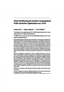
Figure 7: Different Data Distributions for d = 3, n = 10M , N = 20, BBS and real data. The distribution of the synthetic data is uniform, anticorrelated and correlated, as described in [2]. We vary the dimensionality from 3 to 7, while the cardinality of the dataset ranges from 1M-10M points. We also evaluate the effectiveness of the proposed partitioning approach using real-life data. We conducted experiments on a dataset containing information about real estate all over the United States, such as estimated price, number of rooms and living area (available from www.zillow.com). We obtained a 5dimensional dataset containing more than 2M entries. The dataset contains 5 attributes namely number of bathrooms, number of bedrooms, living area, price and lot area. Each experimental setup is repeated 10 times and we report the average values. The block size is set to 8K and the buffer size is 100 blocks. We used the same dynamic partitioning algorithm for grid and angle-based partitioning. All times are measured in msec. In all charts where it is applicable, we depict also error bars showing the deviation among the 10 different runs of the experiments, but in most cases the error bars are not visible since the deviation values are not significant.

7.1 Data Distribution Study In the first experiment, we compare the three partitioning techniques (random, grid and angle-based) using the BBS algorithm for skyline computation. We study a 3d dataset of n = 106 data points that follow different data distributions. The number of partitions is set to N = 20. Figure 7 shows the results in logarithmic scale. Based on Figure 7(a) we conclude that for all data distributions considered, the response time of the skyline query processing is significantly reduced when the angle-based partitioning is used. In particular using angle-based partitioning, we compute the skyline query from 2 up to 20 times faster than the execution based on grid partitioning. It is worth noting that for the correlated dataset, the random partitioning is comparable to the angle-based partitioning. This is because the random partitioning scheme maintains the initial data distribution in all partitions. In the case of correlated data, this leads to a sufficient performance of random partitioning. However, correlated data is not very challenging for skyline computation since the skyline cardinality is relative

small and this also leads to small response times in general. In addition, correlated data are not very interesting for skyline computation, since the skyline operator aims to balance contradicting criteria, as in the case of anticorrelated data. For uniform and more importantly anticorrelated datasets, which are deemed as hard problems for skyline computation, angle based partitioning outperforms random by one order of magnitude and grid partitioning by more than half an order of magnitude. In Figure 7(b) we study the average number of comparisons needed for the local skyline computation in terms of candidates examined for domination, which is a typical cost metric for BBS. It is expected that the correlated dataset requires the fewest domination tests but this advantage is not shown for the grid partitioning. Clearly, the angle-based partitioning requires less objects to be examined for domination. This indicates the higher pruning power of local skylines of the angle-based partitioning. This is also confirmed in Figure 7(c), which depicts the total number of local skyline points. The angle-based partitioning technique produces less local skylines for any data distribution and this improves the overall performance of the parallel skyline computation. Thereafter, we study in more detail the local skyline points and more specific the local skyline points that belong also to the global result set. We define the number of globallocal skylines of a partition i as the cardinality of the set  SKYPi SKYP . Figure 7(d) depicts the maximum and the minimum value of global-local skyline points retrieved by any partition for the anticorrelated dataset that produces the most skyline points. We also depict the deviation between the global-local skyline points retrieved by any partition. Note that for the random partitioning, all partitions have a similar number of global-local skylines, so that the minimum and maximum values have a relative small difference and the deviation is low. As expected, the grid partitioning has very high maximum value (for the partition including the origin of the space), but also a very low minimum value indicating that some partitions contribute only marginally to the result. Our angle-based partitioning has a quite balanced number of global local skylines and both maximum and minimum values are quite high.

15000 10000 5000 0

Random Grid Angle

15000

120

10000

80 60

20 0

2

4

6

8

0

10

0

2

4

5000

8000 6000 4000 2000 0

2

4

6

0

10

0

2

4

8

10

250

2000 1000

10

8

10

Random Grid Angle

200 150 100 50

0

2

cardinality

(d) Average comparisons

300

3000

0

8

(c) Average I/O

Random Grid Angle

4000

6 cardinality

max. local skylines

total local skylines

Random Grid Angle

10000

8

(b) Max. partition time

14000 12000

6 cardinality

(a) Response time

avg. comparisons

100

40

5000

cardinality

0

Random Grid Angle

140

avg. I/O

max. partition time

response time

20000

160

20000

Random Grid Angle

25000

4

6

8

cardinality

(e) Total local skylines

10

0

0

2

4

6 cardinality

(f) Max. local skylines

Figure 8: Scalability with cardinality: ANTICOR, d = 3 N = 20 n = {1M, 5M, 10M }, N = 20, BBS For the next figure, we define the metric compactness as  |SKYPi SKYP | ). The comcompactness = 100 ∗ avg1≤i≤N ( |SKYPi | pactness expresses how many points of the local result set of a partition, belong also to the global result set. In the best case scenario, all data points that do not belong to the global skyline set, would be discarded during local skyline computation. Therefore, high values of compactness indicate that the local result sets are more compact and contain less redundant data points. In Figure 7(e) the compactness for the three synthetic datasets is depicted. Notice that the compactness of the angle-based partitioning is quite high, which indicates how suitable the angle-based partitioning for skyline computation is. Note that for the uniform dataset, random and grid partitioning have similar values of compactness, since both maintain the initial data distribution. On the other hand, angle-based partitioning has a higher value of compactness, since it alters the data distribution on each partition. For the anticorrelated dataset all partitioning approaches achieve higher values of compactness, while for the correlated data distribution all partitioning methods achieve very low compactness values. The cardinality of the global skyline set differs depending the data distribution. For example, skyline points of a correlated dataset are only few and this leads to smaller values of compactness.

7.2 Scalability with Cardinality Next we evaluate the performance of the angle-based partitioning for datasets of different cardinality. In this experiment the dimensionality of the dataset is 3 while we vary cardinality between 1M and 10M. In this experiment we use an anticorrelated dataset. All charts in Figure 8 depict error bars showing the deviation among the 10 different runs of the experiments. Notice that the deviation values are not significant.

Figure 8(a) illustrates the response time for various dataset cardinalities. Angle-based partitioning outperforms both alternatives in all setups. As the cardinality increases the angle-based partitioning technique shows a more stable performance and the benefit increases. For n = 10M the anglebased partitioning performs 3 times better than the grid in terms of response time. We also depict the maximum time (Figure 8(b)), the average I/O (Figure 8(c)) and the average comparisons (Figure 8(d)) of all partitions, which influence partially the response time. Notice that the cardinality of the dataset influences in similar way all measures depicted in the charts. For example in the case of the average comparisons that indicate the pruning ability of each partition, angle-based partitioning requires 10 times less comparisons than random partitioning and up to 7 times less compared to grid partitioning. Figure 8(e) depicts the total local skylines and clearly shows that angle-based partitioning always results in smaller intermediate result sets, indicating its efficiency and guaranteing smaller transfer and merging costs. It is obvious that angle-based partitioning outperforms grid partitioning by means of local skyline points up to 10 times. Random partitioning performs even worse. Figure 8(f) shows the maximum number of local skyline points retrieved by all partitions. This influences mainly the transfer delay, and once again the gain of angle-based partitioning is obvious.

7.3 Scalability with Dimensionality In the next series of experiments we examine the proposed partitioning method’s scaling features with regards to the dimensionality of the dataset. We generate different datasets and increase the dimensionality from 3 to 7. For this experiment the settings are uniform dataset, n = 10M , N = 20 and SFS algorithm. In Figure 9 the performance of anglebased partitioning is compared against grid partitioning.

100

80

80

improvement (%)

response time

100

150000 100000

compactness

Random Grid Angle

200000

60 avg. comparisons 40 local total skylines merge comparisons 20

50000

1 5

10

20

30

40

0

50

Random Grid Angle

60 40 20

10

20

partitions

30

40

50

0

10

20

partitions

(a) Response time

(b) Improvement percentage over grid

30

40

50

partitions

(c) Percentage of global skylines

Figure 10: Number of Partitions: ANTICOR, d = 5, N = 10 − 50, n = 10M , SFS

80

improvement (%)

improvement (%)

80

60 50 40 30 20

60 40 total local skylines avg comparisons merge comparisons

20

10 0

7.4 Number of Partitions

100

Response Time Max Partition Time

70

3

4

5 dimension

6

7

0

3

4

5 dimension

6

7

(a) Improvement (%) over (b) Improvement (%) over grid in terms of time grid in various metrics Figure 9: Scalability with dimensionality

Figure 9(a) shows the improvement percentage in terms of time (defined as 100 ∗ GRID−ANGLE ). The response time GRID refers to the time passed from the time the query was posed till the results are computed at the coordinator. The maximum partition time refers to the CPU time needed for the local skyline computation by the slowest server. The improvement percentage of the response and the maximum partition time increases with the dimensionality. We notice that only for small values of dimensionality the improvement of the response time is larger than that of the maximum partition time. This is mainly, because the cardinality of the skyline set increases with the dimensionality and we have to transfer at least the global skyline points. In Figure 9(b) we depict the improvement percentage as far as number of comparisons and number of local skylines are concerned. The benefit of using the angle-based partitioning in terms of (average) comparisons per partition increases as the dimensionality increases. The smaller number of comparisons indicates the higher pruning power of anglebased partitioning. On the other hand, we notice that the improvement percentage for the total number of the local skylines decreases as the dimensionality increases. This is mainly due to the fact that the average cardinality of each partition does not change, but the dimensionality increases. Therefore, the percentage of points that are skyline points increases which in turn reduces the upper limit for the improvement percentage. Figure 9(b) also shows the improvement over grid in terms of merging comparisons. We notice that even though the number of elements that have to be merged, i.e. total local skylines, are much smaller for the angle-based partitioning, the gain in terms of merge comparisons is negligible. This is because most points returned by the angle-based partitioning are global skyline points.

In the next experiment, we study how different number of partitions affect the performance of the angle-based partitioning. In this experiment we use the anticorrelated data distribution and the SFS algorithm. The plot in Figure 10(a) illustrates the total response time taking into account the network delay. In all cases angle-based partitioning constantly outperforms the other two alternatives, namely grid and random partitioning. Figure 10(b) depicts the number of required comparisons for the parallel skyline computation, since the comparisons influence the processing time. We compare the number of comparisons required by the angle and grid partitioning, since the random partitioning performance is even worse than grid. As depicted in 10(b), the number of local skylines is improved more than 60% for all tested number of partitions. The small number of local skylines, influences the overall performance since it affects the merging phase, the data transfer cost and the number of comparisons for the local skyline computation. As far as the average number of comparisons is concerned, the angle-based partitioning executes up to 90% less comparisons, which clearly states that the angle-based partitioning technique is more suitable for skyline computation. The small number of required comparisons show the high pruning power of angle-based partitioning. The number of comparisons needed for merging does not improve significantly, because even though the input of the merging phase is much smaller, most of them are global skyline points, while the grid partitioning returns a lot of points that can be pruned immediately with only one comparison. We also notice that the improvement in terms of local skyline points increases with the number of partitions because there are more partitions with smaller cardinality which leads to even more local skylines produced by the grid partitioning. In Figure 10(c) the compactness for the different values of partitions is depicted. The compactness for all partitioning approaches falls while the number of partitions increase. This is mainly because the number of local skylines per partition does not significantly decrease while the partitions increase. Therefore, the global skylines are distributed over more partitions and the number of local skylines per partition does not decrease significantly, leading to lower values of compactness. Still angle-based partitioning manages to obtain high compactness values even for 50 partitions, which shows that it is scalable in terms of number of servers available. Finally, in Figure 11, we study the effect of increasing

total local skylines merge comparisons avg. comparisons

95

2000

improvement (%)

response time

100

Random Grid Angle

2500

1500 1000 500

90 85

[7]

80 75 70 65

10

20

30

40

partitions

(a) Response time

50

60

10

20

30

40

50

partitions

Figure 11: Real dataset, SFS algorithm. the number of partitions for the real dataset. The results show that angle-based partitioning achieves lower response times than the other approaches (Figure 11(a)), since it improves the average number of comparisons by 70-80% over grid (Figure 11(b)). This improvement is observed also in the number of total local skylines and at the merge comparisons respectively.

8.

CONCLUSIONS

In this paper we present a novel approach to partition a dataset over a given number of servers in order to support efficient skyline query processing in a parallel manner. Capitalizing on hyperspherical coordinates, our novel partitioning scheme alleviates most of the problems of traditional grid partitioning techniques, thus managing to reduce the response time and share the computational workload more fairly. As demonstrated by our experimental study, we are up to 10 times better than grid in terms of response time and constantly outperform both grid and random partitioning, thus becoming an efficient and scalable solution for skyline query processing in parallel environments. In our future work, we aim to examine the performance of angle-partitioning for subspace skyline queries. The novel angle-partitioning is not affected by the projection of the data points, during subspace skyline queries, since again the region near the origin is equally spread to all partitions.

9.

[8]

(b) Improvement (%) over grid [9]

[10]

[11]

[12]

[13]

[14]

[15]

[16]

REFERENCES

[1] W.-T. Balke, U. G¨ untzer, and J. X. Zheng. Efficient distributed skylining for web information systems. In Proc. of Int. Conf. on Extending Database Technology (EDBT), pages 256–273, 2004. [2] S. B¨ orzs¨ onyi, D. Kossmann, and K. Stocker. The skyline operator. In Proc. of Int. Conf. on Data Engineering (ICDE), pages 421–430, 2001. [3] S. Chaudhuri, N. N. Dalvi, and R. Kaushik. Robust cardinality and cost estimation for skyline operator. In Proc. of Int. Conf. on Data Engineering (ICDE), page 64, 2006. [4] J. Chomicki, P. Godfrey, J. Gryz, and D. Liang. Skyline with presorting. In Proc. of Int. Conf. on Data Engineering (ICDE), pages 717–719, 2003. [5] A. Cosgaya-Lozano, A. Rau-Chaplin, and N. Zeh. Parallel computation of skyline queries. In Proc. of Int. Symp. on High Performance Computing Systems and Applications, page 12, 2007. [6] Y. Gao, G. Chen, L. Chen, and C. Chen. Parallelizing progressive computation for skyline queries in

[17]

[18]

[19]

[20]

[21]

multi-disk environment. In Proc. Int. Conf. of Database and Expert Systems Applications (DEXA), pages 697–706, 2006. K. Hose, C. Lemke, and K.-U. Sattler. Processing relaxed skylines in PDMS using distributed data summaries. In Proc. of Conf. on Information and Knowledge Management(CIKM), pages 425–434, 2006. Z. Huang, C. S. J. H. Lu, and B. C. Ooi. Skyline queries against mobile lightweight devices in MANETs. In Proc. of Int. Conf. on Data Engineering (ICDE), page 66, 2006. H. V. Jagadish, B. C. Ooi, and Q. H. Vu. BATON: A balanced tree structure for peer-to-peer networks. In Proc. of Int. Conf. on Very Large Data Bases (VLDB), pages 661–672, 2005. D. Kossmann, F. Ramsak, and S. Rost. Shooting stars in the sky: An online algorithm for skyline queries. In Proc. of Int. Conf. on Very Large Data Bases (VLDB), pages 275–286, 2002. H. Li, Q. Tan, and W.-C. Lee. Efficient progressive processing of skyline queries in peer-to-peer systems. In Proc. of Int. Conf. InfoScale, page 26, 2006. E. Lo, K. Y. Yip, K.-I. Lin, and D. W. Cheung. Progressive skylining over web-accessible databases. Data & Knowledge Engineering, 57(2):122–147, 2006. J. Nievergelt, H. Hinterberger, and K. C. Sevcik. The grid file: An adaptable, symmetric multikey file structure. ACM Transactions on Database Systems (TODS), 9(1):38–71, 1984. D. Papadias, Y. Tao, G. Fu, and B. Seeger. Progressive skyline computation in database systems. ACM Transactions on Database Systems (TODS), 30(1):41–82, 2005. S. Ratnasamy, P. Francis, M. Handley, R. Karp, and S. Schenker. A scalable content-addressable network. In Proc. of Int. Conf. on Applications, Technologies, Architectures, and Protocols For Computer Communications (SIGCOMM), pages 161–172, 2001. J. T. Robinson. The K-D-B-tree: a search structure for large multidimensional dynamic indexes. In Proc. of Int. Conf. on Management of Data (SIGMOD), pages 10–18, 1981. K.-L. Tan, P.-K. Eng, and B. C. Ooi. Efficient progressive skyline computation. In Proc. of Conf. on Very Large Data Bases (VLDB), pages 301–310, 2001. A. Vlachou, C. Doulkeridis, Y. Kotidis, and M. Vazirgiannis. SKYPEER: Efficient subspace skyline computation over distributed data. In Proc. of Conf. on Data Engineering (ICDE), pages 416–425, 2007. S. Wang, B. C. Ooi, A. K. H. Tung, and L. Xu. Efficient skyline query processing on peer-to-peer networks. In Proc. of Int. Conf. on Data Engineering (ICDE), pages 1126–1135, 2007. R. Weber, H.-J. Schek, and S. Blott. A quantitative analysis and performance study for similarity-search methods in high-dimensional spaces. In Proc. of Int. Conf. on Very Large Data Bases, pages 194–205, 1998. P. Wu, C. Zhang, Y. Feng, B. Y. Zhao, D. Agrawal, and A. E. Abbadi. Parallelizing skyline queries for scalable distribution. In Proc. of Conf. on Extending Database Technology (EDBT), pages 112–130, 2006.