Cylindrical Space Partitioning for Ray-Tracing

Cylindrical Space Partitioning for Ray-Tracing Gilles Subrenat, Christophe Schlick

LaBRI 1 351 cours de la Liberation 33405 Talence (FRANCE)

[subrenat|schlick]@labri.u-bordeaux.fr

Abstract: In this paper, we present a new space partitioning scheme for ray tracing based algorithms which divides a given region of the scene into cylindrical slices. Our rst motivation was to nd a four-connected partitioning scheme that is ecient for the parallel architecture we use for our parallel rendering environment [7], but the technique is interesting by itself and may be useful in sequential environments as well. The new partitioning scheme can be seen as an intermediate solution between rectangular grids [5] and spherical pyramids [15].

Keywords: Computer Graphics, Ray Tracing, Optimization, Space Partitioning

1 Introduction It is well-known that in every rendering algorithm using a ray tracing basis (classical ray tracing [17] [3] or ray tracing based radiosity [16] [13]), a large part of the computation time is spent in the calculation of potential or actual intersections between rays and objects in the scene. In the last decade, numerous optimization techniques have been proposed (bounding volumes [17] [12], slabs [11], octrees [6], grids [5], macro-regions [4], ve-dimensional subdivisions [1], pyramids [15], hybrid decompositions [14]) to reduce the number of unneeded intersection computations. This paper presents a new space partitioning scheme for ray tracing based algorithms which divides a given region of the scene into cylindrical slices. The new partitioning scheme can be seen as an intermediate solution between rectangular grids [5] and spherical pyramids [15]. The three techniques are compared both qualitatively and quantitatively. As the grids and the pyramids, the new partitioning scheme can be applied once to the whole scene but a better solution would be to use it as a leaf node in a hybrid hierarchical decomposition [14]. In Section 2 we recall shortly some existing partitioning methods. In Section 3 we detail our implementation of the pyramidal partitioning technique. In Section 4 we present the new method. Finally, in Section 5 we discuss and compare the eciency of grids, pyramids and cylindrical slices on several aspects.

2 Space Partitioning Techniques The main purpose of every space partitioning technique is to decrease the number of intersection computations by searching for the most probable ones. The principle is to divide the space into regions, and then, to associate a list of objects to each of them. Thus, if a ray does not cross a region, there is no need to compute the intersection with any object inside. On the other hand, this partitioning implies some overcost both in computation time (to associate each object with the right region(s) and to nd the regions crossed by a given ray) and in memory space (to store the list of objects for each region). Therefore, some tradeo has to be made. Unfortunately, nding the optimal partitioning for a given scene is almost impossible because of the large number of parameters that are involved. Laboratoire Bordelais de Recherche en Informatique. Universite Bordeaux I et CNRS URA 1304. The present work is also granted by the Conseil Regional d'Aquitaine. 1

1

All the partitioning techniques that have been proposed in the literature can be divided in three main families:

Object Dependent Space Partitioning: In the rst family, regions directly surround the ob-

jects and therefore are strongly related to the position or orientation of the objects. These surrounding regions (called bounding volumes) have usually simple shapes which allow ecient ray-region intersections: spheres, parallelepipeds [17], slabs (pairs of parallel planes) [11]. To reduce the number of ray-region intersections, bounding volumes can be grouped into a tree structure [12]. Scene Dependent Space Partitioning: In the second family, regions are computed more or less independently from the position and orientation of the objects. More precisely, the whole scene is subdivided either uniformly by rectangular grids [5] or spherical pyramids [15], or adaptatively by octrees [6], non-uniform grids [10] or macro-regions [4]. Note that a vedimensional partitioning has also been proposed [1] in which the scene is subdivided according to the three axis de ning a position and the two angles de ning a direction. Nevertheless this technique is somehow dierent from the others because it creates overlapping regions. Hybrid Space Partitioning: The last family tries to get the best of both worlds by combining object dependent and scene dependent partitionings. For instance, in [14] a hierarchical decomposition is used which combines parallelepipedic bounding boxes and grids. This technique has become very popular and is proposed in almost every commercial or even public-domain ray tracer. The reason for this popularity is that the optimization works well for a large range of scenes, whether the objects are uniformly or unevenly distributed. As a counter part, one major drawback of hybrid partitioning is that an ecient hierarchical decomposition can hardly be found automatically and has usually to be provided by hand. Nevertheless, if the superiority of hybrid partitioning has been clearly established, an interesting research direction could be to nd some alternatives to the grids for the leaves of the hierarchical decomposition structure. In the next sections, we propose to study the possibilities of pyramids or cylindrical slices as such alternatives.

3 Pyramidal Space Partitioning 3.1 Principle The basic idea of pyramidal space partitioning, introduced by Speer [15], is to cut the scene, not according to the possible positions (three degrees of freedom: x, y and z ), but according to the possible directions (two degrees of freedom:  and '). Therefore this process can be seen as a simpli cation of [1] where the space subdivision is done only in two dimensions rather than ve. But, since the regions are not overlapping (as they are in [1]), the process should better be considered as a replacement of the grid. The initial step in the pyramidal partitioning process is to choose the central point O of the subdivision and the central axis which becomes the vertical axis Oz of the new frame. The rst subdivision is performed according to the azimuthal angle  by moving a vertical half-plane regularly around the central axis (Figure 1a) which is equivalent to cut a sphere into longitudes. Each region obtained by this step is named a slice. Then, each slice is regularly cut from top to bottom according to the zenithal angle ' (Figure 1b) which is equivalent to cut a sphere into latitudes. Each region obtained here is simply named a pyramid (see Figure 1c for a 3D view). Regular subdivision means that each pyramid has the same volume than the others. In the original paper, pyramids were essentially employed as a global structure in which the whole scene is partitioned. We think this approach is not sucient because it is not adapted to scenes with uneven object distribution. A better use of pyramidal partitioning should be to consider it as an alternative to the grid for the leaves of the hierarchical partitioning [14]. 2

12 longitudes

4 latitudes

A O

A a) Top view (subdivision in θ)

b) Side view along A-A (subdivision inϕ)

c) 3D view

Figure 1: Pyramidal space partitioning

3.2 Properties In comparison with other partitioning schemes, the pyramidal space partitioning technique includes some characteristics which seem attractive and have motivated our work on the subject. First of all, thanks to its spherical symmetry, this partitioning is independent of any orientation of the scene according to the absolute frame. With a partitioning strongly related to the primary directions of the frame (grid, octree, etc), Hall has noticed [9] that a factor 10 may exist for computation time of a same scene, when objects are parallel to the axis or rotated by 45 degrees. Such a property is particularly interesting for animation. Another advantage is that the partitioning is done in two dimensions rather than in three, so we may hope less computation. Such a property is interesting for a parallel implementation on distributed memory computers (one of our purposes) because of the strongly four-connected aspect of most communication networks (T.Node, Paragon or other). Finally, as will be detailed in Section 3.5, this technique allows to sort the objects that belong to a pyramid. Therefore, it corrects one default of classical partitionings noticed by several authors: when a ray enters a region, the intersections with all objects of the region must be computed because there is no order (even partial) inside the region that would enable to stop computation before all intersections have been tested. Since the pyramidal partitioning technique is not widely known and since several implementation aspects have not been fully explained in [15], we are going to detail our implementation for data distribution and ray progression.

3.3 Data Distribution It is not always very easy to determine on which side of a plane an object lays, and it may be very costly anyway. In our implementation, we are working with the bounding boxes of objects: we must nd which pyramids include a bounding parallelepiped oriented along the coordinate axis. The most trivial case happens when the central point is inside the bounding box, the object is then inserted in all pyramids. For the other cases (the most numerous ones), data distribution is done in two steps: rst the slices including the object are computed and then, for each elected slice, the pyramids containing the object are established. The data distribution in slices is done in the following way: if the central axis intersects the bounding box, the object is inserted in all slices (Figure 2a). Otherwise the object is inserted according to the x and y coordinates of its bounding box. More precisely, we compute the slices which contain the four points (xmin ,ymin), (xmax ,ymin ), (xmin ,ymax ) and (xmax ,ymax ), we determine the two extremal slices and all slices between them are selected (Figure 2b). For each slice including an object, the data distribution in pyramids is done in a similar way: if 3

Top view ( θ) 3

2

1

Side view ( ϕ) 3

4

2

1

0

1

0

1

4

5

0

5

0

6

11

6

11

7

10 8

7

9

2

3

10 8

(a) All slices

2 3

4

9

5

(b) Slices 0 to 2

(c) Pyramids 0 to 3

4 5 (d) All pyramids

Figure 2: Object repartition into pyramids the upper and lower vertical planes cross the bounding box, the object is inserted in all pyramids (Figure 2d). Otherwise, we compute the pyramids which contain the eight vertices of the bounding box and select pyramids between the two extremal ones (Figure 2c).

3.4 Ray Progression The ray progression begins by computing the pyramid in which the ray starts and the plane which it crosses rst (four ray-plane intersections are needed, one for each side of the pyramid). Then, during the progression, three ray-plane intersections are necessary each time the ray crosses a pyramid. A computation of an intersection between a ray and a plane needs seven additions and seven multiplications. So each progression step requires three comparisons, twenty-one additions and twenty-one multiplications. Obviously, this appears very expensive compared to the incremental progression in a rectangular grid, but an interesting property of pyramidal space partitioning is that a ray will be trapped in a pyramid after some crossings, and so we can generally expect few crossings. However, we will see in Section 5 that a trapped ray may rise some other problems about the computation cost.

3.5 Object Sorting If we x the number of subdivisions N in a given dimension, there will be N 3 regions for the grid but only N 2 for pyramids. It means that a pyramid is N time larger than a voxel, and so contains in average N times more objects which may be intersected. This counteracts the desired optimization. On the other hand, for each object, one can compute its minimal and maximal distances with regard to the central point: this induces the possibility to sort objects in a pyramid according to this distance criterion. This sorting can be used as follows [15]: First, according to the incoming and outgoing points of the ray, its in uence zone in the current pyramid is computed (Figure 3a). All objects that are included, either partially or totally, in that zone are potential clients. On the Figure 3a, objects 1 and 2 are retained for a potential intersection, while object 3 is automatically discarded. Now, look at Figure 3b, we can see that the above optimization is inecient because the in uence zone is extended on the whole pyramid. To solve this problem, we use the sorting provided by the pyramid. In Figure 3b, we begin computation with object 1 (the rst one in the sorted list), we nd an intersection and see that object 2 is beyond the intersection point (i.e. the minimal distance between object 2 and central point is greater than the distance between the intersection point and the central point), so there is no need to compute an intersection with object 2. Note that this process can also be applied in Figure 3a: if object 1 is intersected, there is no need to compute an eventual intersection with object 2 because it would be beyond the rst one.

4

2

Ray 2

3 1 Min

1 Ray Max (a) Influence area

(b) Sorted objects

Figure 3: Pyramids and intersections Top view

Side view along A-A

A O

A Latitudes ( ϕ)

Longitudes ( θ)

Figure 4: Addition of a central cylinder to avoid round-o errors

3.6 Prevention of Round-o Errors The zone surrounding the central axis (and more particularly the central point) is very sensitive to round-o errors. A high number of partitioning regions share this line, and when a ray comes close to this axis, round-o errors may produce unpredictable behaviors. This problem was not mentioned in the original paper [15] but it has to be solved because it creates visible artefacts (some pixels are incorrectly colored) or even in nite computation loops. We propose a simple solution in which the central axis is surrounded with a cylinder (Figure 4). When a ray enters this cylinder, the notion of pyramid is forgotten, to reappear when the ray leaves the cylinder. A ray-cylinder intersection involves a quadratic equation but this equation is seldomly solved because many rays do not hit the cylinder and so the resolution is stopped before the square root. Anyway, the cylinder may also be replaced by its parallelepipedic bounding box which provides the same features.

4 Cylindrical Space Partitioning If we compare the advantages and the drawbacks of the grid and the pyramids, they appear almost perfectly antagonistic. Indeed, the grid allows fast data distribution and ray progression but is strongly dependent of the coordinate axis and does not enable any object sorting in the voxels. On the other hand, a pyramidal partitioning does not have any privileged direction and oers the possibility to sort the objects inside a pyramid, but involves expensive algorithms for the data distribution and the ray progression. If you consider grid as a partitioning scheme in cartesian coordinates, pyramids as a partitioning scheme in spherical coordinates, it is quite natural to think about a partition scheme in cylindrical 5

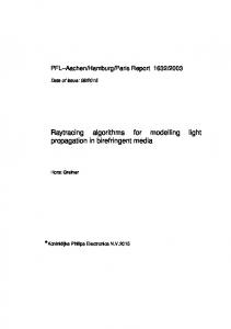
12 longitudes

4 altitudes

A O

A a) Top view (subdivision in θ)

b) Side view along A-A (subdivision in z)

c) 3D view

Figure 5: Cylindrical space partitioning coordinates.

4.1 Principle The basic idea is to cut the scene with an horizontal subdivision done according to the possible directions (one degree of freedom: ) and a vertical subdivision done according to the possible positions (one degree of freedom: z ). Therefore the process can be considered as an intermediate solution between grids and pyramids. The rst step of the cylindrical partitioning process is to choose the central axis, which becomes the vertical axis Oz of the new frame. The rst subdivision is then performed according to the azimuthal angle  in the same way as for the pyramids (Figure 5a). Each region obtained by this step is also named a slice. Then, each slice is regularly cut from top to bottom with horizontal planes (Figure 5b). Each region obtained here is named a piece of cake, or a cake for short (see Figure 5c for a 3D view). Note that in the actual implementation a central cylinder should be added, as we have proposed for the pyramids, in order to avoid round-o errors.

4.2 Data Distribution The data distribution in horizontal slabs is trivial and, for a given object, it can be computed once for all slices. The data distribution in slices is done exactly in the same manner as with pyramids. The computation time required by this step is essentially proportionate to the number of slices (N ) and not to the number of cakes (N 2 ). This cost is always higher than for the grid but much lower than for the pyramids.

4.3 Ray Progression The rst step is to compute in which cake the ray starts as well as the ray direction according to  and to z . The progression through horizontal slabs is incremental as in a grid, the cost for one traversal is two comparisons and two additions. On the other hand, the progression through slices requires the computation of a ray-plane intersection (seven additions and seven multiplications). To sum up, as for the data distribution, the cost of one traversal is always higher than for the grid but much lower than for pyramids (three ray-plane intersections). One property of pyramids is not preserved by cakes: a ray can not be trapped anymore (except for pure horizontal rays). But in Section 5, we will show (contrarily to [15]) that ray trapping is in fact a drawback rather than an advantage.

6

processor boundaries

Z

internal subdivisions

Y

X

Figure 6: Scene partitioning among dierent processors

4.4 Object Sorting The same principle as with pyramids is used, except that the distances are not computed relative to the central point but relative to the central axis.

5 Results 5.1 Number of Ray Progressions In a ray tracing based algorithm implemented on a sequential architecture, the number of ray progressions is not a relevant criterion because its cost is negligible compared to other parts of the computation (ray-object intersection, shading, texturing, etc). But if you take a parallel architecture, things are dierent. Indeed, a way to parallelize a rendering algorithm based on a ray tracing scheme is to cut the scene into regions and to aect each region to a given processor [7]. Therefore, when a ray travels from one region to another, it implies some communication between the two corresponding processors. Parallel computers have often four-connected communication networks (Paragon, T.Node, etc) thus it may be necessary to obtain a two-dimensional subdivision of the scene in order to optimize communication between processors. Pyramids and cakes are naturally suited to a four-connected implementation, but the grid can also be easily adapted by suppressing a direction of the subdivision. It means to cut the scene into N  N  1 (or N  1  N or 1  N  N ) voxels (see Figure 6). Once the scene is shared among processors, it is possible (and advisable) to have an internal partitioning inside each region to speed up computation into it. Therefore, the missing dimension of the grid can be easily restored internally (Figure 6). To study the in uence of the three partitioning schemes on the number of ray crossings, we have created a test scene which is simply an empty cube. We traced 1 419 857 rays (173 points of departures and 172 directions for each origin) for each type of partitioning. The purpose was to compare performances with the same number of processors, so we took N N 1 voxels for the grid, N  N cakes and N  N pyramids, where N takes dierent values2 between 7 and 140. For each measure, we have counted the number of crossings from one region to another (Table 1). Pyramids and cakes exhibit the same behavior (there is less than 1% dierence). A priori, pyramids should behave better because they are able to trap rays; but this property is ful lled only for a large distance from the central point and therefore the ray has usually left the bounding volume of the scene before it arises.

2 100 or 140 subdivisions in each dimension may appear excessive, but in a parallel environment, scenes are usually very complex and such a size may be justi ed.

7

N = Size Type of partitioning of the Grid Grid Cakes Pyramids subdivision (N  N  N ) (N  N  1) (N  N ) (N  N ) 7 5 939 475 3 959 283 3 190 579 3 312 394 10 8 699 178 5 817 454 4 573 413 4 685 595 17 15 485 430 10 349 736 7 915 027 8 036 381 24 22 097 481 14 777 171 11 427 905 11 461 625 41 38 470 468 25 726 774 19 691 065 19 620 816 58 54 604 268 36 516 888 27 931 863 27 758 948 99 93 921 179 62 810 501 47 810 141 47 423 643 140 132 988 985 88 936 801 67 775 020 67 083 611 Ratio + 100% +30% +0%  increase of the number of crossings in comparison with pyramids Table 1: Number of crossings between regions

N = Size Type of partitioning of the Grid Cakes Pyramids subdivision (N  N  N ) (N  N ) (N  N ) 7 1 18 42 17 2 20 240 41 4 34 429 58 6 45 833 99 7 74 2678 Table 2: Data distribution times (seconds) A N N 1 grid produces thirty percent more crossings than for pyramids and cakes and a N N N grid doubles the number of crossings. One can notice that this behavior is also veri ed in a non-empty scene.

5.2 Data Distribution Our test scene (Figure 8) is a cube containing ve Sirpinski tetrahedrons [8] made of 4096 triangular facets each (which means about 20 000 facets). We have measured the time spent to distribute data among regions for each type of partitioning. Table 2 shows results for dierent subdivision sizes. For the grid, the distribution times are negligible whatever the size of the grid. For cakes, the timings are larger but remain reasonable (there is more or less a constant factor 10 between the grid and the cakes). On the other hand, pyramids have a behavior that deteriorates quickly with an exponential factor. For N = 99, time is really a problem for a scene that is not very complex.

5.3 Number of Intersections and Computation Time Using the same scene as above, we trace a total of 135 rays from several points of departures and towards several directions. This time, we measure the number of intersections as well as the total computation time needed to treat all rays (Table 3). In all cases, the grid requires less computation time than the two other partitionings, even if it involves more intersection computations. The main reason is that the primitives used here (triangular facets) are very simple. For cakes, the crossing of a ray from one region to another involves an intersection with a plane which has almost the same complexity as for an intersection with a facet. For instance, when N = 24, cakes require as many crossings as intersections which 8

N = Size of the subdivision 7 10 17 24 41 58 99

Type of partitioning Grid Cakes Pyramids (N  N  N ) (N  N ) (N  N ) 121 856 074 78 303 055 99 326 763 (757 s) (959 s) (1132 s) 61 691 750 42 195 767 59 850 991 (413 s) (604 s) (771 s) 24 919 790 15 731 699 24 656 777 (198 s) (311 s) (409 s) 11 822 923 10 962 709 15 305 318 (125 s) (275 s) (325 s) 5 802 691 5 083 592 8 356 284 (99 s) (218 s) (281 s) 4 081 419 3 980 718 6 731 789 (94 s) (235 s) (296 s) 2 610 143 3 535 231 6 272 990 (109 s) (299 s) (382 s)

Table 3: Number of intersections and computation time means twice more computations. If objects were more complex (quadrics, spline patches, implicit surfaces), these timings would have been reversed because the computation involved by the crossings would become negligible compared to the intersections.

5.4 Cakes vs. Pyramids The fact that pyramids take more time than cakes was foreseeable because of the overcost due to ray progression through pyramids. However, it is more surprising that pyramids compute more intersections than cakes (in a factor ranging from 1.2 to 2.0). That result can be explained if you notice that every ray that passes close to the central point may create excessive computation. Indeed, if it does not hit any object, the ray crosses the whole pyramid and computes intersections with all objects inside it. The same drawback holds for any trapped ray. On the other hand, cakes are statistically much more ecient. This problem is illustrated on Figure 7 which shows a side-view respectively for a pyramidal (left column) and a cylindrical (right column) partitioning. On each gure, the gray shaded part represents the zone of the scene for which potential intersections are computed for a given ray. One can see that pyramids have an uniform behavior whatever the value of angle  (Figures 7a and 7c). The ray must compute intersections with all objects inside the pyramid. On average, a ray must explore an area given by: (1) Area(Pyra) = N1 where N is the number of pyramids For cakes, two cases must be studied:  < =4 and  > =4. In the rst case (Figure 7b), the area to examine is always 1=N . In the second case (Figure 7d), the area to examine varies from 0 to 1=N , and on average, it is given by: for  > 4

Z 2 4 () d Area(Cake) =   N cos  sin () = 4 

9

(2)

1

Intersection zone Ray Pyramid boundaries Cake boundaries θ

θ 1

(a) ray caught in a pyramid

Global bounding box

(b) same ray as (a) in cakes

1

1

Area(a) = 0.20081 Area(b) = 0.20 Area(c) = 0.20081 θ

θ

Area(d) = 0.08

1

(c) ray caught in a pyramid

1

(d) same ray as (c) in cakes

Figure 7: Behavior of \central" rays By combining the two cases, we obtain:

ln2 + 1 Area(Cake) = N 2N which explains the dierence experimentally observed.



0:72 N

(3)

5.5 Grid vs. Cakes Up to N = 17, cakes behave better than grids which involve about 50% more intersection computations. From N = 24, performances decrease and for very large values of N , the grid performs better than cakes. Anyway for practical cases, such a large number of subdivisions for each dimension is seldomly used. Indeed, if you have a scene with a high level of complexity which requires a large number of regions for ecient optimization, the best solution is usually to create a hierarchical partitioning were the leaves are grids or cakes with a relatively small number of subdivisions.

6 Conclusion In this paper we have proposed a new space partitioning scheme for ray tracing based algorithms in which a given region of the scene is subdivided in cylindrical parts called cakes. This new technique can be considered as an intermediate solution between grids (where the subdivision is done in cartesian coordinates) and pyramids (where the subdivision is done in spherical coordinates). Thus it combines more or less the advantages of both partitioning techniques: like grids, it allows relatively fast data distribution (linear in the number of slices) and ray progression (one ray-plane intersection); and like pyramids, it is more or less independent of any direction and it enables to sort objects in each cake. Like grids and pyramids, cakes can be used either as a global partitioning structure for the whole scene or as the leaves of a hierarchical partitioning structure. According to our results, pyramids 10

Figure 8: Test scene seem to be less ecient, whereas grids and cakes are quite comparable. When looking at the number of traversals and the number of intersections, cakes behave better than grids, which makes them a candidate of choice for scenes with complex primitives (i.e. non-tessellated objects).

References [1] J.Arvo, D.Kirk, Fast Ray Tracing by Ray Classi cation, Proc. of SIGGRAPH '87, p55-64, 1987. [2] J.Cleary, B.Wyvill, Analysis of an Algorithm for Fast Ray Tracing using Uniform Space Subdivision, The Visual Computer, v4, p48-56, 1988. [3] R.Cook, T.Porter, L.Carpenter, Distributed Ray Tracing, Proc. of SIGGRAPH 84, p165-174, 1984. [4] O.Devillers, The Macro-Regions : An Ecient Space Subdivision Technique for Ray Tracing, Proc. of EUROGRAPHICS 89, p27-38, 1989. [5] A.Fuji, T.Tanaka, K.Iwata, ARTS : Accelerated Ray Tracing System, Computer Graphics and Applications, v6, n4, p16-26, 1986. [6] A.Glassner, Space Subdivision for Fast Ray Tracing, Computer Graphics and Applications, v4, n10, p15-22, 1984. [7] P.Guitton, J.Roman, G.Subrenat, A Parallel Method For Progressive Radiosity, Internal Report n.992-95, LaBRI, Universite Bordeaux 1, 1995. [8] E.A.Haines, A Proposal for Standard Graphics Environment, IEEE Computer Graphics & Applications, v7, n11, p3-5, 1987. [9] E.Haines, Comparison between Ray Tracers, Ray Tracing News (electronic newsletter), v3, 1990. [10] D.Jevans, B.Wyvill, Adaptive Voxels Subdivision for Ray Tracing, Graphics Interface'89, p164-172, 1989. [11] T.L.Kay, J.T.Kajiya, Ray Tracing Complex Scenes, Proc. of SIGGRAPH 86, p269-278, 1986. [12] S.Rubin, T.Whitted, A 3D Representation for Fast Rendering Complex Scenes, Proc. of SIGGRAPH 80, p110-116, 1980. [13] P.Shirley, Physically based Lighting Calculations for Computer Graphics, PhD thesis, University of Illinois, 1990. [14] J.Snyder, A.Barr, Ray Tracing Complex Models containing Surface Tessellations, Proc. of SIGGRAPH 87, p119-128, 1987. [15] L.R. Speer, A New Subdivision Method for High-Speed Memory-Ecient Ray-Shooting, Proc. of Third Eurographics Workshop on Rendering(Bristol, England), p45-59, 1992. [16] J.Wallace, K.Elmquist, E.Haines, A Ray Tracing Algorithm for Progressive Radiosity, Proc. of SIGGRAPH 89, p335-344, 1989. [17] T. Whitted, An Improved Illumination Model for Shaded Display, Comm. of the ACM, v23, n6, p343-349, 1980.

11