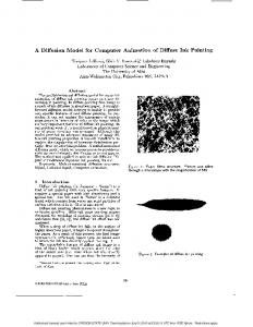
Rendering animations requires data structures which allow for ... an animation model based on an annotated graph, on de nitions of ... Computer animation lives from motion 25]. Pri- marily ...... Disney Animation: The Illusion of Life. Abbeyville ...
AniGraph | A Data Structure for Computer Animation Michael Braun, Arno Formella Computer Science Department University of the Saarland 66041 Saarbrucken, Germany
Abstract Rendering animations requires data structures which allow for an easy handling of the movements and changes in the scene. For a sophisticated renderer, it is very important to access the information describing the motion of the objects, because such knowledge can be used to reduce the render time. We describe an animation model based on an annotated graph, on de nitions of dimensions and on implementations of functions. The data structure with its simple interfaces provides an easy to use instrument to produce computer animations. On the one hand, the model is almost independent from a static modeler and a nal renderer, but on the other hand, it can be adapted easily to the needs of a speci c project. In the current implementation an artist needs to work closely together with a programmer.
1 Introduction Computer animation lives from motion [25]. Primarily, objects in a scene are moving around, but the actions are not restricted to geometrical changes. Almost all parameters such as shape, surface property, illumination etc. can be animated. Computer animation, which can be seen as an extension of classical computer graphics, was made possible over the last years with the availability of powerful machines [16, 28]. The time to render a single image|even in high resolution|could be reduced to a few minutes. Programmers and artists or animators worked together and generated arti cial worlds with their own laws and properties in such a way that they appear to be realistic although they might never be. Film production and advertising are using more and more computer animation as a basic tool for their special e�ects, which often is less expensive than the classical means and which allows for reproducible and modi able e�ects. Visualization of data gathered through simulations or measurements in the real world
becomes more and more important in many areas of science. The scientist wants to \see" what happens to the data or the models if some of the parameters are changed. Complex animations require to model the change over time of a possibly large set of parameters which in many cases are not independent of each other. Most animation systems generate lms frame by frame. For each frame a description of the frozen scene at the given time stamp is used as input data for the renderer. The method is similar to the traditional way to produce cartoons [14]. A more sophisticated renderer is able to render a set of frames faster, because the program re{uses information calculated for previous frames in the set [3, 10, 13, 18, 27], We restrict our animations to such cases that are entirely generated with a computer, i.e., the input data describe a set of objects with their properties which are to be displayed in an interval of time. We do not consider the classical means used in video technology or during the post production of a lm. The techniques such as key{framing, inbetweening, chroma{ keying, blending etc. can introduce some sort of animation too [7, 28]. They are still applicable for the nal tune up. We introduce in section 2 our animation model. The kernel of the model is an animation graph. The graph holds all functions and parameters which are animated. An evaluation strategy with a simple interface allows to extract the information needed to render a particular frame or a sequence of frames simultaneously. Our e�ort in implementing the system is described in section 3. Section 4 presents some example lms we have produced with the model. In section 5 we mention some extensions to the model we consider for a further development.
2 Animation Model At the beginning, we assume that the lm is generated frame by frame. The production of the lm
can be divided into four main parts. First, the scene containing all objects has to be designed. Second, the parameters that will be animated in the lm have to be separated from those remaining constant. Third, the values for the animated parameters have to be calculated at the time points for the frames. At last, the frames have to be rendered. An object can be anything that the renderer is able to visualize. The description of an object can be simply a set of data or for more complex objects a procedure generating the object. However, in every case an object appears as a set of variables|mostly just real numbers|that de ne the properties of the object. An animation of the object is given by assigning di�erent values to a subset of the variables [6, 8, 15, 17]. There exist di�erent ways to assign values to variables: explicitly by data sets, interactively by spline functions [5], functions curves [23] etc., or procedurally by simulations or iterations [11, 19]. In any way, they can be implemented as functions or procedures in a programming language with some well de ned interfaces. The more parameters are animated the more di�cult becomes the control of the interactions. It is almost impossible to animate a large set of objects that should behave realistically through an interactive system which allows just to use spline functions for each parameter. In many cases integration or di�erentiation is necessary to design an eloquent movement [1]. Dependencies between objects are often di�cult to handle and most systems provide only a xed set of tools to let certain types of objects interact with each other. Such tools include inverse kinematics [2, 9, 29], free form deformations [4, 21], actors [16] or particle systems [12, 24, 26]. In the sequel we introduce an animation model (see gure 1) that is able to integrate almost any tool describing dependencies between parameters and that provides the interface to evaluate those parameters at an arbitrary instant of time. Parameters of an animation will have types, which we call dimensions. Superposition and casting are two basic features of the de nition of a dimension. The de nitions are gathered in a dimension library (DLIB). The modi cation of animated parameters is performed by functions. Their de nitions are collected in a library too (FLIB). Such functions are implemented in a programming language, which provides the potentiality to design a large variety of basic \movements". A speci c animation is described in an animation graph which represents the interactions of the objects and which uses both the dimension library and the function library. An evaluation kernel that interprets
Scene (static)
Interface
Renderer
t f(t) evaluate
FLIB DLIB (libraries)
const
Figure 1: Animation model the graph is used by an interface to produce the required values for the parameters at a certain instant of time or over a certain period of time. The animation model is extendible by adding new functions or dimension types to the libraries. The interfaces to these libraries are clearly de ned (see section 3), so new methods to specify animations are easy to include into the system. An important property of the model is the fact that it is not possible to perform simulations (such as collision detection [20, 22]) or iterations directly with the graph. One has to provide the appropriate function libraries that do the calculation and that deliver the parameters to the system. However, once the parameters are generated they can be used to control the animation. For instance, a particle simulator including a collision calculation can be added as a base function which would deliver instants of time and all positions of the objects when collisions happen. The rest of the animation can react on these events, but the simulation itself can not be in uenced.
2.1 Time and Animation The basic parameter in an animation is the global time. In a nished lm everything happens at a speci c instant of time. However, while designing an animation it is often more convenient to assume local time frames with their own start and end points as well as durations. When all parts are modeled, the subanimations are combined. Formally, an animation is a function A : T ?! X1 � : : : � Xn where T is an ordered set, the global time, and Xi (i = 1; : : :; n) are arbitrary sets, the parameter sets
of the animation, representing possible values of the animated parameters. In the following T will be the set IR , so we can work with continuous animations. There exists always a global time during an animation. Nevertheless, we will be able to assign local times to di�erent parts of an animation as it is described later. The notion of the parameter sets becomes clearer with the de nition of dimensions.
2.2 Dimensions A movement of a parameter over time must be expressed within a coordinate system. The axes of such a system represent values of a certain type and are called dimensions. Superpositions are used to overlap in a natural way di�erent movements of an object in its dimensions. The idea provides the ability to specify what should happen if an object is animated with several functions at the same time. The concept allows for building more complex animations on the base of simple functions that can be overlapped or to arrange animations in hierarchies. We de ne a dimension type as (X; sup), where X is a set of values and sup is a function to calculate the superposition of values in that dimension, i.e., sup : X ?! X �
with the following two properties: (1) (2)
8x 2 X : sup(x) = x 8xi 2 X (i = 1; : : :; n) :
sup(x1 ; : : :; xn) = sup(x�(1) ; : : :; x�(n))
for all permutations �. Thus, superpositions preserve identity and are invariant to permutations of their parameters. Each set X contains an element ", the empty element, as the center of this dimension. Note that a dimension must not necessarily be ordered, so that the meaning of a center may not be intuitive. For x 2 X the superposition sup(x; ") = sup(x) = x computes the identity. We use the center as a mean to assign implicitly values to parameters. Examples of dimension types are (R I 3 ; +), where + is the common vector addition, or (Col; supRGB ), where PCol = [0 : 1]3 and supRGB (c1 ; : : :; cn) = n 1=n � i=1 ci is the average color. More abstract dimensions are e. g. (List; cat), where List represents unordered lists of items and cat is the function to concatenate several lists, or (Event; next), where Event
is a sequence of events and next determines the event to happen next. We extent the de nition of a dimension type such that conversions from one dimension into another are made possible. Let D1 ; : : :; Dn for some n be a number of dimension types. A dimension base (D1 ; : : :; Dn; cast) consists of the ordered set of dimension types and a set of cast{operations. We use the word cast in a similar sense as it is used in high level programming languages. The set of cast{ operations contains n2 functions casti;j : Xi ?! Xj for i; j = 1; : : :; n. Each casti;j projects the elements of the parameter set of dimension type Di into the parameter set of dimension type Dj . The functions can be partial and in the some cases they can be unde ned over the whole domain which means that a projection from the one dimension into the other is not applicable. Note that sup(cast(x1 ); cast(x2 )) is not necessarily equal to cast(sup(x1 ; x2)) for certain dimensions. In the animation model a dimension is identi ed by its name and its dimension type. All dimension types occur in the dimension base of the animation.
2.3 Functions Movements of objects, or more general, changes of a parameter of an object are speci ed via functions. Functions generally transform input or domain parameters into output or range parameters. We distinguish four types of functions: Movements are functions that have the time additionally to other dimensions as a domain parameter. Such a function calculates as its range a set of parameters which basically describes the change of a variable. Simple movements are translations, rotations, or spline{functions, where the time de nes the position on the curve. A more complex movement is the simulation of a swinging system of masses and springs. Transformations are simply functions used to transform one coordinate system into another. Cast{operations are candidates to be applied in transformations. Examples are conversions from polar to Cartesian systems, change of color space, projections from multi{dimensions to 3D. The time never occurs as a parameter in transformations. Time functions calculate time points or they transform the input time in some way into an output time. Because the time is a special parameter in animations, we do not consider these functions
as transformations. The domain parameter is always the current global time, and the range parameter is the local time. Applications of time functions are the introduction of delays or time intervals for periodic movements. Function operators are similar to movements and transformations, but they use functions as input parameters. For they have access to entire functions over the complete time frame (the set T), function operators can calculate distinctive information according to the time. For instance, integral or di�erential operators can be used to determine durations or changes in other dimensions. Other operators might gather all points of time when collisions occur in an appropriate simulator.
2.4 Animation Graph
The animation graph is the basic data structure we use to generate an animation. The graph represents all dependencies between the parameters that are to be animated. We evaluate the graph recursively to obtain the required variables that should be passed to the renderer. The nodes in the graph are the objects in the animation. An object is not necessarily something that might be seen later in the lm. It is the more abstract ordered set of dimensions which represents either a real object of the scene|its animated parameters|, intermediate nodes which are used for internal calculations, or parameters of a function. The edges in the graph characterize the dependencies between the nodes, thus objects, of an animation. Basically, an edge connects output parameters of a node with input parameters of another node. Therefore, it is possible that several edges appear between two nodes. We attribute the edges with additional information to make clear which parameters in the ordered lists are connected. We distinguish three types of nodes. q:v
q:(x,y,z)
C a)
V b)
Figure 2: Constant and variable node
Constant nodes de ne xed values which are not an-
imated further. Many of such values are obtained
from a static modeler, e. g. starting points for movements. Constant nodes are always leaves in the graph. The example in gure 2.a illustrates that a constant velocity v is queried at that node. Variable nodes determine the animated part of the graph. To calculate their values for a required instant of time is the purpose of the animation model. In contrast to constant nodes, variable nodes appear as inner nodes of the graph too, thus might have incoming edges as shown as dashed arrows in gure 2.b. Function nodes are incarnations of base functions. During the evaluation of the graph, such nodes will calculate from their outgoing edges the values on their incoming edges. In gure 3 the node angle labeled FM delivers during the evaluation of the graph at point of time t the angle f(t) = 2�vt with constant velocity v. e:f(t) angle FM q:v
Figure 3: Function node We distinguish three types of edges. The distinction clari es the evaluation strategy explained in the next section. The type of an edge can always be determined by the types of the nodes being connected by the edge. Query edges are simply assignments. The value of an appropriate output dimension of the node that is `asked', which always is a constant or variable node, is assigned to the input dimension of the `asking' node. The query edge q : v in gure 3 delivers the constant velocity v to the function node angle. Evaluation edges end always in function nodes. The calculated value of the output dimension of the function node is passed as input dimension to the `asking' node. The evaluation edge e : f(t) in gure 3 delivers the calculated angle to an connected node. Time edges are somewhat exceptional. They are not connected to input dimensions of a node, but to the node itself. If a query to or evaluation of a node is performed and the node has an outgoing time edge, all calculations are done respectively
to the delivered time of the time node and not according to the global time. This allows local times in subgraphs. A node can have at most one outgoing time edge. e:f(t’) offset T t:t’ FM
angle
q:v
q:d C
C
Figure 4: Function node with time edge As it is shown in gure 4, which contains the same function node angle as in gure 3, the evaluation of the function node is performed at time t0 rather than at query time t, thus not f(t) but f(t0 ) is delivered. The node o�set might calculate t0 = t + d, with d being another constant. We require that the graph is acyclic. This guarantees that the recursive evaluation always terminates. We direct the edges in the same way the recursive evaluation will take place, i.e., roots have no incoming edges and leaves have no outgoing edges.
2.5 Evaluation Let us assume we have a valid animationgraph, i.e., only edges with correct types are connecting nodes, the connected dimensions have the same types or there exist cast{operators which can perform the conversions, and there appear only constant nodes or function nodes with no input edges as leaves in the graph. If the functions that are assigned to a leave node require input parameters, the center of the dimension is taken. We evaluate the graph recursively. Aim of the evaluation is to calculate the value of a parameter of an animated object at a given instant of time, so the value can be passed to a renderer. The recursion starts at the node containing the parameter that is to be calculated next. Clearly, such a node is always a variable node. The recursion proceeds as follows. � If we reach a constant node, the constant is returned. � If we reach a variable node, three steps may be performed: outgoing edges require a recursive calculation of parameters; the returned parameters
might need to be converted with the appropriate cast{operator; if more than one edge is used in a dimension, a superposition must take place. � If we reach a function node recursive calculations of parameters might be necessary, before the function that is assigned to that node can be called to calculate the parameters to be returned. Movements and time functions additionally have access to the current global time. If a node has an outgoing time edge, the connected time node determines the local time for the entire subgraph which will be examined during the ongoing recursion. Especially further time nodes see this transformed time as current global time.
2.6 Abstract Interpretation
The animation model bears more features other than just calculating parameters of an animation. An abstract interpretation as it is known from expression evaluation in programming languages provides more information which can be useful in many ways. Abstract interpretation means that properties of variables are computed, not only their values. For instance, an expression can remain constant although it contains variables. In the animation graph it can happen that constant nodes propagate their values through function nodes such that the function computes always constant values too. Thus, the function node itself can be replaced by a constant node for that animation. Functions generating constant values have to be evaluated only once. A useful tool is the range analysis of evaluated functions. Objects can be found to stay in a particular area in space. A ray tracing renderer may use this information to reduce the time to generate a sequence of frames, because only rays trees containing rays hitting such an area must be recalculated. Other properties of interest for a time interval could be: does the camera move, is their enough illumination in particular areas, can certain parameters be neglected such as intensities, transparencies or entire objects, because they are outside the visible range. Part of the preprocessing necessary in a renderer can be shifted to the animation model, because the information has not to be searched but can be derived through the graph.
3 Implementation As described in section 2, the core of the animation model is the animation graph and its evaluation.
All animated parameters of a scene must be calculated. Currently, only renderer taking descriptions for each frame separately are supported. Such a renderer takes a description of a frame as input data and generates the image. The constant parts, both for the static and the animated part, are generated by a static modeler and the animated parameters are merged into the frame description. The animation graph consists of an attributed adjacency list. The attributes are the types of nodes and edges, the assigned functions and dimensions, as well as identi ers to link the parameters to the interface. The output of the interface is a lled scene description for a renderer, i.e., in a template the identi ers specifying variables are replaced by appropriate values.
must be available in the library, an additional indirection table is used which allows for a concatenation of cast operations. In many cases it is possible to calculate a cast function through consecutive calls to a few simpler cast functions. In order to deal with partial functions, we have extended each parameter set with an additional element void, which is generated by the function in the case the result would be unde ned. void can be passed over edges. For superposition void is treated like ". If void is passed as a required parameter to a function, the function generates void as result. Warnings alert the user if void has been generated somewhere.
3.1 Interface
During the evaluation of the animation graph, we do not pass parameters to functions in the usual way. Instead, a function asks for its parameters via another function call. This strategy allows us to restrict the possibly recursive calculation of required parameters just to those parameters that are really needed in that instance of a function call. Moreover, a software cache holding the most recent parameters can be implemented to avoid multiple calculations.
The interface that lls the template asks the evaluation kernel for the value of a parameter at time t using a function call evaluate(ag,id,t,ind) where id is the identi er of the node in the animation graph ag, t is the time for the current frame and ind is the index of the output dimension of node id representing the variable.
3.2 Function Library The functions are gathered in a library. A function asks for its input parameters as late as possible by calling an appropriate function GetParameter(). To avoid multiple calls to the same function a parameter cache is realized in software. GetParameter() maintains a list of recently evaluated edges and starts a recursive call only if the parameter cannot be found in the cache. Similarly, there exists a function PutParameter() to return values to the evaluation kernel. The evaluation kernel contains a function base containing references to function descriptors which are short entries that allow for checking types as well as naming and indexing conventions and that hold the pointer to the library.
3.3 Dimension Library The concept of the dimension library is similar to the one used in the function library. A dimension base contains all pointers to those types of dimensions that are currently implemented. Each dimension needs its cast and superposition functions which are held in a function library. Many cast functions are identical. In order to reduce the number of cast operations that
3.4 Lazy Evaluation
4 Examples We present two simple example which illustrate brie y the introduced concept of an animation graph and its evaluation. The third example is somewhat more complex and shows the interaction of several parts of an object all being animated by a virtual control. The graphs provided in this section are possible solutions to model the desired animations. Certainly, there exist several ways to describe the same characteristics.
4.1 Flying Saucers Scene: Flying saucers are performing a 4{ dimensional cube dance.
Sixteen \Flying saucers" are located in the corners of a 4{dimensional cube. The simple \dance" is modeled with combinations of rotations in the six possible rotation planes. In 4D we have just a rotating cube, but the projection into 3{dimensional space leads to a strange behavior of the objects. We use perspective projection from 4{dimensional space into 3{dimensional space. With (0; 0; 0; f) 2 IR 4 being the center of projection a point (x4; y4 ; z4; d4) 2 IR 4 (d 6= f) is projected to a point (x3; y3 ; z3) 2 IR 3
by the following transformation: (x3 ; y3; z3 ) = f ?1 d (x4; y4 ; z4) 4 A rotation of a 4{dimensional point can be expressed as a vector{matrix product. Let (0; 0; 0; 0) 2 IR 4 be the center of rotation. A point (x4 ; y4; z4; d4) 2 IR 4 is rotated (x04; y40 ; z40 ; d04) = (x4; y4 ; z4; d4) � Rot where Rot is a rotation matrix. q ufos
Figure 6: \Flying Saucers"
V
e proj e
q mat
FT C
e rotate FT q
e ...
comb
C
q C FM
FT
e mat
q C FM
Primarily, the eas jump randomly on the plane. Each
ea \chooses" a random location and a random time within some limits and jumps to that point. The dog is modeled in the same way trying to escape the eas. In order to make the eas follow the dog, we add the movement of the dog to the movement of the eas. The animation graph of a ea without the overlap of the dog movement is sketched in gure 7.
Figure 5: Animation graph for \Flying Saucers" Figure 5 shows the animation graph for the lm. Constant nodes are marked with C, variable nodes with V , movements with FM and transformations with FT , respectively. The node proj performs the projection. Inputs are the rotated locations and the projection center. The node rotate performs the rotation. The input matrix is the combination of the rotation matrices of the di�erent rotation planes. Node comb performs the combination as a matrix product. The nodes mat describe the movements of the angles '(t) = !i � t for di�erent planes i and deliver the appropriate rotation matrices. One frame of the animation of the \Flying Saucers" is shown in gure 6.
4.2 Jumping Fleas Scene: A troop of eas is jumping on a plane following the dog.
For simplicity, we model the eas and the dog through spheres and assume an idealized environment. The movement of each sphere follows a parabolic curve, which is de ned through three parameters: the gravity, the distance, and the duration of the jump. Gravity will be a constant in the animation.
q flea
V
e
C q
point
e e
jump
FT e
e
e e
C
q
noise
FT
delay
FM
FM
Figure 7: Random jumps of a ea The nodes and edges represent the following functions and parameters, respectively. jump calculates the parabolic curve of a jump. Input parameters for the i{th jump are the distance �s(i) , the duration �t(i) and local time u. The functions for each coordinate are: sx = �sx(i) =�t(i) � u sy = �sy(i) =�t(i) � u sz = 0:5g � (�t(i) ? u) � u
delay determines the local time u for the jump function as u= t?t i
flea
V time
( )
The input parameter t(i) is the length of all previous jump intervals and is delivered by the noise function. noise is the complex noise function. For a given t it outputs the number of intervals i, the length �t(i) of the current interval and the length t(i) of all previously generated intervals. As input occurs only the seed as a constant for the random function. points delivers the random locations where the ea jumps to. It is implemented as an ordered list of points that are produced by a random function with a seed as constant. The index i of the noise function selects a list entry and the distance �s(i) = (�sx(i) ; �sy(i); 0) to the previous point in the list is passed to the jump function and the absolute location s(i) is passed to the ea to be overlapped with the jump.
ea is the variable node that returns the position of a ea as the result of the random jumps. dog
point
FT
C
FT
noise
F
of flea M
point of dog
FT
Figure 9: Dependence between ea and dog In order to let a ea follow the dog, transformation nodes pursue must be added to the graph of a
ea in the same manner we have shown for the dog with nodes linear. The function queries the animation graph of the dog at points of time t(i) of the ea. There are query edges delivering s(i) and �s(i) of the dog, and the nodes pursue have time edges. One part of the animation graph is presented in gure 9. The time node time guarantees that the graph of the dog is evaluated at the correct points of time by quering the noise function of the ea to obtain the points of time t(i).
V
linear F T C
pursue
T
jump
FT
linear F T delay C
noise
FM
FM
Figure 8: Random jumps of the dog
Figure 10: \Jumping Fleas"
The dog is animated with a similar graph (see gure 8) as a ea. A linear translation linear is added to the random distances �s(i) and absolute locations s(i) of the dog. The addition is performed by superposition. The linear function is implemented as S = v�m with v being a constant velocity and m = �s(i) for the distance and m = s(i) for the absolute location delivered by the noise function at the appropriate instants of time.
One frame of the animation of the \Jumping Fleas" is shown in gure 10. Three eas are pursuing the dog in front of the image.
4.3 Running Bird Scene: A \living" marionette is walking on a
plane.
The animation graph allows to adapt the well known principle of a marionette to show an animation of a puppet. We animate a bird assembled of some
simple parts being connected with invisible strings. The controlling strings as well as the cross normally moved by an animator are not displayed, either. The movements of the bird are described through movements of the controlling cross. The head, the body and the two feet are connected to the ends of the cross. Figure 11 illustrates the geometry and possible movements.
leg V bezier FT hip
V
knee
V
foot
V
hinge FT
Figure 12: Animation graph for the leg of the \Running Bird" The parameter u de nes for u = 0:1; 0:3; :: :; 0:9 the centers of the spheres. In order to calculate the position B of the knee, the hinge must be determined through inverse kinematics, which is done in node hinge. This node again evaluates the nodes foot and hip to obtain their positions. Figure 11: Geometry of the marionette By moving the end points of the cross the puppet follows this movement. The links between the head and the body as well as those between the feet and the body are de ne by Bezi�er curves. Each curve is de ned with three control points: one located on a foot or on the head, one located on the body and the third one calculated by inverse kinematics, for which we assume an invisible hinge. We will not give a full description of the entire animation graph. The following discussion illustrates the principles for the movements of the feet and of the legs. The complete graph consists of 118 nodes and 186 edges. The function library contains only six function de nitions which are used during the evaluation. We rst describe the subgraph for a leg, which is shown in gure 12. Assume that the positions of the foot and the hip are known at the instant of time when the evaluation takes place. Evaluating the node leg requires to evaluate the node bezier that transforms the positions of the foot A, the knee B and the hip C, into ve points where the spheres for the leg have to be located. The bezi�er curve Q(u) for the points A, B and C is de ned by Q(u) = (1 ? u)2 � A + (1 ? u) � u � B + u2 � C
foot var
walk V
cross
V
FO
rotate V
FT
PLAY
Figure 13: Animation graph for a foot of the \Running Bird" The simpli ed animation graph for a foot in gure 13 summarizes the calculations which are necessary to determine the position of a foot for an arbitrary instant of time. First of all, an imaginary player moves the cross. This is implemented in another subanimation graph as well, but we will not present the details. The position of the cross can be queried at node cross. The rotation of the stick responsible for the feet is transformed in node rotate into an up down movement of the feet. The node walk represents a function operator that has access to the movement of the foot as if there would be no plane constraining the movement, i.e., the foot would merely follow the end
point of the stick. ϕ t
where fx (t2i) is the resting position, fx (t) is the movement of the unconstraint foot (the dashed line in plot ve), and u(t) 2 [0 : 1] a normalized local time for one step of the foot. Figure 15 shows some frames of the animation.
fz h
t
up/down
t Cz t Cx
Figure 15: \Running Bird" t
Figure 14: Some parameters describing the movement of a foot Figure 14 characterizes some parameters according to the global time. The rst plot is the stepwise linear animation of the angle ' of the cross (performed by the \player"). The angle is transformed to the up and down movement fz (t) of the foot, which is sketched in the second plot. The height h of the plane cuts this curve at several points. The function operator is able to determine the intersection points, further denoted by t0; t1; : : :. Thus, up intervals (down intervals) [t2i; t2i+1] ([t2i+1; t2(i+1)]) depicted in the third plot can be calculated. The continuous animation of the z{coordinate of the foot is produced by the function � if down 2i ) Cz (t) = ffz (t (t) if up z which is shown as the fourth plot. Because a foot remains immobile in all dimensions during a down interval, a simple superposition for the x{ and y{coordinate does not guarantee a continuous movement: at the beginning of an up interval a sudden translation would take place. To avoid such a misplacement, we interpolate the movement of the cross and the movement of the foot in x{dimension with the function: 8 if down < fx (t2i ) Cx (t) = : fx (t) � u(t) + fx (t2i) � (1 ? u(t)) if up
5 Extensions Several extensions of the model can be developed which would make it more usable for an artist. As already mentioned in gure 1 the modeling parts can be integrated into an animation tool including a drawing facility for graphs and a function editor. Implementing a previewer that is able to display incomplete or reduced animation graphs would provide a helpful feedback during the design of an animation. A scripting language with its interpreter can use the animation graph as an intermediate data structure. Subgraphs and the libraries can be accessed in a script which would reduce the design time signi cantly. Speci c information about the movements of the objects in certain intervals of time can be passed to the renderer. Temporal coherence might be exploited and faster render times can be achieved.
6 Conclusion Designing animations becomes simple once being accustomed to the possibilities of the animation model. The ability to include almost arbitrary functions as far as they make use of the exchange mechanism for parameters opens the entire toolbox of classical animations to be applied in a lm. The animation graph describes the dependencies and interactions of
objects in time. The notion of dimensions with natural superposition adds a convenient aspect known from the real environment to the design of movements. The animation model is a tool allowing an animator working with a programmer to realize their imagined arti cal worlds such that they appear to be realistic although they might never be.
References [1] D. Bara� and A. Witkin. Global methods for simulating contacting exible bodies. In Proceedings of Computer Animation '94, pages 1{12. IEEE Computer Society Press, May 1994. [2] R. Barzel and A. H. Barr. A modeling system based on dynamic constraints. In J. Dill, editor, Computer Graphics (SIGGRAPH '88 Proceedings), volume 22, pages 179{188, Aug. 1988. [3] J. Chapman, T. W. Calvert, and J. Dill. Spatiotemporal coherence in ray tracing. In Proceedings of Graphics Interface '91, pages 101{108, June 1991. [4] S. Coquillart and P. Janc�ene. Animated free-form deformation: An interactive animationtechnique. In T. W. Sederberg, editor, Computer Graphics (SIGGRAPH '91 Proceedings), volume 25, pages 23{26, July 1991. [5] G. Farin. Curves and Surfaces for Computer Aided Geometric Design. Academic Press, 1990. [6] E. Fiume, D. Tsichritzis, and L. Dami. A temporal scripting language for object-oriented animation. In G. Marechal, editor, Eurographics '87, pages 283{294. North-Holland, Aug. 1987. [7] J. D. Foley, A. van Dam, S. K. Feiner, and J. F. Hughes. Computer Graphics: Principles and Practices (2nd Edition). Addison Wesley, 1990. [8] M. Gervautz and D. Schmalstieg. Integrating a scripting language into an interactive animation system. In Proceedings of Computer Animation '94, pages 155{166. IEEE Computer Society Press, May 1994. [9] M. Girard and A. A. Maciejewski. Computational modeling for the computer animation of legged gures. In B. A. Barsky, editor, Computer Graphics (SIGGRAPH '85 Proceedings), volume 19, pages 263{270, July 1985.
[10] E. Groller and W. Purgathofer. Using temporal and spatial coherence for accelerating the calculation of animation sequences. In W. Purgathofer, editor, Eurographics '91, pages 103{113. NorthHolland, Sept. 1991. [11] J. K. Hahn. Realistic animationof rigid bodies. In J. Dill, editor, Computer Graphics (SIGGRAPH '88 Proceedings), volume 22, pages 299{308, Aug. 1988. [12] D. H. House, D. E. Breen, and P. H. Getto. On the dynamic simulation of physically-based particle-system models, Sept. 1992. [13] D. A. Jevans. Object space temporal coherence for ray tracing. In Proceedings of Graphics Interface '92, pages 176{183, May 1992. [14] J. Lasseter. Principles of traditional animation applied to 3D computer animation. In M. C. Stone, editor, Computer Graphics (SIGGRAPH '87 Proceedings), volume 21, pages 35{44, July 1987. [15] S. J. Le�er, W. T. Reeves, and E. F. Ostby. The Menv modelling and animation environment. Journal of Visualization and Computer Animation, 1(1):33{40, Aug. 1990.
[16] N. Magnenat-Thalmann and D. Thalmann. Computer Animation: Theory and Practice. SpringerVerlag, New York, 1985. [17] N. Magnenat-Thalmann, D. Thalmann, and M. Fortin. MIRANIM: An extensible directororiented system for the animation of realistic images. IEEE Computer Graphics and Applications, 5(3):61{73, Mar. 1985. [18] J. Marks, R. Walsh, J. Christensen, and M. Friedell. Image and intervisibility coherence in rendering. In Proceedings of Graphics Interface '90, pages 17{30, May 1990. [19] C. W. Reynolds. Flocks, herds, and schools: A distributed behavioral model. In M. C. Stone, editor, Computer Graphics (SIGGRAPH '87 Proceedings), volume 21, pages 25{34, July 1987. [20] S. Sclaro� and A. Pentland. Generalized implicit functions for computer graphics. In T. W. Sederberg, editor, Computer Graphics (SIGGRAPH '91 Proceedings), volume 25, pages 247{250, July 1991.
[21] T. W. Sederberg and S. R. Parry. Free-form deformation of solid geometric models. In D. C. Evans and R. J. Athay, editors, Computer Graphics (SIGGRAPH '86 Proceedings), volume 20, pages 151{160, Aug. 1986. [22] J. M. Snyder, A. R. Woodbury, K. Fleischer, B. Currin, and A. H. Barr. Interval method for multi-point collision between time-dependent curved surfaces. In J. T. Kajiya, editor, Computer Graphics (SIGGRAPH '93 Proceedings), volume 27, pages 321{334, Aug. 1993. [23] S. N. Steketee and N. I. Badler. Parametric keyframe interpolation incorporating kinetic adjustment and phasing control. In B. A. Barsky, editor, Computer Graphics (SIGGRAPH '85 Proceedings), volume 19, pages 255{262, July 1985. [24] R. Szeliski and D. Tonnesen. Surface modeling with oriented particle systems. In E. E. Catmull, editor, Computer Graphics (SIGGRAPH '92 Proceedings), volume 26, pages 185{194, July 1992. [25] F. Thomas and O. Johnson. Disney Animation: The Illusion of Life. Abbeyville Publishers, New York, 1981. [26] D. Tonnesen. Modeling liquids and solids using thermal particles. In Proceedings of Graphics Interface '91, pages 255{262, June 1991. [27] J. Vilaplana and X. Pueyo. Exploiting coherence for clipping and view transformations in radiosity algorithms. In Proceedings Eurographics Workshop on Photosimulation, Realism and Physics in Computer Graphics, pages 137{50, Rennes,
France, June 1990. [28] A. Watt and M. Watt. Advanced Animation and Rendering Techniques: Theory and Practice. Addison-Wesley Publishing Company, 1992. [29] D. Zeltzer. Motor control techniques for gure animation. IEEE Computer Graphics and Applications, 2(9):53{59, Nov. 1982.