the capabilities of modern computers and simulation software. ... a few degrees of freedom or very simple elastic models can be treated today and there.
Kinematics and Dynamics for Computer Animation H. Ruder, T. En!, K. Gruber, M. GUnther, F. Hospach, M. Ruder, J. Subke, K. Widmayer
1 Introduction In the first phase of computer animation the traditional techniques of animation were brought to the computer resulting in computer animated films where the kcyframes were linked by image-based and parametric interpolation. Especially when trying to compute aesthetic human movement it soon became obvious that a more realistic computer animation has to take into account the basic physical properties of the objects and the fundamental physical principles that govern their movement. In algorithmic animation the evolution of the slale of a system of objects is not determined by interpolation, but by physical laws given either as algebraic formulae in the simple case or more complicated as set of coupled nonlinear differential equations. In kinematic animation the objects are moved according to a set of given equations for the velocities or the accelcrations at certain points of the objects. This procedure results in B realistic animation only if the prescribed velocities and accelerations were derived from a complete dynamic physical model. Therefore, the most general approach for generating physically correct animation sequences is to perform a full dynamical simulation of the given model taking into account all external and internal forces and torques. However, a complete dynamical simulation of a synthetic human actor in realtime (which requires much more than just the correct movemcnt of the skeleton) is far beyond the capabilities of modern computers and simulation software. Only rigid objects with a few degrees of freedom or very simple elastic models can be treated today and there are many unresolved questions of how to control the internal torques in order to get the desired motion. Thus, generating appealing animation today still requires a lot of heuristics, experimental data and a combination of keyframing, kinematic and dynamic algorithms. Nevertheless, the importance of dynamic modelling will continue to grow since it is the only method which guarantees the equivalence of modelling and animation, which means that the temporal behaviour of physical based objects is bound up in the model itself. This tutorial will focus on the physical principles of kinematics and dynamics. After explaining the basic equations for point masses and rigid bodies a new approach for the
dynamic simulation of multi·linked models with wobbling mas. is presented, which has led to new insight in the field of biomechanics, but which has not been used in computer animation so far.
77
2 Kinematic fundamentals We will briefly review the kinematics of point masses and extended rigid bodies, which is just the geometrical description of the motion. Those motions take place in a threedimensional coordinate system, where points in space are denoted by the position vector pointing from the origin of the coordinate system to the respective end points (d. Fig. 2.1). Whenever it is convenient, we leave the coordinate-free formulation and switch to cartesian, cylindrical or spherical coordinates. Besides the space coordinates r which we are completely free to choose, kinematics introduces a time coordinate t which can be looked at as the independent variable.
p
yly
/
y
z FiC.2.1. The position vector r of a point P and its coordinates in a cartesian coordinate system.
2.1 Kinematics of a point mass When describing the motion of an object where the size of the object is negligible compared to the distances covered and where rotations and deformations are or no interest, the object may be idealized by a mathematical point characterized by a mass. The motion of a point mass is completely described by its trajectory in space, e.g. its position vector r(t) and its velocity v(i) at the time t (cr. Fig. 2.2) The velocity is given by
v(l)
~
;'(1)
(2.1)
where the time derivative is defined as usual: ;'(1) ~ dr ~ lim r(1 dt 6'-0
+ 61) bt
r(l)
(2.2)
78
z
-.
v=r
y
x FiC. 2.2. Trajectory of .. point m .... in Sp,Kf: . The unit vector e, La tanlential to the trajedory, where.. the unit "telar e. ia perpendicular to the trajectory in the local oeculatins plane.
The component of the velocity tangential to the trajectory is the absolute value of the velocity V, the component normal 10 the trajectory is zero
v, = ve, 'tin = 0 ,
(2.3&) (2.3b)
where e, denotes the unit vector tangential to the trajectory. Therefore, the length of the path 3 covered since to is
.(1) =
l' "
(2.4)
vdl'
A further important quantity is the acceleration a(t) of the mass point, defined
c(l)
= ;'(1) = ,(1)
.
8.5:
(2.5)
Its components tangential and Donnal to the trajectory are given by C,
an
- Ii e, v' - -en p
(2.68) (2.6b)
Here, en means the unit vector normal to the trajectory, which lies in the local osculating plane and p is the corresponding local curvature radius . One elementary example is the parabola of a tbrow in a uniform gravita.tional field (d. Fig. 2.3). Using &ppropriale initial conditions,
a = 9 = -ge.
(2.7a)
can be integrated to
v(t) = 110
+9 t =
Vo cosae l'
+ (vo sina -
9 t)e.
(2.7b)
which again can be integrated to
T(I) = (votcoso + %o)e,
+ (volsino - ~gt' + :o)e,
(2.7c)
79
z
• Fi,.].', The throw in a uniform !ravilational field with initial velocity vo and inclination
0'.
y
•
o
Fi,.2.4. The circular motion with constant angular velocity w
= ,pIt.
This procedure, which derives the motion ret) from a given acceleration aCt) is called direct kinematics and results in the well known parabolic path: z = tan Q
% -
2:2 Vo
9
2:r cos a
,
with
Xo
= 0, Zo = 0
.
(2.8)
In inverse kinematics the acceleration aCt) is derived from the path ret) by differentiation like in the example of the circular motion with const8J1t angular velocity w = ~ (c!. Fig. 2.4):
ret) = r coswt e~
vet) = ret) =
+ rsinwt e,
-wrsinwte~
(2.9a)
+ wrcoswt e,.
aCt) = ;,(t) = itt) = -w'r(t)
.
(2.9b) (2.9c)
The velocity v is always perpendicular to the position vector r (r· 11 = 0) and the vector of the angular velocity w can be introduced by r x v/r'l = we z = w.
80 Mol'C complicated than the circular motion is the motion of the planets around the sun. The three Kepler laws 1. The orbit of each planet is an ellipse with the sun at one focus. 2. The radius vector from the sun to a planet sweeps out equal areas in equal intervals of time. 3. The squares of the periods of revolution of any two planets are proportional to the cubes of the semimajor axes of the respective orbits. are a purely kinematic description based on observations. They can be used to derive the structure of the gravitational force or vice versa Newton's law of gravitation can be used to derive Kepler's observations.
2.2 Kinematics of a rigid body In order to uniquely describe the position and the orientation of a rigid body in space six independent coordinates are necessary. Of course, there exist a lot of different possibilities for realization. An appropriate way is to use the three cartesian coordinates of the center of mass x~, !Ie, z~ defined by
r,={z"y"z,)=
f. ,rp{z,y,z)dzdydz f.'..,olP . (X , fj,Z )ddd x fj Z
(2.1O)
where p(x,Y,z) is the mass density, and a,p,..., are the three Eulerian angles for the orientation of a body-fixed coordinate system e'1(, whose origin coincides with the center of mass (cf. Fig. 2.5), with respect to the dire
' -...,.:-;, ......
"'-.
,.
.
~.~
".
•
.... , •
'l --
',,: 1'''Vt' -: ."" •
--'(3. .
-:;'; '
~... .:.-.~~
'.-
"-.;--
-- ~-
..
5 '-
:..
'.
""-..
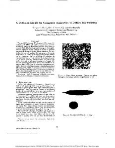
Fig. '.2. A time series showing the formAtion of an accretion disk as a result of a dynamic computer simulation . Because of the gravitational pull of the compact object, matter is pulled away (rom the red star forming a thin disk around the white dwarf.
Fig. 3.3. An evolved stationary accretion disk where the color coding represents the local temperature produced by viscous interaction of the particles.
90
the orientation of a body-fixed coordinate system (d. Fig. 2.5). The introduction of a body-fixed system is essential since in a space-fixed coordinate system the components of the tensor of inerlia of a rigid body are not constant, but depend on the position and orientation of the body in space in a complicated way. The definition of the body-fixed. system is arbitrary, however, a special choice, namely
the principal axes of inertia and the origin in the center of mass is very advantageous. In this system, the tensor of inertia takes a simple diagonal form
o
B
(3.16)
o
with
A =
f(~2 + (2)p({,~,()d{d~d(
B = fee
+ (2)p({, ~,()d{d~d(
C = fee
+ ~2)p({, ~,()d{d~d(
(3.17)
where A, B, C are the principle moments of inertia.
ri,_ , .•• Forces actins on a riaid body
In general, a number of forces act on the rigid body (d. Fig. 3.4) and the problem is the resulting motion in space. Using center-or-mass coordinates %c, !Ie, Zc and fixing the origin of the body-fixed e'1( -system at the centee of mass the equations of motion for the system decouple in an equation for the center of mass and one relative to it:
M14=P=LF;
t
=
~(ew)
-
(3.18a)
Dr: xF;) + L71
(3.18b)
91
Here M = f P d{d~d( denotes the total mass of the rigid body, F; the external forces, L the angular momentum and 'Ii the external torques relative to the center of mass. The motion of the center of mass can easily be calculated by integrating (3.180.). The integration of (3.lSb) needs a further processing since with respect to space-fixed axes the components of the tensor of inertia are, in general, time-dependent. Therefore, the time derivative in the space-fixed system must be expressed by the time derivative ~: in the rotating body·fixed system with the help of the general relation (3.12). Using (3.12) and 8 = const in the body-fixed frame, the Eulerian equations of motion of a rigid body follow immedi.tely from (3.18b) dL( (3.19.) dt
1t
dL, _ Bw, + w(wdA - C) = T, (3.19b) dt dL( (3.19c) dt Knowing the torques these equations can be integrated, yielding the components ""(,"".,,""( of the angular velocity projected on the body-fixed axes as functions of time. To arrive finally at the motion of the body-fixed system a further integration is necessary, namely the integration of the first-order differential equation system connecting the components w(,w" , w, with the Eulerian angles Q,fJ,"Y and their time derivatives, which can immediately be obtained from (2.13) 1 (W( cOS"Y + o. = - -:--:0 SIDfJ
w.,
w.,
. "Y )
Sin
sin "Y + cos "Y ..y = w( cot fJ COS..., - WI) cot fJ sin "Y + we
/J
=
W(
(3.20.) (3.20b) (3.20c)
Eqs. (3.1), (3.18a) and (3.20) represent the basic equations of motion for a point mass and for a rigid body. With given initial conditions for position and velocity and known external forces and torques the position of the center of mass and the orientation of the body-fixed axes can be calculated by means of a standard integration routine.
3.3 A simple example: the falling rod To warm up let us consider as a simple example a rod Creely falling down from a certain height, hitting the bottom and jumping off again. The rod possesses the mass M and the length 1. Its tensor of inertia B relative to the ccnter of mass and in the body-fixed sytem of the principle axes of inertia is of the fonn
B =
A (
0
o
0 0)
A 0 0 0
(3.21 )
with A= 11'lM12 . The rod is described by the three Cartesian coordinates Xc, Yc, Zc of its center of mass lying in the middle of the rod and by the two Eulerian angles a, P for the orient.tion. The third Eulerian angle "Y is without meaning since the principle moment of inertia around the axis is zero and , therefore, the rod is Dot able to rotate around this axis
92
w,
with the consequence that is zero. In free fall, the only external force is the gravity M 9 which acts on the center of mass. This is also the reason why the external torques vanish. Taking into account the above considerations the equations of motion (3.18a) and (3.19) simplify to (3.22a) Mzc == 0
Myc: =0 Mic - -Mg "'( = 0
w.,
= 0
(3.22b) (3.220) (3.22d) (3.22e)
•
which immediately can be solved analytically, yidding Yc: =
+ %eO v",ot + !leO
(3.23a) (3.23b)
Zc
1 , -'291 +vczot+zcO
(3.230)
Xc:
= vuot
(3.23d) (3.23+ 2.,;b·'·")1
= 0
Eqs. (3.30b,c) and (3.29c) determine the changes of the velocities during the impact. The values of the quantities immediately before the impact can be calculated from the solution (3.25) and depend uniquely on the initial conditions. Having the changes at hand the values of the positions at the impact and the values of the velocities immediately after the impact serve as initial conditions for the further motion until the next impact. In the second ease of a totally inelastic impact with z:fter = 0 and i: her = 0 the equations read L!z. _ zaher _ ibefore = _ibefore ====::-
•• • L1xe = x~her + ~ sin (~imp~t)!f'afttr _ x~efore _ ~ sin (tpiInP~t ),pbefore L1 zc
====::-
+ ~ sjn(??imp~t)L1~ = _:r~efore
iafter _ ibefort = _ ibtfore
••
-
. after
Zc
ollie -
-
•
(3.3Ia)
====::-
. after '2I cos (impact) tp tp -
·before
Zc
~ cos(lPimp~')L1~ = _i~efore
+ '2I cos(,,,impact),,;,befort T
T
(3.3Ib)
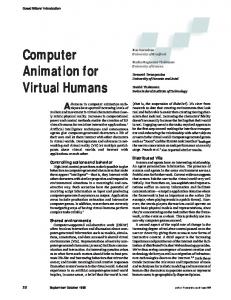
From (3.31a,b) and (3.29c) with the same procedure as above the motion can further be monitored. Of course, in this case the tot81 energy is not conserved. In Fig. 3.6 three stroboscopic time series of a falling rod are shown for different elastic behaviour of the ground. In the above considerations the impact is a point event in time. If one is interested in details during the impact the mechanical properties of the colliding parts must be taken into account. This requires the knowledge of the relation between the reaction
95
Fig.3.6. Three stroboscopic time series of a falling rod for an increasing (top to bottom) damping component in the ground reaetion force.
96
force and the local defonnalion and, if damping elements are present, the instantaneous deformation velocity. Inserting a realistic relation Fc(rddarm,'rdclorm) into the right hand sides of (3.28) and integrating numerically these equations yield all quantities as continuous functions of time even in the impact region, which is now exlented in a small time interval. As an example for a specific ground behaviour the following relations could
be used as components of the ground reaction force: Fer
= pFc,.
(3.32)
The vertical component of the ground reaction force depends on the defonnation and on the deformation velocity of the groundi Q, band d are material constants. The horizontal component of the ground reaction force is usually determined by friction and therefore proportional to Fe,.
4 Mechanics of multi-linked models for biomechanical simulations
For the modelling of human beings or animals with legs and arms multi-linked systems of extended bodies connected by joints are necessary. Developing a satisfactory model is by no means a trivial problem. The joints and their constraints must be correctly described as well as the mechanical properties of the body segments. Important is the action of external forces especially during short impacts and, finally, the time development of the internal torques in the joints, which are generated by the skeletal muscles and thus reflect the free will of the being to control its motion.
4.1 Description of a multi-linked system In principle, the mechanical problem of a multi-linked system has been solved for a long time. We will recapitulate some general facts.
4.1.1 Coordinates and degrees of freedom
Let us consider a system with n segments and n - 1 joints. At first , we will assume that the motion takes place in a plane. Then, each segment is defined by three coordinates, two cartesian coordinates for the position of the center of mass and one angle for the orientation {cf. Fig. 4.1a}. All together we have 3n coordinates and, therefore, we need 3n equations. In the plane case each joint yields two conditions, namely that the coordinates of the two end points of corresponding segments coincide. Taking into account these conditions we end up with 3n - 2(n - I} = n + 2 degrees of freedom. The number n + 2 is also the minimal number of coordinates needed for a unique description. These coordinates are free from
97
any restrictions. Additionally, we have three equations of motioo, two for the center of mass of the whole system and one for the motion relative to it. Thus , there remain n + 2 - 3 = n - 1 quantities undetennined, the torques in the n - 1 joints, the free will of the individual. An other way to consider the same subject is to regard each segment separately. In our plane case we Deed 3 coordinates (%ci, Zci,¥'i) for each segment and, with known forces and torques acting on the segment, the motion of its center of mass and relative to it can be obtained by numerically integrating the 3 equations of motion
Mjrci -
L LF L
Fijz
(4.1a)
ij ,
(4.1b)
1
j
(zjjFjjz -
ziJF:Jz) -
2: Tin
(4.1c)
j
1
(. )
(b)
z
(% " , ~, , )
ri,. ... I. (a) Coordinates of • plane multi· linked system. Each aqmf::nl ill defined by the Cartesian coordinates Z ci. ZCl of iLB c~nLer of mUll and an ans'e If'i determinins its orient.tion nlative to the hori~ontalline . (b) Forces and torques actins on the eqmenLs. Beside the edernal (orces like sravitation and sround reaction (orce additionally, (or the first joint, the internal (orces and torques are shown.
and Lj Ttj contain all forces and torques, external and internal, acting on the segment. The external forces such as gravitation, friction or contact forces must be given, the internal for ces are caused by the constraints of the joints. Due to actio = reactjo there are two unknown force components at a joint acting in opposite direction on the two segments connected by this joint. Since the condition of a joint yields two equations, the 2(n-l ) internal forces are uniquely determined by the 2(n - l) equations
EJ F'J
98
of the joint conditions. These forces are necessary to keep the segments together. The standard method to deal with such problems is the Langrangian Connalism. Solving the 30 + 2( n - 1) equations, the motion of the n connected segments and the internal joint forces are obtained simultaneously. The (n - 1) torques, of course, are free again and dctcnninc the active behaviour of the model . The same counting rhymes can be applied to a three dimensional model. To determine the degrees of freedom we nole that one segment needs six coordinates and the n - 1 joints yield 3(n - 1) conditions thus, the minimal number of free coordinates is given by 6n - 3(n -1) = 3n + 3. Taking into account the six equations of motion for the whole system, we end up with 3(0 - 1) fredy choosable internal torques. This number, however, is only valid for freely movable spherical ball joints.
4.1.2 Joints and constraints In the simulation of the motion of animals or human beings the modelling of joints is an essential part. Simple cases are hinge joints, which are movable around definite axes, or spherical ball joints, which are freely movable in three dimensions. For such joints the conditions for the connection of the two segments can easily be fonnulated as algebraic equations. An example for a ball joint is the human hip, one for a hinge joint is the human knee. The last is true only in a first approximation, a closer inspection exhibits a complex structure shown in Fig 4.2.
fi, .•. :z. Skeletal structure or the numan knee JOint with the different muacle and joint forces .
Far more complicated are joints without axes or points of rotation. Biological exam· pIes of such joints are the shoulders. Joints of this type can be modelled by introducing appropriate trunk· fixed and arm·fixcd surfaces, which roll and slide on each other. These surfaces must be individually detennined with the help of film analysis. A further important aspect in modelling joints is the range of mobility. Each joint possesses a definite range of angles for flection depending on the structure of the skeleton. During the course of animation sequences care must be taken that the joint angles do not exceed these biological limits. Of course, the most promising way is to imitate nature. When approaching the limiting angle in the joint an internal torque is built up which decelerates the motion and prevents an overshooting. This torque must depend on the difference of the actual joint angle and the limiting angle c,Plimit and on the angular velocity of the joint a.ngle. This velocity dependence is necessary to include a damping mechanism and thus to avoid an unnatural clastic reflection from the stop. A reasonable form of this torque is
99
- tpjoi.tl,~joi.t) = { ~a(l\Plim .. - \pjoiod)' + c]-'(1
T(ltpu~lt
+ d