Animating Suspended Particle Explosions. Bryan E. Feldman. James F. O'Brien. Okan Arikan. University of California, Berkeley. Abstract. This paper describes a ...
Computer Graphics Proceedings, Annual Conference Series, 2003
Animating Suspended Particle Explosions Bryan E. Feldman
James F. O’Brien
Okan Arikan
University of California, Berkeley
Abstract This paper describes a method for animating suspended particle explosions. Rather than modeling the numerically troublesome, and largely invisible blast wave, the method uses a relatively stable incompressible fluid model to account for the motion of air and hot gases. The fluid’s divergence field is adjusted directly to account for detonations and the generation and expansion of gaseous combustion products. Particles immersed in the fluid track the motion of particulate fuel and soot as they are advected by the fluid. Combustion is modeled using a simple but effective process governed by the particle and fluid systems. The method has enough flexibility to also approximate sprays of burning liquids. This paper includes several demonstrative examples showing air bursts, explosions near obstacles, confined explosions, and burning sprays. Because the method is based on components that allow large time integration steps, it only requires a few seconds of computation per frame for the examples shown. Keywords: Explosions, fire, combustion, computational fluid dynamics. natural phenomena, physically based animation. CR Categories: I.3.5 [Computer Graphics]: Computational Geometry and Object Modeling—Physically based modeling; I.3.7 [Computer Graphics]: Three-Dimensional Graphics and Realism—Animation; I.6.8 [Simulation and Modeling]: Types of Simulation—Animation
1
Introduction
Although explosions are thankfully rare occurrences for most people, they appear nearly ubiquitously in the synthetic environments we create. Movie and television plots often include them, and few video games omit them. Environments developed for training simulations frequently focus on violent or otherwise dangerous situations, so they also commonly include some form of explosive phenomena. This paper addresses the needs of these applications by presenting a fast, simple to implement, physically based method for animating realistic explosions such as the one shown in Figure 1. E-mail: {bfeldman|job|okan}@eecs.berkeley.edu
To appear in the proceedings of ACM SIGGRAPH 2003.
This work has been submitted or accepted for publication. Copyright may be transferred without further notice and the accepted version may then be posted by the publisher.
Figure 1: An explosion next to an immovable wall generated by detonating a small charge inside a mass of flammable particles.
The exact definition of an explosion varies depending on context, but generally an explosion comprises a sudden release of energy that creates an outward-propagating pressure front, or blast wave. Explosions may arise from mechanical (e.g. rupture of a compressed air cylinder), chemical, nuclear, or other events. The blast wave is an explosion’s primary effect, but it moves at supersonic speeds and its only visible manifestation is a subtle refraction of light. Except for extremely large, powerful explosions, the refraction effect is almost completely invisible. Secondary effects may include bright flashes of light, flame, dust, and flying debris. These secondary effects can be quite visibly noticeable. By design, the real explosions employed for visual effects typically minimize blast strength while maximizing the appearance of secondary effects. In particular, they feature large dramatic fireballs even when the situation purportedly shown would only produce minimal amounts of flame. One reason for this deviation from reality is that strong blast waves are hard to see yet exceedingly dangerous: both the
1
ACM SIGGRAPH 2003, San Diego, CA, July, 27–31, 2003
concussive force of a strong blast and high velocity shrapnel can be deadly even at a fair distance. In contrast, large fireballs look very impressive while being somewhat safer to work with. Both suspended particle explosions and liquid/vapor explosions can produce large fireballs. A suspended particle, or dust, explosion occurs when a highly flammable particulate such as gunpowder, coal, sawdust, or flour, is dispersed over a volume of air and then ignited. (We discuss an example coal-dust explosion in Section 5.) Possible dust dispersal mechanisms include vibrations or a smaller initial explosion. Liquid/vapor explosions occur similarly except rather than a flammable particulate it is a flammable liquid and its vapors that are dispersed and then ignited. One notorious example of a liquid/vapor dispersal scenario, known as a BLEVE (B oiling Liquid E xpanding V apor E xplosion), occurs when a closed container of flammable liquid is heated. The heat vaporizes liquid in the container, building pressure until the container ruptures and sprays a flammable mixture of liquid and vapor into the surrounding environment where it can then be ignited by whatever source had been heating the container. While accidental occurrences of both suspended particle and liquid/vapor explosions can be destructive and deadly, skilled pyrotechnicians can use them to sculpt the appearance of a desired effect. However, even in skilled hands, they are still expensive and potentially dangerous. This paper describes a simulation method designed to realistically model the behavior of suspended particle explosions. Although this method is intended primarily for situations involving particulates, we have found it to be flexible enough that it will work reasonably well for some scenarios involving burning liquid sprays. The method uses a relatively stable fluid dynamics simulation to compute the motion of air and hot gases around the explosion. Particles immersed in the fluid track the motion of particulate fuel and combustion products as they are advected by the fluid. The system models combustion using a simple but effective process governed by the particle and fluid systems. Unlike previous physically based approaches to animating explosions, this method does not attempt to model the numerically troublesome blast wave and other transient pressure phenomena generated by the explosion. Instead it uses a fast, incompressible fluid model and adjusts the divergence field to account for the generation of expanding gaseous combustion products. As a result, our Matlab implementation requires no more than a few seconds of computation per frame on a modest workstation to simulate the motion of even the largest of the examples presented here.
2
Background
Significant effort has been directed toward animating explosions and related phenomena such as fire. The earliest of this work appears in [Reeves, 1983] where particle systems were introduced as a means for modeling flames and other objects that lack hard boundaries. Particle systems remain one of the most commonly used methods for animating explosions, and numerous systems have been developed that make use of heuristic rules to move and shade particles so that they create the appearance of an explosion or fire. The primary strength and limitation of these systems is that they depend on a skilled user to select parameters that yield realistic results. To a large extent the method presented in this paper, as well as some of the prior physically based
2
approaches discussed in this section, are simply particle systems where the heuristic rules have been replaced with rules based more closely on the underlying physics. The physical basis facilitates achieving a realistic result for a wider range of conditions by adding rules that approximate those of the real world. Much of the previous work in graphics on physically based explosion modeling has focused on the blast wave and its effect on solid objects. In [Mazarak et al., 1999] and [Martins et al., 2002] the blast is approximated as an expanding spherical wave with a pressure profile determined by an analytical approximation to experimental data. When the expanding wave encounters voxelized objects in the environment, it applies radial forces to those objects. If the forces exceed a threshold then the inter-voxel connections will be broken. A similar approach appears in [Neff and Fiume, 1999] where they also account for the angle between the blast wave and object surface normals. A more accurate, but much more expensive, blast wave model appears in [Yngve et al., 2000] where the explosion is modeled using a compressible fluid simulation. Forces based on the pressure gradient are applied to objects in the environment causing them to move or fracture based on an algorithm described in [O’Brien and Hodgins, 1999] and [O’Brien et al., 2001]. Although this method models diffraction and reflection effects well, dealing with steep pressure and density gradients in the fluid makes the method computationally very expensive. In addition to modeling the blast wave, they also address modeling the secondary effects of flame and stirred dust. The primary differences between [Yngve et al., 2000] and the method presented here arise from focusing on modeling the flame associated with the explosion rather than the blast wave. Instead of using an illconditioned compressible fluid simulation, the method presented here uses an incompressible fluid simulation and generates the expansive flow caused by the explosion with constraints on the flow field’s divergence. The method presented here also includes a combustion model for generating more realistic fireballs. In addition to explosions, researchers in the graphics community have also investigated methods for modeling the motion of gases such as smoke or mist using three-dimensional fluid dynamics simulations. Some examples of this work include [Foster and Metaxas, 1997], [Stam, 1999], and [Fedkiw et al., 2001]. Our fluid model is based primarily on that of [Fedkiw et al., 2001]. Fluid models have been used to model fire as well. The method in [Stam and Fiume, 1995] uses a fluid model and noise to generate rising flames. In [Lamorlette and Foster, 2002] a variety of convincing flame effects, including large fireballs, are generated by simulating the motion of streamers in a turbulent flow and then applying fire textures to the streamers. A similar approach using particles is described in [Dalton et al., 2002]. A combustion model that tracks the motion of combustible gases on the fluid grid appears in [Melek and Keyser, 2002]. The method described in [Nguyen et al., 2002] generates realistic flames for situations where combustion occurs along a thin border between a flammable gas and an oxidizing environment. The combustion process generates heat and the fluid flow at the gas/air boundary is modified to account for expansion. While the method produces excellent results when rapid combustion occurs only along a thin front, it is not well suited to situations that spread the combustion region over a significant volume.
Computer Graphics Proceedings, Annual Conference Series, 2003
Other related work in graphics includes methods for modeling fire within buildings [Bukowski and S´equin, 1997], fire propagation over surfaces [Beaudoin et al., 2001; Lee et al., 2000; Chiba et al., 1994], and explosion-like effects [Bashforth and Yang, 2001]. A significant amount of effort has also been devoted to rendering realistic fire including [Rushmeier et al., 1995] and many of the papers referenced above. Outside of graphics, researchers have performed a substantial amount of work developing methods for simulating explosions and fire. A comprehensive review of that work falls outside the scope of this paper. The work that we believe to be most relevant to our approach is the Fire Dynamics Simulator (FDS) developed at the National Institute of Standards and Technology and described in detail in [McGrattan et al., 2002]. Our system has substantial similarity to FDS and our work was motivated in part by it. We considered building on the FDS code, but decided that the differences between the approach we wished to take and the one in FDS implied that developing our own system would be preferable. Some of the key choices we made different than in FDS include: computing advection terms using an unconditionally stable semi-Lagrangian scheme, using direct divergence constraints rather than large eddy approximation, enhancing the fluid motion using vorticity confinement, and tracking particulate reactants using a particle system.
3
Simulation Methods
Because the appearance of suspended particle explosions arises from the behaviors of the burning particulates, surrounding air, and combustion products, our method explicitly models each of these components and their interactions with each other. The user specifies the type of behavior to be simulated by setting initial conditions that will give rise to the explosion. Once configured, the system evolves according to rules that approximate the physical laws that govern motion, temperature, and combustion in the combined system. These rules have been designed so that the simulated behavior will qualitatively match observations taken from real explosions. For an overview concerning the properties of dust explosions see [Cashdollar, 2000].
3.1
Gas Model
We model the mixture of air and gaseous combustion products filling the environment where the explosion occurs using a slightly modified version of the fluid model described in [Fedkiw et al., 2001]. This model treats the gases as an incompressible, inviscid fluid that fills a rectilinear threedimensional grid. It determines the motion of the fluid to satisfy the requirements that momentum and mass be conserved. Momentum conservation is enforced by the Euler equations (Navier-Stokes with zero viscosity): u˙ = −(u · ∇)u − ∇p/ρ + f /ρ
(1)
where u is the fluid velocity, ρ density, p pressure, f any external forces acting on the fluid, and an overdot denotes differentiation with respect to time. We treat density as a constant for the fluid. The external forces include thermal buoyancy, vorticity confinement, and interactions with the particles. The first two are described respectively in [Foster and Metaxas, 1997] and [Fedkiw et al., 2001], and we will describe the last in Section 3.4. For an incompressible fluid, mass conservation requires that the velocity divergence be zero, however we will have
processes that add fluid to the environment or cause the fluid to expand. Instead of uniformly requiring zero divergence we require that for each fluid cell ∇·u=φ
(2)
where φ is zero everywhere except where some process is generating additional fluid or causing the existing fluid to expand by heating it. To enforce Equation (2) we simply solve a slightly modified version of Poisson’s equation ∇2 p =
ρ (∇ · u − φ) ∆t
(3)
to determine the fluid pressure within each cell. The same grid that holds the fluid’s velocity also holds the fluid’s temperature. The temperature evolves according to T˙ = −(u · ∇)T − cr
�
T − Ta Tmax − Ta
�4
+ ck ∇2 T +
1 ˙ H (4) ρcv
where T denotes the fluid temperature, Ta ambient temperature, Tmax the maximum temperature in the environment, and H heat energy transfered into the fluid. The first term models advection by the fluid. The second term loosely approximates radiative loss into the environment with cooling constant cr . The third is a diffusion term which would normally be insignificant, however we set an unrealistically large value for the thermal conductivity, ck , and use the term to approximate both radiative and diffusive transfer. The final term accounts for heat energy transfered into the fluid from an external source. We refer the reader to [Stam, 1999] for a description of how to solve these fluid equations efficiently. A detailed description of how to approximate the required derivatives on a regular staggered Cartesian grid appears in [McGrattan et al., 2002].
3.2
Particulate Model
We model the motion of both the particulate fuel and solid combustion products (soot) using a particle system. Particle descriptions consist of a position, velocity, mass, temperature, thermal mass, volume, and type identifier. Each particle’s behavior follows the simple rules ¨ = f /m x
˙ m Y˙ = H/c
(5)
where x denotes the location of a particle, f any external force on the particle (including gravity), Y the particle temperature, H heat energy transfered to the particle or generated by combustion, and cm the particle’s thermal mass. If the particles have very small mass/thermal mass we treat them as massless/thermally massless and dispense with the appropriate portion of Equation (5). Although we use a large number of particles (see Table 1), each simulated particle does not represent a single dust particle. Instead, each simulated particle represents a grouping of fuel or soot particles and the attributes of the simulated particle describe the group’s aggregate properties.
3.3
Detonation, Dispersal, and Ignition
Large fireballs may result from an initial high-velocity explosion that disperses particulate fuel over a volume while igniting it. As discussed previously, the primary result of
3
ACM SIGGRAPH 2003, San Diego, CA, July, 27–31, 2003
cles away from the detonation, but the motion may also be enhanced by applying an outward force directly to the particles. Although, we have found doing so largely unnecessary. In addition to fireballs, other effects may be achieved as well. For example, a jet may be modeled by forcing the fluid velocity at a location to a prescribed value, or a stream of fuel particles may be sprayed into the volume. By specifying conditions at various locations and times the user may design a desired event similar to how a pyrotechnician might design a real explosion by rigging physical devices, except that there is less risk of accidental injury. A final note about setting up the initial conditions for the simulation is that the starting fluid velocity should not be set to zero or any other spatially constant velocity. Doing so tends to produce undesirably symmetrical results. Instead the starting fluid velocities should be perturbed with small random seed values as described in [McGrattan et al., 2002].
3.4
Figure 2: These figures illustrate the result of injecting fluid at the center of a two-dimensional environment by setting a single cell’s divergence to a positive value. The left side shows the result when a relatively open set of obstacles surrounds the source. Above is a plot of the resulting pressure field, and below the resulting velocity field. The right side shows a more constraining configuration of obstacles.
this initial explosion is a rapid jump in pressure as the explosive detonates. The high pressure region creates a shock wave and propels the surrounding particulate fuel outward. The compressible fluid method used by [Yngve et al., 2000] to compute the blast’s behavior is expensive and incompatible with an incompressible fluid model. Instead we take an approach that models the outward flow from the initial detonation while explicitly ignoring wave behavior. In the region where the detonation occurs, the divergence constraint value, φ, rises rapidly until it reaches a peak value determined by the strength of the detonation. The value of φ in the region then decays back to zero, goes slightly negative, and finally stabilizes again at zero. This schedule approximates the pressure profile typical of a high-explosive detonation and it models the abrupt expansion and introduction of additional gases that occurs as the explosive vaporizes. The solver that enforces Equations (1) and (2) will generate a momentum-conserving flow field with zero divergence except where φ is non-zero. The result will be a discrete approximation to a continuous incompressible flow field that moves outward (or inward if φ < 0) from where expansion has occurred. The flow will correctly conform to obstacles and other divergence sources. The diagram in Figure 2 shows a pair of two-dimensional flow examples. In addition to affecting the flow field, a detonation may also heat the region where it occurred or impart a repulsive force directly on nearby particles. The heat added to the fluid accounts for heat generated by combustion of the explosive and isometric pressure increase. It changes the fluid temperature according to Equation (4). In the following section we discuss how the particle motion is affected by the fluid flow so that the outward flow will accelerate the parti-
4
Interaction and Combustion
The particle and fluid models interact with each other through the transfer of momentum and heat energy. Additionally, our combustion model involves interactions between the particles and fluid. As the particles move through the fluid they experience drag forces. The drag force on a particle is ˙ u − x|| ˙ f = αd r2 (¯ u − x)||¯
(6)
where αd is the particle’s drag coefficient, r its radius, and ¯ is the fluid’s interpolated velocity at the particle location. u The opposite force is applied to the fluid cell containing the particle. If the particle’s mass lies below a threshold, it is ¯ , leaving the fluid’s treated as massless and we set x˙ = u velocity unaffected. Thermal transfer between the particles and the fluid is handled in a similar fashion. The rate of heat transfer to a particle from the fluid around it is determined by H˙ = αh r2 (T¯ − Y )
(7)
where αh denotes the coefficient of thermal conductivity between the materials and T¯ the fluid’s interpolated temperature at the particle location. If the particle’s thermal mass falls below a threshold, then we set Y = T¯ and the fluid’s temperature remains unaffected. Some of the particles in the system represent particulate fuel. Once ignited, these particles generate the fiery mass of hot gases and soot that creates the appearance of a burning explosion. While the actual process of combustion is quite complex, we have found that good results can be obtained with a greatly simplified model. The three most significant simplifications we include are that combustion occurs irrespective of oxygen availability, that the combustion rate is invariant with temperature, and that the composition of combustion products does not depend on temperature either. We justify the first assumption because studies show that even at very high concentration, dusts suspended in air do not encounter a rich limit [Cashdollar, 2000]. In contrast, as the concentration of flammable gas in an air/fuel mixture increases it will eventually reach a point where the mixture is no longer explosive. For situations where flammable particulates have been suspended in air, oxygen will always be available. We make the other two assumptions for convenience. We expect that accounting for variations in burn rate or combustion products produced would not be overly
Computer Graphics Proceedings, Annual Conference Series, 2003
Figure 3: A series of images showing a single explosion over an infinite plane.
difficult, but we do not expect that it would significantly change the resulting appearance for the situations we are concerned with. A fuel particle will ignite when its temperature rises above its ignition point. Once ignited the particle will consume its own mass at a set rate, its burn rate, z. When the particle’s remaining mass reaches zero, it is deleted from the system. The burning particles generate heat, gaseous products, and solid products. Heat is generated at a rate H˙ = bh z
(8)
where bh is the amount of heat released per unit combusted mass of the fuel. The gaseous products are added to the fluid system by adding an increment to φ for the cell containing the burning particle ∆φ =
1 bg z V
Figure 4: A side-by-side comparison of our simulated results with a photograph of a staged coal-dust explosion in c the Bruceton Experimental Mine. (Photo 1986 Kenneth L. Cashdollar NIOSH-Pittsburgh Research Laboratory, used with permission.)
(9)
where V is the volume of the cell and bg the volume of gas released per unit combusted mass less the volume of gas consumed. The solid combustion products, commonly called soot, enter the system in the form of additional, inflammable, particles. As a fuel particle burns it generates soot mass at a rate (10) s = bs z where bs denotes the mass of soot produced per unit combusted mass of fuel. The created soot mass accumulates in a variable associated with the fuel particle. When a sufficient quantity has accumulated a soot particle will be generated. The initial position and velocity of the soot particle match those of the fuel particle with a small random perturbation. The true values of αd and αh depend on factors, such as the shape of the particles, that fall below the level of detail in this simulation. Similarly, the various burn constants may be adjusted to approximate known materials or they may be selected based on appearance. The values used here were selected to achieve desirable results. All of the examples we have created involved a single type of fuel that experiences a single combustion phase. Multiple fuels could be accommodated by including multiple types of fuel particles. Multiphase combustion could be accommodated by having the initial fuel particle emit other types of fuel particles that would experience the next combustion phase.
Figure 5: A top-down view of the simulated mine explosion shown in Figure 4. Scene props other than the mine itself have been removed for clarity. Scattering effects were not computed for rendering this view.
4
Rendering Methods
Although we focus primarily on generating appealing motion for the explosions, compelling exhibition of the motion requires that it be realistically rendered. Rendering realistic flames, however, presents a number of tough problems, and while other researchers (e.g. [Nguyen et al., 2002; Lamorlette and Foster, 2002; Rushmeier et al., 1995; Stam and Fiume, 1995]) have addressed some of these problems, clear differences between real and rendered flames persist. The rendering scheme we have implemented produces reasonable results that are sufficient for exhibiting the simulated motion.
5
ACM SIGGRAPH 2003, San Diego, CA, July, 27–31, 2003
Example
Figure
Grid Size
Cell Width
Particle Count
Burst near wall Single burst Coal mine Nozzle horizontal Nozzle down Multiple bursts
1 3 4&5 6 6 7
35×35×45 36×36×60 35×45×35 75×25×45 40×15×35 36×36×60
0.38 m 0.50 m 0.50 m 0.13 m 0.13 m 0.50 m
1,200,000 1,000,000 1,500,000 1,800,000 1,250,000 4,048,470
Simulation time per frame Mean Max CPU 4.5 sec 6.9 sec 5.6 sec 7.8 sec 7.4 sec 6.7 sec
5.7 sec 11.4 sec 8.2 sec 11.6 sec 10.7 sec 11.6 sec
3.06 MHz 3.06 GHz 3.06 GHz 3.06 GHz 3.06 GHz 3.06 GHz
Rendering time per frame Mean CPU P4 P4 P4 P4 P4 P4
.8 min .7 min — .6 min .8 min 1.8 min
2.53 GHz 2.53 GHz — 2.53 GHz 2.53 GHz 2.53 GHz
P4 P4 P4 P4 P4
Table 1: Simulation statistics. Particle counts indicate the maximum number of particles active at any given time. Simulation and rendering frames both correspond to 1/30th of a second intervals. (For example, the simulation of a burst near a wall only required approximately 2.3 minutes to compute one full second of motion.) Measured times do not include file operations. Omitted timings were unavailable at the time of publication.
cloud (including self shadowing) are computed using a deep shadow map [Lokovic and Veach, 2000]. Direct illumination of other objects by the particles and scattering by the particles is computed using the hierarchical method described in [Jensen and Buhler, 2002]. One area for further work is improving the rendering method. The images produced by the particle-based renderer have an objectionable grainy appearance in place of realistic fine-scale detail. Applying texturing techniques, such as those described by [Lamorlette and Foster, 2002], to the particles would likely improve the appearance of the explosions significantly.
5
Figure 6: Two flamethrower examples. In the top image, the nozzle is aimed horizontally. In the lower image the nozzle has been directed toward the ground.
The images of the flames arising from the explosion are generated by rendering the fuel and soot particles directly. Each particle receives illumination from the environment and, if sufficiently hot, glows with its own light. The light emitted from the hot particles is based on blackbody radiation [Meyer-Arendt, 1984], but we adjusted the mapping to match images of real explosions. Light in the environment includes direct illumination from traditional sources, light emitted by other particles, and light scattered by the cloud of particles. Direct illumination shadows cast by the
6
Results and Discussion
We have implemented the method described above and used our implementation to generate the examples shown in this paper. The accompanying video tape contains animations corresponding to these examples. Information about the size of each example along with the time required to simulate the motion and to render the images appears in Table 1. The parameters used to generate the examples are listed in Table 2. The simulation was implemented in Matlab and the renderer in C. Both run on Intel-based PCs. The sequence of images in Figure 3 shows an explosion occurring over an infinite plane. Initially, a concentrated mass of fuel particles sits centered in the image a short distance above the ground. When a charge within the mass detonates, it disperses and ignites the fuel particles. The heat and soot released by the burning fuel generates a rising fireball. Figure 1 shows a similar sequence where an immovable wall has been placed near the explosion. The wall alters both the initial dispersion and subsequent motion of the fireball. To help gauge the realism of our simulated results, Figure 4 shows a comparison with a photograph of an actual coal-dust explosion exiting the entrance of a mine [Cashdollar, 1986]. The explosion was produced by dispersing bituminous coal dust over the first 50 feet into the mine using detonating cord, and then ignited the dispersed dust using dynamite and black powder [Cashdollar, 2002]. We imitated the situation with our simulation by arranging barriers to form a tunnel that was filled with a nonuniform distribution of fuel particles. The particles were then ignited by a charge, creating the results shown. An additional top-down view of the simulated explosion appears in Figure 5. The pair of images in Figure 6 show an approximation of a flamethrower. We modeled this by injecting a stream of hot fuel particles into the fluid. While we feel the flamethowers look reasonable, simple particles do a poor job modeling the
Computer Graphics Proceedings, Annual Conference Series, 2003
Example
Figure
Thermal cr ck
Fluid ρ cv
Burst near wall Single burst Coal mine Nozzle horizontal Nozzle down Multiple bursts
1 3 4&5 6 6 7
1000 0 0 2000 2000 0
1 1 1 1 1 1
5 5 10 0 0 10
1 1 1 1 1 1
m
z
0.36 0.34 0.27 0.03 0.03 0.23
0.21 0.67 0.31 0.07 0.07 0.35
Fuel Particles cm bg bh 20.54 2.61 2300 20.54 1.69 745 13.69 3.25 975 2.64 0.43 3700 2.64 0.43 3700 5.67 1.67 450
αh 300000 300000 200000 18500 18500 90000
αd ∞ ∞ ∞ 750 750 ∞
m cm
Soot Particles bs
0.005 0.005 0.003 0.0002 0.0002 0.007
13.86 13.86 1.37 3.67 3.67 18.50
1 1 1 1 1 1
αh 6175 6175 2050 3700 3700 9250
αd ∞ ∞ ∞ 210 210 ∞
Table 2: Simulation parameters. The values shown were selected heuristically to obtain desirable results and they do not have any particular physical significance.
dynamics of a liquid stream. We expect that better results could be obtained by using a liquid simulation to model the stream. The example shown in Figure 7 demonstrates several explosions detonating near each other over a short time interval. The interactions between the blasts creates behavior that is distinctly different from that of the lone explosion shown in Figure 3. Similarly, interaction with the obstacles shown in Figures 8 and 9 also generates distinct behavior. The method we have presented provides an efficient tool for generating motion for suspended particle explosions. We have shown several examples exhibiting a range of behaviors. Because the method explicitly avoids modeling the numerically unstable blast wave, the examples only require a few seconds of computation per simulated frame. Areas for future work include burning liquid sprays, complex chemical reactions, and more realistic rendering methods.
Acknowledgments We thank the other members of the Berkeley Graphics Group for their helpful criticism and comments. This research was supported by NFS CCR-0204377, State of California MICRO 02-055, ONR MURI N00014-01-1-0890, and by generous support from Sony Computer Entertainment America, Intel Corporation, and Pixar Animation Studios. The images in this paper were rendered with Pixie, an open source renderer available from http://pixie.sourceforge.net.
References Bashforth, B., and Yang, Y.-H. 2001. Physics-based explosion modeling. Journal of Graphical Models 63, 1 (Jan.), 21–44. Beaudoin, P., Paquet, S., and Poulin, P. 2001. Realistic and controllable fire simulation. In Graphics Interface 2001, 159– 166. ´quin, C. H. 1997. Interactive simulation Bukowski, R., and Se of fire in virtual building environments. In Proceedings of ACM SIGGRAPH 97, 35–44. Cashdollar, K. L., 1986. Coal-dust explosion propogating outward from the mine portal. Symposium on Industrial Dust Explosions, June. Cashdollar, K. L. 2000. Overview of dust exportability characteristics. Journal of Loss Prevention 12 , 183–199. Cashdollar, K. L., 2002. Personal communication, Nov. Chiba, N., Ohkawa, S., Muraoka, K., and Miura, M. 1994. Two-dimensional visual simulation of flames, smoke and the spread of fire. The Journal of Visualization and Computer Animation 5, 1, 37–54. Dalton, P., Rosenblum, R., Huang, S.-C., Lee, L., and Driskill, H. 2002. Digital pyro for reign of fire. In Visual Proceedings of ACM SIGGRAPH 2002, 167. Technical Sketch.
Figure 7: Multiple detonations over an infinite plane. Time progresses from bottom to top.
Fedkiw, R., Stam, J., and Jensen, H. W. 2001. Visual simulation of smoke. In Proceedings of ACM SIGGRAPH 2001, 15–22.
7
ACM SIGGRAPH 2003, San Diego, CA, July, 27–31, 2003
Figure 8: An explosion under an immobile arch.
Figure 9: An explosion between a group of immobile pillars.
Foster, N., and Metaxas, D. 1997. Modeling the motion of a hot, turbulent gas. In Proceedings of ACM SIGGRAPH 97, 181–188. Jensen, H. W., and Buhler, J. 2002. A rapid hierarchical rendering technique for translucent materials. In Proceedings of ACM SIGGRAPH 2002, 576–581. Lamorlette, A., and Foster, N. 2002. Structural modeling of natural flames. In Proceedings of ACM SIGGRAPH 2002, 729–735. Lee, H., Kim, L., Meyer, M., and Desbrun, M. 2000. Meshes on fire. In EuroGraphics 2000 Workshop on Animation. Lokovic, T., and Veach, E. 2000. Deep shadow maps. In Proceedings of ACM SIGGRAPH 2000, 385–392. Martins, C., Buchanan, J., and Amanatides, J. 2002. Animating real-time explosions. The Journal of Visualization and Computer Animation 13, 2, 133–145. Mazarak, O., Martins, C., and Amanatides, J. 1999. Animating exploding objects. In Graphics Interface 99, 211–218. McGrattan, K. B., et al. 2002. Fire dynamics simulator (version 3) technical reference guide. Tech. Rep. NISTIR 6783, 2002 Ed., National Institute of Standards and Technology. Melek, Z., and Keyser, J. 2002. Interactive simulation of fire. In Pacific Graphics 2002, 431–432. Presented in poster session. Meyer-Arendt, J. R. 1984. Introduction to classical and modern optics. Prentice-Hall. Neff, M., and Fiume, E. L. 1999. A visual model for blast waves and fracture. In Graphics Interface 99, 193–202. Nguyen, D. Q., Fedkiw, R. P., and Jensen, H. W. 2002. Physically based modeling and animation of fire. In Proceedings of ACM SIGGRAPH 2002, 721–728. O’Brien, J. F., and Hodgins, J. K. 1999. Graphical modeling and animation of brittle fracture. In Proceedings of ACM SIGGRAPH 99, 137–146. O’Brien, J. F., Bargteil, A. W., and Hodgins, J. K. 2001. Graphical modeling and animation of ductile fracture. In Proceedings of ACM SIGGRAPH 2001, 291–294. Reeves, W. T. 1983. Particle systems — a technique for modeling a class of fuzzy objects. In Proceedings of ACM SIGGRAPH 83, 359–376.
8
Rushmeier, H., Hamins, A., and Choi, M. Y. 1995. Volume rendering of pool fire data. IEEE Computer Graphics & Applications 15, 4 (July), 62–67. Stam, J., and Fiume, E. L. 1995. Depicting fire and other gaseous phenomena using diffusion processes. In Proceedings of ACM SIGGRAPH 95, 129–136. Stam, J. 1999. Stable fluids. In Proceedings of ACM SIGGRAPH 99, 121–128. Yngve, G. D., O’Brien, J. F., and Hodgins, J. K. 2000. Animating explosions. In Proceedings of ACM SIGGRAPH 2000, 29–36.
Figure 10: Cutaway view of the explosion shown in Figure 7.