Anisotropic Gaussian Filtering using Fixed Point Arithmetic

ANISOTROPIC GAUSSIAN FILTERING USING FIXED POINT ARITHMETIC Christoph H. Lampert

Oliver Wirjadi

German Research Center for Artificial Intelligence (DFKI) 67663 Kaiserslautern, Germany [email protected]

Fraunhofer ITWM Models and Algorithms in Image Processing 67663 Kaiserslautern, Germany [email protected]

ABSTRACT Gaussian filtering in one, two or three dimensions is among the most commonly needed tasks in signal and image processing. Finite impulse response filters in the time domain with Gaussian masks are easy to implement in either floating or fixed point arithmetic, because Gaussian kernels are strictly positive and bounded. But these implementations are slow for large images or kernels. With the recursive IIRfilters and FFT-based methods, there are at least two alternative methods to perform Gaussian filtering in a faster way, but so far they are only applicable when floating-point hardware is available. In this paper, a fixed-point implementation of recursive Gaussian filtering is discussed and applied to isotropic and anisotropic image filtering by making use of a non-orthogonal separation scheme of the Gaussian filter. 1. INTRODUCTION Low-pass smoothing of noisy images is a common initial step in image processing systems. Due to its simplicity and optimality for additive white noise, Gaussian filters are most frequently used. Typically, isotropic ones are used, but adaptive anisotropic filters are also established tools for structure preserving smoothing. Implementation of Gaussian convolutions is straight-forward in the image and Fourier transform (FT) domains, where usually the latter is considered preferable for large images and large filter masks. However, in embedded hardware environments, such as smart cameras, computing the FT for the whole image is beyond the capabilities of the hard- and software. In these cases, implementations that work solely in the image domain are necessary. Three recent results in (possibly anisotropic) Gaussian filtering have opened new possibilities for fast implementations of such filters: Recursive 1D Gaussian filtering [1, 2] and the separation of 2D [3, 4] and nD [4] anisotropic Gaussian kernels. All of these were developed with CPUs in mind that are equipped with a floating-point unit (FPU). In this contribution, we propose a fast implementation of Gaussian filters with full covariance matrix in arbitrary dimension, which is adapted to integer-only CPUs. The fil-

ter loop relies on fixed-point calculations and can therefore be performed using only integer operations. On platforms where the compiler can emulate floating-point operations in software, we use this feature for the initialization of the filter coefficients, see Section 2.2 for details. It is done only once per image, and therefore does not cause a significant loss of performance. If a platform does not support this, the coefficients can be precomputed and tabularized. Although all PCs contain FPUs these days, many perspective targets for integer-based Gaussian filtering exist in the embedded market: FPGAs. Field-Programmable Gate Arrays (FPGAs) have attracted increasing attention for speeding up low level routines in the area of real-time image processing and computer vision [5]. Although FPGAs can be programmed to perform floating point operations, one usually tries to avoid this because it requires more logic gates than this is the case for integer operations. GPUs. Modern graphics cards contain very fast and highly parallel units for fixed-point arithmetic. They can use Gaussian filters e. g. to smoothly blend textures into each other. For surfaces that lie rotated in 3D-space, this requires anisotropic 2D-Gaussian filtering [6]. Mobile devices. An increasing number of embedded devices can perform image capture and image processing operations, e. g. mobile phones and PDAs with integrated digicam [7]. Gaussian denoising is of special importance there, because the camera quality is low. 2. INTEGER-ONLY GAUSSIAN FILTERING In this section, we describe how 1D-Gaussian filtering can be implemented in fixed-point arithmetic. In particular, we study recursive Gaussian filters which have O(1) runtime complexity per pixel. We show how the 1D-filter can be used for lowpass filtering of images in arbitrary dimension, isotropically as well as anisotropically. The result is an integer-only Gaussian filter for images that is a good enough approximation to replace its floating-point counterpart.

2.1. One-dimensional FIR Gaussian Filtering Filtering with a one-dimensional Gaussian means convolution with the Gaussian kernel g(x; σ 2 ) = √

1 2πσ 2

x2

e− 2σ2 ,

(1)

where σ 2 is the variance parameter. For a discrete signal f [x], the convolution can be implemented as a finite sum, F [x] =

K X k=−K

f [x − k]g[k]

for all x.

(2)

where g[k] is the discrete signal that is derived from sampling the Gaussian g at integer positions k ∈ Z and F is the filtered output. g[k] drops to 0 exponentially for k → ±∞, and it is therefore safe to truncate the originally infinite sum to a finite one. Typically, K is chosen as ⌈3σ⌉ or ⌈5σ⌉ where ⌈.⌉ means rounding to next larger integer. The result is called finite impulse response (FIR) Gaussian filter and from the formula it can be seen that it requires O(K) operations per pixel. The filter mask g[k] does not depend on x and therefore has to be calculated only once. A fixed point implementation of the convolution sum (2) is straight-forward at any accuracy. When all coefficients of g[k] are non-negative and smaller than 1, problems of overflow do not occur. This is the 1 case for σ > 2π ≈ 0.16, and smaller values for σ are unreasonable, because have a filter mask of only a single point. 2.2. One-dimensional IIR Gaussian Filtering The disadvantage of the FIR Gaussian filter is that its runtime depends linearly on σ. For large filter sizes, it therefore becomes slow. In 1995, Young and van Vliet came up with an alternative solution [1]. They proposed an infinite impulse response (IIR) filter that approximates the Gaussian to high order. Their filter uses a recursive scheme that calculates the filter output F for a whole line of samples in a two-step procedure: w[x] = f [x] +

3 X k=1

F [x] = Bw[x] +

bk w[x − k]

3 X

bk g[x + k]

for all x

for all x

(3)

(4)

k=1

w is a buffer of intermediate results, and b1 , b2 , b3 and B are filter coefficients that depend on σ, see [2]. By a careful choice of scale for the other parameters, B can be made 1. Because the number of operations necessary for each pixel is independent of σ, the filter has complexity O(1) per pixel. We implemented Eq. (3) and (4) in integer arithmetic, using 32 bit integer variables. 21 bits of those were reserved for the fractional part and 1 bit for the sign. Our choice was motivated by the fact that we work with [0:255] input data and

the fact that b1 , b2 and b3 stay in the range between −3 and 3. Thus, we require a sign bit, 8 + 2 = 10 bits for the integer part, and the rest of the 32 bits can be used to achieve as high accuracy as possible. Depending on the targeted hardware, other setups than a 1:10:21 split are of course possible. To implement the complete filter, additional constants are necessary, e. g. to control the boundary behavior. Some of those increase monotonically with σ and this limits the range of variance parameters for which our filter is applicable. With the chosen 1:10:21 split, σ 2 should not exceed a value of approximately 170 to avoid overflows in the computation. Larger values of σ can be reached by using more bits for the integer part or by exchanging the optimal boundary treatment by Triggs and Skida [8] for a simpler method. Further details about the implementation can be found in the source code of our reference implementation, which is available from the homepage of one of the authors1 . 2.3. Axis-Aligned Gaussian Filtering For higher-dimensional signals, e. g. 2D or 3D images, isotropic Gaussian filtering is defined analogously to the 1Dcase, by convolution with the Gaussian kernel of corresponding dimension. It is well known that its n-dimensional Gaussian kernel can be factorized into n one-dimensional Gaussians that are aligned to the coordinate axes: g(x; σ 2 ) = √

1 2πσ 2

e−

||x||2 2σ 2

=

n Y

g(xi ; σ 2 ).

(5)

i=1

Here, ||x|| is the length in Rn of the coordinate vector x = (x1 , . . . , xn ). Because of Equation (5), the Gaussian convolution integral is separable, and the n-dimensional Gaussian filter can be calculated as a sequence of n one-dimensional Gaussian filter steps, one along each of the coordinate axes. FIR or IIR filters can be used for this, as have been studied in the previous section. Equation (5) can be generalized to arbitrary axis-aligned filtering by allowing different variance parameters σ12 , ..., σn2 in each direction xi : g(x; Σ) =

1

1

t

p e− 2 x (2π)n/2 |Σ|

Σ−1 x

=

n Y

g(xi ; σi2 ), (6)

i=1

where Σ denotes the diagonal matrix of variance parameters. The slightly more general factorization in (6) is useful for anisotropic image filtering as well, when the constraint of Σ being diagonal is dropped. For this, it has to be combined with a shear operation as explained in the following section. 2.4. Anisotropic Gaussian Filtering To construct general anisotropic Gaussian filters, we lift the restriction of the previous section and consider arbitrary positive definite covariance matrices Σ. The form of the Gaussian 1 http://www.iupr.org/∼chl/

function remains the same as in the left-hand side of (6). Such Gaussians in n dimensions have n(n+1) degrees of freedom. 2 n of those are the variance parameters σ12 , . . . , σn2 and the remaining parameters can be interpreted as rotation angles for the filtering directions. How such an anisotropic Gaussian filter can be computed with O(1) complexity per pixel was first explained in [3] for R2 . Our explanation follows [4], where for the general case of Rn it is shown that anisotropic Gaussian filtering of an image is equivalent to the following procedure: • Calculate the Triangular Factorization of Cholesky Type of the covariance matrix Σ. That is, a decomposition Σ = V DV t , where D is a diagonal matrix and V is upper-triangular with unit diagonal.

If the shear parameters are integer valued, the shear is just a memory copy operation. However, in our setup the shear coefficients, which are derived from the entries of V and V −1 , are not integer-valued, and therefore the expression on the right hand side points to a location between pixel positions. There are now two choices: either one rounds the position to the nearest integer, then the shear is reduced to a pure copy operation again. Or, one applies interpolation of the image information, linearly in the 2D case and bilinearly in 3D. This requires calculation of the fractional parts of the pixel position and the weighted sum of 2 or 4 neighboring pixels. This can be done in fixed point arithmetic using an arbitrary number of precision bits. 3. RESULTS

• Transform the image linearly using the matrix V −1 . Because of the special form that V has, this operation is a shear. • Apply axis-aligned Gaussian filtering with covariance matrix D. • Shear the image back, i. e. transform it linearly using the matrix V . 2.4.1. Triangular Factorization The triangular factorization matrices V and D can be calculated with elementary operations +, −, ×, : from the entries si,j of Σ. E. g. for 2-dimensional images, we have v1,1 = 1,

v1,2 =

d21 = s1,1 −

s1,2 , s2,2

s21,2 ,r s2,2

v2,1 = 0,

v2,2 = 1

d22 = s2,2

(7) (8)

where (vi,j )i,j=1,2 are the entries of the matrix V and d21 , d22 the diagonal elements of D. A derivation can be found in [3]. For 3D and the general case, see [4]. These operations can easily be executed in fixed point arithmetic, with the additional advantage that the d2i values are always positive and never larger than the entries of Σ. v1,2 can be positive or negative, but unless the Gaussian becomes very strongly elongated, it is of modulus less than 1. 2.4.2. Forward and Backward Shear

(9)

I is the input image here, and O is the resulting output. x and y are the pixel coordinates and α is the shear parameter. For 3-dimensional images, the formula is similar: O[x, y, z] = I[x + αy + βz, y + γz, z]

3.1. Signal Filtering Accuracy The floating-point versions of the recursive Gaussian filter are known to be good approximations of the true Gaussian. A major concern when using only integer operations for such a recursive filter is the question whether the multiple executions of the filter loop Equations (3) and (4) will accumulate rounding errors when applied to long filter lines. For that reason, we performed experiments as in Figure 1, where we applied the fixed point IIR filter implementation to a synthetic signal counting 2000 samples. The enlarged detail of the beginning and end of the signal show that there is no accumulation of errors. The differences between fixed and floating point implementations in Fig. 1(d) are magnitudes below the actual signal content, showing that the 1+10+21 split that we chose guarantees sufficient accuracy. 3.2. Image Filtering Accuracy

A shear transformation of a 2-dimensional image is given by O[x, y] = I[x − αy, y].

In the previous sections, we have explained how arbitrary Gaussian filters can be implemented without using floatingpoint calculations in the filter loop. In this section, we show that the corresponding fixed-point versions are good approximations to their floating-point counterparts and to the true Gaussian. For this, we tested our implementation using a reconfigurable network camera as an embedded Linux system. The camera is powered by an ETRAX 100LX 32-bit RISC CPU at 100 Mhz. Floating point functionality is only available as emulation at severely reduced execution speed.

(10)

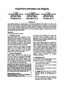
For 2D filtering we relied on two applications of the 1D recursive filter, as was outlined in Section 2.3 and 2.4. Figure 2 shows impulse responses of our fixed point implementation for the isotropic and anisotropic cases. The comparison to the corresponding true Gaussian functions shows a close approximation. We can therefore conclude that the previous results on the accuracy of the IIR filter for signal and image processing remain valid for a fixed point implementation.

20 10 0

10

256

256

(a) A signal of 2000 samples with additive, independent noise.

−10

2000

impulse response Gaussian −10

0

10

20

−20

−10

0

10

20

128

128

−20

−20

1500

−10

1000

−20

500

0

0

128

20

256

256 128 0

0

0

0

float int 0

500

1000

1500

2000

Fig. 2. 2D impulse response of our fixed-point IIR implementation vs. the true Gaussian function: isotropic (σ12 = σ22 = 150) and anisotropic (σ12 = 100, σ22 = 150, φ = 45◦ ).

167

172

168

176

169

180

(b) The filtered signals using floating and fixed point implementations.

2

4

6

8

10

1992

1994

1996

1998

2000

2e−04 0e+00 −2e−04

2e−04 −2e−04

0e+00

(c) Details of the figure above, at the beginning and end of the signal.

0

500

1000

1500

2000

(d) Difference of float and fixed point filter results.

Fig. 1. Fixed vs. floating point IIR filtering (σ = 8.0) applied to a signal. No accumulation of rounding errors towards the end of a long filter line can be observed. 4. CONCLUSION We have presented a method for Gaussian image filtering that uses only a constant number of integer operations per pixel. As a main contribution we introduced a fixed point implementation of a one-dimensional recursive Gaussian filter and its integration into an anisotropic Gaussian filter setup. By dispensing with floating-point calculations in the main filtering loop, the method is suitable e. g. for embedded platforms where floating-point operations are computationally expensive, because they have to be emulated in software. With a lookup table of precomputed parameter values, the method can also work without any floating-point operations, which is suitable e. g. for GPUs and FPGAs. Our analysis of the filter’s accuracy showed that an implementation using 32 bit integers is sufficient to give results that are virtually identical to a floating-point implementation. It is also possible to reduce the necessary resources by using

fewer fractional bits, but this comes at a sacrifice of accuracy. 5. REFERENCES [1] Ian T. Young and Lucas J. van Vliet, “Recursive Implementation of the Gaussian Filter,” Signal Processing, vol. 44, pp. 139–151, 1995. [2] Ian T. Young, Lucas J. van Vliet, and Michael van Ginkel, “Recursive Gabor Filtering,” IEEE Transactions on Signal Processing, vol. 50, no. 11, pp. 2798–2805, 2002. [3] Jan-Mark Geusebroek, Arnold W. M. Smeulders, and Joost van de Weijer, “Fast Anisotropic Gauss Filtering,” IEEE Transaction on Image Processing, vol. 23, no. 8, pp. 938–943, 2003. [4] Christoph H. Lampert and Oliver Wirjadi, “An Optimal Non-Orthogonal Separation of the Anisotropic Gaussian Convolution Filter,” Technical Report 82, Fraunhofer ITWM, Kaiserslautern, Germany, 2005, submitted to IEEE Transactions on Image Processing. [5] Bruce A. Draper, J. Ross Beveridge, A. P. Wim B¨ohm, Charles Ross, and Monica Chawathe, “Accelerated Image Processing on FPGAs,” IEEE Transactions on Image Processing, vol. 12, no. 12, pp. 1543–1551, 2003. [6] Mario Botsch and Leif Kobbelt, “High-Quality PointBased Rendering on Modern GPUs,” in 11th Pacific Conference on Computer Graphics and Applications (PG’03), 2003, p. 335. [7] Maurizio Pilu and Stephen Pollard, “A Light-Weight Text Image Processing Method for Handheld Embedded Cameras,” in Proceedings of the British Machine Vision Conference, September 2002. [8] Bill Triggs and Michael Sdika, “Boundary Conditions for Young - van Vliet Recursive Filtering,” To appear in IEEE Transactions on Signal Processing, 2006.