Annealing Based Dynamic Learning in Second-Order Neural Net works Srdjan Milenkovidl , Zoran Obradovid21*and Vanto Litovskil 'Department of Electronic Engineering, University of Nii, Beogradska 14, 18000 NiS, Yugoslavia. School of Electrical Engineering and Computer Science, Washington State University, Pullman, WA 99164-2752, USA. e-mail:
[email protected] ABSTRACT An algorithm that simultaneously determines an appropriate number of neurons and their interaction parameters in a single hidden layer feed-forward neural network (NN) classification model is proposed. First, a large pool of candidate hidden units with second-order inputs interaction is constructed. Next, the hidden layer is designed by selecting appropriate units from the pool. This is achieved through global hidden layer optimization by a simulated annealing technique that adds and deletes hidden units as needed. Experimental results using the proposed model show improved generalization and reduced complexity as compared t o previous constructive learning algorithms based on greedy design techniques.
1. Introduction Determining an appropriate NN topology is a challenging problem that usually requires a n expensive trialand-error process. Rather than learning on a pre-specified network structure, the algorithm proposed in this paper learns network topology as well. The advantage of such a learning approach is that the network size is automatically fitted to the input patterns without over-specializing, which often results in better generalization. In this paper we consider NN design for binary classification problems, where every training pattern pi E P belongs to one of two classes C1 or Cz. The problem is mapped onto a feed-forward NN with n inputs, a single layer of hidden units and a single output level unit, whose two states represent classes C1 and C z . The aim of this study is t o determine automatically the appropriate number of neurons for the hidden layer, as well as the neurons weight parameters, through supervised learning using patterns from P . This research was inspired by a greedy constructive neural network algorithm called the Hyperplane Determination from Examples (HDE) which suggests a discrete approach to neural network optimization suitable for parallel and distributed implementation [l]and a promising technique for integration of prior symbolic knowledge and learning from examples [2]. The objective of this study is t o overcome the HDE local minima problem by allowing hidden units with higher representational power and by performing
optimization with better global optimization properties (as compared to the previous greedy approach) through a simulated annealing technique for NN construction. The model is described in more detail in Section 2, the algorithm in Sections 3 and 4, and the experimental results in Section 5. Research sponsored in part by the NSF research grant NSF-IFU-9308523.
0-7803-3210-5/96 $4.0001996 IEEE
458
2. The Second-Order Neural Network Model Let U = (ul, u2, ...,un) be a neuron's input, and let f : Rn + R be its input interaction function. On input the output of a bipolar neuron with threshold t is computed as g(f(u) - t ) , where g : R -+ {-1,1} is defined as g(z) = 1 iff z 2 0. Here, we consider neurons with input interactions of the form:
U,
n
n
n
i=l
i=l
n
n
i=l
i=l
n-1
n
i = l j=i+l
where wi(l),wj2) are weight parameters associated t o the i-th input value U;, while wi(:) is a weight associated to the product of the i-th and j - t h input values U; and uj. Neurons with interaction functions described by (11, (2) and (3) will be referred t o as hyperplane (HP), flat ellipsoid (FE) and slant ellipsoid (SE) neurons respectively. Feed-forward neural networks constructed with HP neurons alone are called first-order NN, while NNs having neurons of all three types are called second-order NNs.
3. Candidate Pool Construction In binary classification, the hyper-surface separating two disjoint subregions C1 and C2, is called a problem decision boundary. In a feed-forward neural network each hidden neuron partitions the problem domain into two disjoint subregions separated by a neuron decision boundary that is defined by f ( U ) - t = 0, where f(u) is the neuron interaction function. A neural network combines decision boundaries defined by its hidden neurons into a more complex hyper-surface called a network: decision boundary. The objective of neural network design is to construct a network decision boundary that approximates the problem decision boundary reasonably well. A boundary dipole is represented by a pair of neighboring training patterns ( p , , p b ) , such that p , E C1, and pb E C2. For a two dimensional problem, this is illustrated in Fig. l(a). To obtain a correct classification of the training data, the network decision boundary has t o cross all boundary dipoles defined by the training set data. The points where the NN decision boundary crosses the segments defined by each dipole are called boundary CTOSS points. As the boundary cross points positions are not known a priori, in our algorithm they are initially positioned at the midpoint of the dipoles and are later moved t o more optimal positions as explained in the following section. Similar t o [l],in the proposed algorithm the candidate pool construction starts with a search procedure on the training data with the objective of finding a sufficient number of boundary dipoles. Next, to generate candidate neurons of HP, F E and SE type, each boundary dipole found in the search procedure is grouped with its n - 1, 2n - 1 or 2n n(n - 1)/2 - 1 nearest boundary dipoles respectively, where the distance is measured between the corresponding boundary cross points. Boundary dipoles are grouped in sets of size n, 2n and 2n n(n - 1)/2 as that many weight parameters determine a n HP, FE and SE neuron respectively. Grouping neighboring boundary dipoles is motivated by the assumption that it is more probable for neighboring boundary points than for distant boundary points to define a useful neuron decision boundary. Finally, each group of boundary cross points is used to compute a neuron's initial parameters by solving a linear system of n, 2n, or 2n n(n - 1)/2 equations of the form (l),(2) or (3) determined by these points.
+
+
+
4. Hidden Layer Optimization The pool of HP, F E and SE neurons, constructed as explained in Section 3, contains a large number of candidates for the hidden layer. The goal of this stage of the algorithm is t o select a small set of neurons
459
current neuron decision boundary new neuron decision boundary
Fig. 1: (a) Network Boundary Parameters, and (b) a Neuron Boundary Update
from this pool that gives a good generalization when used as a NN hidden layer. In the previous HDE algorithm [l]the NN’s hidden layer is constructed using a greedy approach that might end up in a local minimum in some cases. To avoid this problem, we use a simulated annealing approach to optimize both the hidden layer structure and the interconnection weights simultaneously. Simulated annealing is an iterative optimization procedure known to have better global optimization properties as compared to the greedy approach. It uses the analogy between the cooling process of a physical system and an optimization problem [3]. The algorithm starts by choosing a n initial solution and an initial temperature. Next, the cost of the current (initial) solution is calculated and two iterative loops (inner and outer) are started. The inner loop first generates a new solution through modification of the current one and computes its cost. A new solution is unconditionally accepted if it costs less than the current one, and is accepted with some temperature dependent probability otherwise. The inner loop iterates until the system reaches a steady state for a given temperature. The outer loop controls the whole process by decreasing the temperature parameter until convergence by using a specific annealing schedule. In our algorithm, the initial NN hidden layer is constructed using a t least one HP, one F E and one SE neuron randomly selected from the candidate pool constructed in Section 3. To generate a new hidden layer from the current hidden layer, one of the following update moves is randomly performed: Neuron activation: randomly select one inactive unit from the candidate pool and activate it (i.e. insert it in the hidden layer). Neuron deactivation: randomly deactivate one active unit (i.e. remove a hidden neuron and return it to the candidate pool). Neuron swap: randomly deactivate one active unit and activate one inactive unit. Boundary cross point change: for a randomly selected active unit, move one of its defining boundary cross points along the corresponding boundary dipole segment and recalculate its weights. A new boundary cross point position is chosen randomly from the region defined by a rank limiter as illustrated in Fig. l ( b ) for a cross point change of a H P neuron in a two dimensional space. A rank limiter is centered about the current position of the cross point and, initially, its length is large enough t o cover the whole dipole region. As the annealing temperature decreases the cross point position is closer t o the optimum, and so the rank limiter range is reduced as a function of temperature without the risk of ending up in a local minimum. As a consequence, the annealing search is faster due t o a smaller number of possible solutions. The cost of a newly generated hidden layer is a function of the classification error E (total number of misclassification) and the number of HP, FE and SE hidden neurons denoted as Hhp, H f e , and H , ,
460
I
Hidden Units Training Accuracy Test Accuracy Method Avg. Min Max Avg. Best Worst Avg. Best Worst HDE 6.4 6 8 73.60 78.11 67.89 66.73 68.98 63.67 1-1-1 11.4 8 15 94.32 96.45 I 91.12 73.93 77.08 71.76 3-3.5-4 II 2.2 I 1 I 3 I 86.75 I 93.49 I 62.13 I 73.20 II 81.82 II 63.89 1-00-00 10.4 7 13 94.32 96.45 92.32 75.92 84.72 69.44
I
I
I
I
I
Table: 1: The
I
I I
I
I I
I
I
I
I
I
I
I
MONK-2 Problem: Complexity and Generalization
respectively. This cost is evaluated as
+ max(0, H - Hma,}, (4) where the second term H = chpHhp + c f e H f e + cdeHdereflects the hardware complexity, and the third Cost = E + H
Cf
term represents an overfit penalty. User specified constants H, and cf control the number of neurons in the hidden layer, while chp, cf,, and cde represent the relative importance parameters of the corresponding neuron types. For binary classification problems, a single HP neuron in the output layer is sufficient. After the NN hidden layer is optimized, determining the output neuron parameters is a simple task that is performed using the pocket algorithm [4]. This algorithm yields optimal parameters with arbitrary high probability if it is run long enough.
5. Experimental Results In order to test the proposed learning algorithm, experiments were performed on several benchmark problems. In all experiments the overfit penalty constants in the cost function (4) are fixed to cf = 1 and H,,, = 20.
5.1. The MONK-2 Problem MONK’S problems consist of three standard benchmarks in which robots are classified in one of two groups based on a six multiple-valued attributes description [5]. The simplest problem, MONK-1, is designed to test system’s ability to discover a rule combining attributes in a simple disjunctive normal form. More difficult MONK-3 problem is an extension of MONK-1 designed to test learning of a disjunctive normal form in the presence of noise. Finally, MONK-2 is designed to test system’s ability to learn from data generated by a rule which combines attributes in a way which is quite complicated to describe in a disjunctive or conjunctive normal form. In MONK-1, MONK-2 and MONK-3 problems, the learning task is to generalize by learning from a subset of 124, 169 and 122 robots respectively. The HDE constructive algorithm is reported [I] to perform well on MONK-1 and MONK-3 tests (comparable to algorithms designed through extensive trial and error procedure) with 96.66% and 94.00% average generalization accuracy over five runs. However, the HDE is also reported to have local minimum problems when applied to a more complex MONK-2 test, resulting in 66.73% average generalization accuracy over five runs. The objective of our first set of experiments was to test if a more global optimization approach proposed in this paper can improve the MONK-2 generalization by avoiding a local minimum problem experienced using a greedy HDE network construction. The experiments measure the average, the maximum and the minimum number of hidden units in generated NN’s, as well as the average, the best and the worst accuracy on the training and on the test set over five runs with different initialization parameters. The experimental results on MONK-2 test obtained using the HDE constructive learning algorithm are shown in the first row of Table 1. The second row, labeled as the 1-1-1 method, summarizes results obtained using the proposed annealing based constructive approach with hardware penalty parameters for the HP, FE and SE hidden neurons
46 1
0.
00
Fig. 2: Effectiveness of the Second-Order (a) vs. First-Order (b) Model
(used in the annealing cost function 4) having an identical value chp = cfe = c,, = 1. The obtained accuracy on the training patterns is much better than using the HDE method (average accuracy of 94.32% vs. 78.11%) indicating that the proposed simulated annealing based dynamic construction method is indeed avoiding the local minimum problem experienced using the HDE greedy construction. The accuracy on unseen test patterns using the 1-1-1method is also better than the generalization result obtained using the HDE construction (average accuracy of 73.93% vs. 66.73%). On MONK-2 problem, training set accuracy of the 1-1-1method is much better than its generalization on test patterns. This indicates an overfit problem due to overemphasized classification error penalty component in the annealing cost function. Consequently, in the next set of experiments, the penalty for hidden units is increased to reduce the influence of the classification error. In addition, in these experiments the cost function coefficients of chp = 3, cf, = 3.5 and c,, = 4 reflect larger cost for neurons of more complex decision boundary. The result of these experiments, labeled as the 3-3.5-4 method and summarized in the third row of Table 1, is significant hardware complexity reduction (2.2 versus 11.4 hidden units on average) without any damage t o the generalization scores of the 1-1-1method. The final set of experiments on the MONK-2 problem was performed to determine if the proposed annealing based construction can be used without second order FE and SE hidden neurons. The experiments on MONK-2 problem using a first order simulated annealing based dynamic system, resulted in better generalization and networks of somewhat smaller complexity as compared t o the 1-1-1system. The results summary for these experiments are labeled as l-00-00 and shown in the fourth row of Table 1. 5.2. Four Embedded Circles Problem
This problem consists of 120 two-dimensional training patterns lying on four circles with a joint center. The patterns on the smallest and the largest circle belong to class C1 while the remaining patterns belong to class Cz. The task is to construct a classifier able to distinguish between the two classes. To compare the effectiveness of the proposed second order versus the first order simulated annealing construction, this problem is solved using both the first and the second-order annealing based dynamic learning NN's. The cost function parameters chp = 1/3 and chp = cfe = c,, = 1 are used in the first-order and the second-order model experiments, respectively. In the second-order NN experiment, hardware cost parameters are larger due to a smaller expected number of units in the hidden layer.
462
The decision boundary obtained using the second-order model with HP, FE and SE neurons is shown in Fig. 2a, while a boundary restricted to HP neurons alone is shown in Fig. 2b. The second-order solution results in a smaller number of neurons (5 vs. 19) and better accuracy (100% vs. 98.33%) which justifies the introduction of F E and SE neurons. For comparison, an HDE constructed NN for this problem had 10 hidden units and the best accuracy averaged over five experiments of only 83.33%, further demonstrating that the proposed annealing based dynamic approach is more likely to avoid the local minimum problem. In our experiments, the smallest back-propagation based NN for this problem that obtained 100% accuracy had 11 hidden units. The back-propagation solution also deteriorates drastically (to below 86.67% accuracy) if the number of hidden units is smaller than 11, showing that the trial and error network construction approach can easily miss the desired minimal topology.
6. Conclusion A NN efficiency and generalization ability depends strongly on the selected neuron model, network architecture and learning algorithm. The proposed global optimization algorithm automatically and simultaneously modifies both the network structure and the neuron interaction parameters in a second-order feed-forward NN. Results on several benchmark problems indicate that both the simulated annealing based network optimization and the second order neurons can be useful in improving a neural network generalization and reducing its complexity.
Acknowledgements The authors are grateful to Justin Fletcher for providing an implementation of his HDE constructive learning algorithm for comparison.
References [l] J. Fletcher and Z. Obradovic. A discrete approach to constructive neural network learning, Neural, Parallel and Scientific Computations, vol. 3, no. 3, pp. 307-320,1995. [2] J. Fletcher and Z. Obradovic. Combining prior symbolic knowledge and constructive neural network learning, Connection Science, vol. 5, no. 3-4,pp. 365-375,1993. [3] S. Kirkpatrick et al. Optimization by simulated annealing, Science, vol. 220, no. 4598, pp. 671-680, 1983. [4]S. I. Gallant. Perceptron-based learning algorithms, IEEE Trans. on Neural Networks, vol. 1, no. 2, pp. 179-191,1990. [5] S.B. Thrun et al. The MONK’S problems: A performance comparison of different learning algorithms, Technical report, Department of Computer Science, Carnegie Mellon University, 1991.
463