Anomaly Clustering in Hyperspectral Images Timothy J. Dostera , David S. Rossa , David W. Messingerb , William F. Basenera a Rochester
Institute of Technology School of Mathematical Sciences, Rochester, NY; Institute of Technology Center for Imaging Science, Rochester, NY
b Rochester
ABSTRACT The topological anomaly detection algorithm (TAD) differs from other anomaly detection algorithms in that it uses a topological/graph-theoretic model for the image background instead of modeling the image with a Gaussian normal distribution. In the construction of the model, TAD produces a hard threshold separating anomalous pixels from background in the image. We build on this feature of TAD by extending the algorithm so that it gives a measure of the number of anomalous objects, rather than the number of anomalous pixels, in a hyperspectral image. This is done by identifying, and integrating, clusters of anomalous pixels via a graph theoretical method combining spatial and spectral information. The method is applied to a cluttered HyMap image and combines small groups of pixels containing like materials, such as those corresponding to rooftops and cars, into individual clusters. This improves visualization and interpretation of objects. Keywords: graph theory, TAD, clustering
1. INTRODUCTION A hyperspectral image, in contrast to a multispectral image, has in general hundreds of spectral bands instead of one to ten spectral bands. For example, in the Cooke City image that is used throughout the paper, there are 126 channels1 . A normal digital image can be viewed as having three spectral bands (blue, red, and green), but in hyperspectral images a more extensive and continuous part of the light spectrum is represented. Hyperspectral images include spectral bands representing the visible, near-infrared, and shortwave infrared and thus are favored over multispectral images for some applications such as forestry and crop analysis as well as military exercises. Clustering is the grouping of like pixels from an image together based on their characteristics, typically their spectral response. The level of cluster differentiation is a choice of the user. For example the user can choose to cluster all trees into one group or have a cluster of elms, pines, and oak trees. An anomalous, for this research, is one that has some degree of dissimilarity from the rest of the pixels in the image. For most algorithms this measure is based solely on the spectral information. In more classic applications of anomaly detection Gaussian statistics are used - this however, from a theoretical aspect, would require that the image’s pixels follow a normal distribution. For a naturally-occurring image, i.e. one that is not artificially created, this will not be the case. The most popular of these detection algorithms, which we will briefly describe in the next section is the RX algorithm2 . The Topological Anomaly Detection Algorithm3 , TAD, addresses this shortcoming in the RX Algorithm. The output of TAD however only declares anomalous pixels, it does not give a true count of the number of anomalous objects in an image. For example it may be advantageous to have all the anomalous pixels making up a camouflage net be grouped together and called one whole anomaly. The extension to the TAD algorithm discussed in this paper does just that. It improves the visualization of anomalies by differentiating between point anomalies and those that belong to a larger group. Further author information: (Send correspondence to W.F.B) W.F.B: E-mail:
[email protected]
Algorithms and Technologies for Multispectral, Hyperspectral, and Ultraspectral Imagery XV, edited by Sylvia S. Shen, Paul E. Lewis, Proc. of SPIE Vol. 7334, 73341P · © 2009 SPIE CCC code: 0277-786X/09/$18 · doi: 10.1117/12.818407 Proc. of SPIE Vol. 7334 73341P-1
2. RX ALGORITHM The RX algorithm developed by Reed and Yu2 in simplest terms finds the mean of the data and flags any pixels that have values far away from the mean as anomalies. Each pixel is surrounded by a sliding box that is centered on that pixel. The covariance of the data inside the box is then calculated. The rank of the pixel is the number of standard deviations that the pixel and the background model differ by; alternatively, the background model can be based on the entire image. The algorithm works well as long the image can be assumed to have normally distributed data. The problem, however, arises that hyperspectral images, even after dimensionality reduction, cannot be guaranteed to follow a gaussian distribution.
3. TOPOLOGICAL ANOMALY DETECTION ALGORITHM The Topological Anomaly Detection Algorithm3 differs from the RX algorithm in that no assumption on the normality of the data is made. It has been shown to perform better with much higher consistency then that of statistically-based anomaly detection algorithms such as the RX algorithm. The algorithm has also been shown to perform particularly well as a method for characterising the background of an image. TAD works simply by constructing a graph of the data then characterising components of the graph, based on their sizes, as backgrounds or anomalies. A brief outline of the algorithm is below. Step 1: Let X be a finite collection of pixels that are k dimensional. Construct the graph, Gr , where r ∈ R+ is some threshold. A graph is a finite nonempty collection of objects called vertices together with a set of pairs of distinct vertices called edges4 . For Gr let X be the vertex set and define the edge set, E, such that for u,v ∈ X, uv ∈ E if and only if the spectral distance from pixel u to v is less than r. Step 2: Let H be a component of Gr . A component is defined as a connected subgraph such that the vertex set and the edge set of the subgraph are proper subsets of the vertex set and edge set of graph respectively and there is path that connects all the vertices of the component4 . Each component of G should represent a different type of material that is found in the image. If H contains at least p%, where p ∈ (0, 100) and denoted the background percentage, of the total pixels then it is background; otherwise it is an anomaly. Typically we let p = 2. Step 3: Let ω be an anomalous pixel. We now calculate the rank of ω by summing the distances to its third, fourth and fifth closest neighbors. This rank will be our measure of the anomalousness for ω. The TAD algorithm can be run on a moderen laptop, with a resonable data set (∼ 106 pixels), in approximatly two minutes.
4. ANOMALY CLUSTERING ALGORITHM This improvement to the TAD algorithm seeks to differentiate between point anomalies and anomalies consisting of several pixels. Challenges arise because of the uncertainty of the environment in which the image was taken for example anomalies that we would like to group can have drastically different shapes (blobs, lines, polygons) and can be split between encompassing a whole pixel and part of a pixel. The anomaly clustering algorithm extension works by post-processing the results of the TAD algorithm as follows: Step 1: Let X be the set of pixels obtained from the TAD algorithm. For each pixel value x ∈ X we know that x ∈ [0, 1]. This is the measure of how anomalous that pixel is with the larger the value of x being the more anomalous x is. Let N be a subset of X containing only pixels that are greater than some δ ∈ (0, 1). This allows us to pick out only the most anomalous pixels and thus those that will be most interesting in the final analysis. For our
Proc. of SPIE Vol. 7334 73341P-2
work we used δ = 0.5. Let k be the size of N . Step 2: Let M be an k × k matrix, where the pixels contained in N make up both the columns and rows, we will call it our detection matrix. Let i,j ∈ N . We define M (i, j) = 1 if i and j are connected. Here, we define connected as pixels that are spatially adjacent and within γ spectral radians (in spectral angle). Other metrics for connectedness can also be developed, but we have not used any here. We define spatially adjacent strictly to mean pixels that share a common edge in the image. Otherwise M (i, j) = 0. Note that M (i, i) = 1. Step 3: We now calculate Fk = M + M 2 + M 3 + . . . + M k . The (i, j) entry of M t represents the number of paths from point i to j in t moves4 . For our purposes we care only if there is a path between points i and j (not the number of paths) so we reduce all non-zero entries to 1. We iterate until we have reached solution equilibrium, that is until the k th and k th + 1 iteration are equal. Step 4: In the ith row of F , any non zero entries will belong to the same anomaly cluster as the ith pixel of X since they can be reached in a finite number of moves from pixel i. This means that they are anomalous compared with the background but are connected, and estimated to be the same material based on the spectral angle measure. We color these groups accordingly. The Anomaly Clustering Algorithm can be run on a moderen laptop computer, for a resonably-sized set of pixels (∼ 106 pixels), in approximatly five minutes.
4.1 Example The following simple example demonstrates how the anomaly clustering algorithm works. For this example let the following grid represent pixels we have determined to be anomalies and the values displayed be calculated spectral measures. Let γ = 0.01.
0.10
0.11
0.48
0.90
0.15
0.12
0.46
0.47
0.14
0.13
0.95
0.48
0.15
0.49
0.48
0.47
We now construct the detection matrix, designating the pixels in the grid from left to right, top to bottom:
Proc. of SPIE Vol. 7334 73341P-3
⎛ ⎜ ⎜ ⎜ ⎜ ⎜ ⎜ ⎜ ⎜ ⎜ ⎜ ⎜ ⎜ ⎜ M = F1 = ⎜ ⎜ ⎜ ⎜ ⎜ ⎜ ⎜ ⎜ ⎜ ⎜ ⎜ ⎜ ⎜ ⎝
1 1 0 0 0 0 0 0 0 0 0 0 0 0 0 0
1 1 0 0 0 1 0 0 0 0 0 0 0 0 0 0
0 0 1 0 0 0 0 0 0 0 0 0 0 0 0 0
0 0 0 1 0 0 0 0 0 0 0 0 0 0 0 0
0 0 0 0 1 0 0 0 1 0 0 0 0 0 0 0
0 1 0 0 0 1 0 0 0 1 0 0 0 0 0 0
0 0 0 0 0 0 1 1 0 0 0 0 0 0 0 0
0 0 0 0 0 0 1 1 0 0 0 1 0 0 0 0
0 0 0 0 1 0 0 0 1 1 0 0 1 0 0 0
0 0 0 0 0 1 0 0 1 1 0 0 0 0 0 0
0 0 0 0 0 0 0 0 0 0 1 0 0 0 0 0
0 0 0 0 0 0 0 1 0 0 0 1 0 0 0 1
0 0 0 0 0 0 0 0 1 0 0 0 1 0 0 0
0 0 0 0 0 0 0 0 0 0 0 0 0 1 1 0
0 0 0 0 0 0 0 0 0 0 0 0 0 1 1 1
0 0 0 0 0 0 0 0 0 0 0 1 0 0 1 1
⎞ ⎟ ⎟ ⎟ ⎟ ⎟ ⎟ ⎟ ⎟ ⎟ ⎟ ⎟ ⎟ ⎟ ⎟ ⎟ ⎟ ⎟ ⎟ ⎟ ⎟ ⎟ ⎟ ⎟ ⎟ ⎟ ⎟ ⎠
which gives us the first iteration anomaly clustering, since none of the rows of M are identical we cannot group any of the pixels together in this iteration as we see in the next figure.
0.10
0.11
0.48
0.90
0.15
0.12
0.46
0.47
0.14
0.13
0.95
0.48
0.15
0.49
0.48
0.47
Since the second iteration of the algorithm, M + M 2 , does not produce a different anomaly clustering, we will skip to the third iteration and calculate: ⎛ ⎜ ⎜ ⎜ ⎜ ⎜ ⎜ ⎜ ⎜ ⎜ ⎜ ⎜ ⎜ ⎜ 3 M =⎜ ⎜ ⎜ ⎜ ⎜ ⎜ ⎜ ⎜ ⎜ ⎜ ⎜ ⎜ ⎜ ⎝
4 5 0 0 0 3 0 0 0 1 0 0 0 0 0 0
5 7 0 0 0 6 0 0 1 3 0 0 0 0 0 0
0 0 1 0 0 0 0 0 0 0 0 0 0 0 0 0
0 0 0 1 0 0 0 0 0 0 0 0 0 0 0 0
0 0 0 0 4 1 0 0 6 3 0 0 3 0 0 0
3 6 0 0 1 7 0 0 3 6 0 0 1 0 0 0
0 0 0 0 0 0 4 5 0 0 0 3 0 0 0 1
0 0 0 0 0 0 5 7 0 0 0 6 0 0 1 3
0 1 0 0 6 3 0 0 10 7 0 0 6 0 0 0
⎞ 1 0 0 0 0 0 0 3 0 0 0 0 0 0 ⎟ ⎟ 0 0 0 0 0 0 0 ⎟ ⎟ 0 0 0 0 0 0 0 ⎟ ⎟ 3 0 0 3 0 0 0 ⎟ ⎟ 6 0 0 1 0 0 0 ⎟ ⎟ 0 0 3 0 0 0 1 ⎟ ⎟ 0 0 6 0 0 1 3 ⎟ ⎟ 7 0 0 6 0 0 0 ⎟ ⎟ 7 0 0 3 0 0 0 ⎟ ⎟ 0 1 0 0 0 0 0 ⎟ ⎟ 0 0 7 0 1 3 6 ⎟ ⎟ 3 0 0 4 0 0 0 ⎟ ⎟ 0 0 1 0 4 5 3 ⎟ ⎟ 0 0 3 0 5 7 6 ⎠ 0 0 6 0 3 6 7
Proc. of SPIE Vol. 7334 73341P-4
and then compute M + M 2 + M 3 , reducing iteration. ⎛ 1 1 0 0 ⎜ 1 1 0 0 ⎜ ⎜ 0 0 1 0 ⎜ ⎜ 0 0 0 1 ⎜ ⎜ 0 0 0 0 ⎜ ⎜ 1 1 0 0 ⎜ ⎜ 0 0 0 0 ⎜ ⎜ 0 0 0 0 F3 = ⎜ ⎜ 0 1 0 0 ⎜ ⎜ 1 1 0 0 ⎜ ⎜ 0 0 0 0 ⎜ ⎜ 0 0 0 0 ⎜ ⎜ 0 0 0 0 ⎜ ⎜ 0 0 0 0 ⎜ ⎝ 0 0 0 0 0 0 0 0
all nonzero entries to 1 we get the detection matrix for the third 0 0 0 0 1 1 0 0 1 1 0 0 1 0 0 0
1 1 0 0 1 1 0 0 1 1 0 0 1 0 0 0
0 0 0 0 0 0 1 1 0 0 0 1 0 0 0 1
0 0 0 0 0 0 1 1 0 0 0 1 0 0 1 1
0 1 0 0 1 1 0 0 1 1 0 0 1 0 0 0
1 1 0 0 1 1 0 0 1 1 0 0 1 0 0 0
0 0 0 0 0 0 0 0 0 0 1 0 0 0 0 0
0 0 0 0 0 0 1 1 0 0 0 1 0 1 1 1
0 0 0 0 1 1 0 0 1 1 0 0 1 0 0 0
0 0 0 0 0 0 0 0 0 0 0 1 0 1 1 1
0 0 0 0 0 0 0 1 0 0 0 1 0 1 1 1
0 0 0 0 0 0 1 1 0 0 0 1 0 1 1 1
⎞ ⎟ ⎟ ⎟ ⎟ ⎟ ⎟ ⎟ ⎟ ⎟ ⎟ ⎟ ⎟ ⎟ ⎟ ⎟ ⎟ ⎟ ⎟ ⎟ ⎟ ⎟ ⎟ ⎟ ⎟ ⎟ ⎟ ⎠
Using the third iteration detection matrix we find third iteration anomaly clustering map:
Similarly we can calculate: ⎛ ⎜ ⎜ ⎜ ⎜ ⎜ ⎜ ⎜ ⎜ ⎜ ⎜ ⎜ ⎜ ⎜ 4 M =⎜ ⎜ ⎜ ⎜ ⎜ ⎜ ⎜ ⎜ ⎜ ⎜ ⎜ ⎜ ⎜ ⎝
16 20 0 0 0 13 20 29 0 0 1 25 0 0 4 0 0 0 0 0 0 4 0 0 0 1 0 0 17 5 13 25 0 0 5 30 0 0 0 0 0 0 0 0 0 0 0 0 1 5 0 0 25 15 5 14 0 0 14 25 0 0 0 0 0 0 0 0 0 0 0 0 0 1 0 0 13 5 0 0 0 0 0 0 0 0 0 0 0 0 0 0 0 0 0 0
0 0 0 0 0 0 0 0 0 0 0 0 16 20 20 29 0 0 0 0 0 0 13 25 0 0 0 1 1 5 5 14
1 5 0 0 5 14 0 0 0 0 0 0 0 0 0 0 25 14 0 0 15 25 0 0 0 0 0 13 0 0 0 25 44 30 0 0 30 31 0 0 0 0 4 0 0 0 0 30 25 14 0 0 0 0 0 5 0 0 0 14 0 0 0 25
Proc. of SPIE Vol. 7334 73341P-5
0 0 0 0 1 0 0 0 0 0 0 0 0 0 0 0 13 0 0 0 5 0 0 0 0 0 1 5 0 1 5 14 25 0 0 0 14 0 0 0 0 0 0 0 0 5 14 25 17 0 0 0 0 16 20 13 0 20 29 25 0 13 25 30
⎞ ⎟ ⎟ ⎟ ⎟ ⎟ ⎟ ⎟ ⎟ ⎟ ⎟ ⎟ ⎟ ⎟ ⎟ ⎟ ⎟ ⎟ ⎟ ⎟ ⎟ ⎟ ⎟ ⎟ ⎟ ⎟ ⎟ ⎠
and then compute M + M 2 + M 3 + M 4 , reducing all nonzero terms to 1, we get the detection matrix for the fourth iteration: ⎛ ⎜ ⎜ ⎜ ⎜ ⎜ ⎜ ⎜ ⎜ ⎜ ⎜ ⎜ ⎜ ⎜ F4 = ⎜ ⎜ ⎜ ⎜ ⎜ ⎜ ⎜ ⎜ ⎜ ⎜ ⎜ ⎜ ⎜ ⎝
1 1 0 0 0 1 0 0 1 1 0 0 0 0 0 0
1 1 0 0 1 1 0 0 1 1 0 0 1 0 0 0
0 0 1 0 0 0 0 0 0 0 0 0 0 0 0 0
0 0 0 1 0 0 0 0 0 0 0 0 0 0 0 0
0 1 0 0 1 1 0 0 1 1 0 0 1 0 0 0
1 1 0 0 1 1 0 0 1 1 0 0 1 0 0 0
0 0 0 0 0 0 1 1 0 0 0 1 0 0 1 1
0 0 0 0 0 0 1 1 0 0 0 1 0 1 1 1
1 1 0 0 1 1 0 0 1 1 0 0 1 0 0 0
1 1 0 0 1 1 0 0 1 1 0 0 1 0 0 0
0 0 0 0 0 0 0 0 0 0 1 0 0 0 0 0
0 0 0 0 0 0 1 1 0 0 0 1 0 1 1 1
0 1 0 0 1 1 0 0 1 1 0 0 1 0 0 0
0 0 0 0 0 0 0 1 0 0 0 1 0 1 1 1
0 0 0 0 0 0 1 1 0 0 0 1 0 1 1 1
0 0 0 0 0 0 1 1 0 0 0 1 0 1 1 1
⎞ ⎟ ⎟ ⎟ ⎟ ⎟ ⎟ ⎟ ⎟ ⎟ ⎟ ⎟ ⎟ ⎟ ⎟ ⎟ ⎟ ⎟ ⎟ ⎟ ⎟ ⎟ ⎟ ⎟ ⎟ ⎟ ⎟ ⎠
Using the detection matrix from the fourth iteration we find fourth iteration anomaly clustering map:
Proc. of SPIE Vol. 7334 73341P-6
Finally we calculate M + M 2 + M 3 + M 4 + . . . + M 16 , reducing all nonzero terms to 1, we get the final detection matrix: ⎛
F16
⎜ ⎜ ⎜ ⎜ ⎜ ⎜ ⎜ ⎜ ⎜ ⎜ ⎜ ⎜ ⎜ =⎜ ⎜ ⎜ ⎜ ⎜ ⎜ ⎜ ⎜ ⎜ ⎜ ⎜ ⎜ ⎜ ⎝
1 1 0 0 1 1 0 0 1 1 0 0 1 0 0 0
1 1 0 0 1 1 0 0 1 1 0 0 1 0 0 0
0 0 1 0 0 0 0 0 0 0 0 0 0 0 0 0
0 0 0 1 0 0 0 0 0 0 0 0 0 0 0 0
1 1 0 0 1 1 0 0 1 1 0 0 1 0 0 0
1 1 0 0 1 1 0 0 1 1 0 0 1 0 0 0
0 0 0 0 0 0 1 1 0 0 0 1 0 1 1 1
0 0 0 0 0 0 1 1 0 0 0 1 0 1 1 1
1 1 0 0 1 1 0 0 1 1 0 0 1 0 0 0
1 1 0 0 1 1 0 0 1 1 0 0 1 0 0 0
0 0 0 0 0 0 0 0 0 0 1 0 0 0 0 0
0 0 0 0 0 0 1 1 0 0 0 1 0 1 1 1
1 1 0 0 1 1 0 0 1 1 0 0 1 0 0 0
0 0 0 0 0 0 1 1 0 0 0 1 0 1 1 1
0 0 0 0 0 0 1 1 0 0 0 1 0 1 1 1
0 0 0 0 0 0 1 1 0 0 0 1 0 1 1 1
⎞ ⎟ ⎟ ⎟ ⎟ ⎟ ⎟ ⎟ ⎟ ⎟ ⎟ ⎟ ⎟ ⎟ ⎟ ⎟ ⎟ ⎟ ⎟ ⎟ ⎟ ⎟ ⎟ ⎟ ⎟ ⎟ ⎟ ⎠
Using the final detection matrix, F, we get the final anomaly clustering map
We are able to see now that that the pixel grid has two large anomalies, one with six pixels and the other with seven, and it has three single-pixel anomalies as well.
Proc. of SPIE Vol. 7334 73341P-7
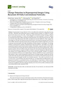
5. RESULTS The image used for analysis is of Cooke City, Montana, and was collected in July of 2006 using a HyMap sensor operated by HyVista. It contains 126 spectral bands, is 800x280 pixels, and has approximately 3 meter resolution5 . In the image there is a small town with several buildings, roads, cleared fields, and vehicles; the rest of the image is forest. The following figures were created using IDL and ENVI with the ENVI color mapping function.
,
.'
Figure 1. From top to bottom the original image, the TAD rendering of the image, and the anomaly clustering algorithm of the original image
6. CONCLUSIONS The anomaly clustering algorithm proved that it can create clusters of anomalous objects that are spatially contiguous and have similar spectral signatures. It made the differentiation between point anomalies and those that are much larger clearer. The algorithm offered evidence that an algorithm that relies on combining spectral and spatial information to make clustering determination is advantageous to just spatial or spectral alone. This can facilitate the analysis of the image by giving a truer sense of the relation of anomalies that are close together. For example it allows an analyst to see that a concentration of anomalies is actually 2 large objects that are composed of different materials and several other small singular pixel anomalies as we noted in the example above. Also if the analyst is looking for larger anomalies, ones that encompass more space than one pixel, such as buildings, the algorithm can reduce the number of anomalies that must be examined.
Proc. of SPIE Vol. 7334 73341P-8
7. FURTHER WORK The anomaly clustering algorithm can be refined with other metrics for measuring spectral connectedness. We have also discussed lowering the /delta value in the algorithm to allow more anomalies to be clustered together and give more detail in the processed image. Finally we would like to also make both these constants (δ and γ) defined by attributes of the image not by the user. The work discussed in this paper uses graph theory to group anomalies. We are have also done work on a statistics based anomaly classification algorithm on the premises of principal component analysis. We will be continuing this research next with the application of a manifold based anomaly classification algorithm, local linear embedding, to hopefully better differentiate between anomalies.
ACKNOWLEDGMENTS The authors would like to thank Dr. John Kerekes for supplying the data used in this paper, which can be found at http://dirsapps.cis.rit.edu/blindtest.
REFERENCES 1. J. Schott, Remote Sensing the Image Chain Approach, Oxford University Press, New York, 1997. 2. D. Manolakis, D. Marden, and G. Shaw, “Hyperspectral Image Processing for Automatic Target Detection Applications”, in Lincoln Laboratory Journal, Volume 14, Number 1, 2003. 3. B. Basener, E. Ientilucci, and D. Messinger, “Anomaly Detection Using Topology”, in Algorithms and Technologies for Multispectral, Hyperspectral, and Ultraspectral Imagery XIII, S. Shen and P. Lewis ed., Proceedings of the SPIE, Volume 6565, pp. 65650J, 2007. 4. G. Chartrand and L. Lesniak, Graphs and Digraphs, Chapman and Hall, New York, 2005 (fourth edition). 5. D. Snyder, J. Kerekes, I. Fairweather, R. Crabtree, J. Shive and S. Hager, Development of a Web-Based Application to Evaluate Target Finding Algorithms, Retrieved March 10, 2009, from Rochester Institute of Technology, Center for Imaging Science Web sit, http://www.cis.rit.edu/people/faculty/kerekes/pdfs/IGARSS 2008 Snyder.pdf.
Proc. of SPIE Vol. 7334 73341P-9