to use graphical models such as Bayesian Networks. (BN) [3] [4]. BNs allow the learning of a model that captures the relationship between the channels of hy-.
Probabilistic Classification of Hyperspectral Images by Learning Nonlinear Dimensionality Reduction Mapping
∗
X. Rosalind Wang, Suresh Kumar, Fabio Ramos, Tobias Kaupp, Ben Upcroft, Hugh Durrant-Whyte ARC Centre of Excellence for Autonomous Systems (CAS) Australian Centre for Field Robotics (JO4) The University of Sydney, NSW 2006, Australia { r.wang, s.kumar, f.ramos, t.kaupp, upcroft, hugh } @cas.edu.au Abstract - In this paper, we combined the application of a non-linear dimensionality reduction technique, Isomap, with Expectation Maximisation in graphical probabilistic models for learning and classification of hyperspectral image. Hyperspectral image spectroscopy gives much greater information content per pixel on the image than a normal colour image. This should greatly help with the autonomous identification of natural and man-made objects in unfamiliar terrains for robotic vehicles. However, the large information content of such data makes interpretation of hyperspectral images time-consuming and user-intensive. Isomap is used to find the underlying manifold of the training data. This low dimensional representation of the hyperspectral data facilitates the learning of a mixture of linear models representation similar to a mixture of factor analysers, the joint probability distributions of the model can be calculated offline. The learnt model is then applied to the hyperspectral image at run-time and data classification can be performed. We also show the comparison with results from standard techniques.
Keywords: Probabilistic Learning, Hyperspectral Imaging, Nonlinear manifold.
1
Introduction
Hyperspectral image spectroscopy is an emerging technique that obtains data over a large number of wavelengths per image pixel over an area. Spectral analysis is the extraction of quantitative or qualitative information from reflectance spectra based on the wavelengthdependent reflectance properties of materials [1]. Hyperspectral sensors are characterised by the very high spectral resolution that usually results in hundreds of observed wavelength channels per pixel of the image. These channels permit very high discrimination capabilities in the spectral domain including material quantification and target detection. The application of infrared reflectance spectroscopy with Short-Wave Infrared (SWIR, light from 1300 to 2500 nanometre ∗ This work is supported by the ARC Centre of Excellence programme, funded by the Australian Research Council (ARC) and the New South Wales State Government.
in wavelength) also allows recognition of subtle mineralogic and compositional variation [2]. Currently, the process of hyperspectral analysis is user intensive, requiring a large amount of data analysis, and expert input. The hyperspectral data is often represented as a “cube” of information where the layers of the cube are the images at the spectral bands. Systems are available for the simultaneous viewing of this information in the spatial and spectral domains [1]. The user is able to select points on the image and the program displays the spectrum at the specified location and the closest spectral match to it. The user then applies his/her own knowledge and other methods to interpret the data. While most methods of spectral analysis require a large amount of knowledge and understanding in spectroscopy and field sites, there are some that do not and can be applied in a relatively straightforward manner. The most widely used of these methods is Principal Component Analysis (PCA) [1]. The method, however is linear and scene specific, and thus hard to port to different regions and environmental conditions. Another method of analysing hyperspectral data is to use graphical models such as Bayesian Networks (BN) [3] [4]. BNs allow the learning of a model that captures the relationship between the channels of hyperspectral data [5] [6]. The classification of new data can then be inferred from the model. It is, however, computationally intensive: a Tree Augmented Naive Bayes Network, for example, has a time complexity of O(n2 · N ), where n is the number of vertices and N is the number of nodes in the network [4]. In this paper, we present a non-linear manifold mapping algorithm, Isomap, as described by Tenenbaum et al. [7] in combination with statistical learning as a method for analysing hyperspectral data. The Isomap algorithm is able to reduce the high dimensional data into a low dimensional manifold efficiently. This mapping of data from high to low dimension can then be learnt through a graphical model, along with the labels of the data. by applying the Expectation Maximisation algorithm [8], thus allowing us to classify the data. This paper is organised as follows. In Section 2, we present the data collected for the study. In Section 3, we first describe the Isomap algorithm in detail. The
4000 grass road trees water
3500
Reflectance
3000 2500 2000 1500 1000 500 0 0.6
0.8
1
1.2
1.4
1.6
1.8
2
2.2
2.4
Wavelength (µ m)
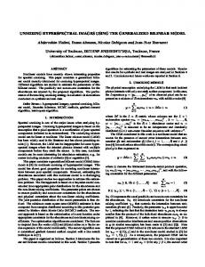
Figure 2: Spectra of the training data.
Figure 1: Hyperspectral image data of the Marulan test area, north is up, image is approx. 2 km across, the image is 3500 × 512 pixels in size. probabilistic methods used for learning the relationship between the manifold learnt from Isomap and the hyperspectral data as well as how the labels are fit within the model is then discussed. Finally in Section 4, we present the experimental results, compare it with results from some standard methods and discuss the shortcomings of the algorithm, and any improvements that can be achieved in the future.
2
Data collection
A hyperspectral visible near-infrared and short wave infrared (0.4 - 2.5 µm) dataset was collected in Australia near Marulan, New South Wales, roughly 200km south west from Sydney. The dataset was collected using the 125 band HyMap instrument [9] at an altitude of approximately 1.5km covering approximately 150km2 with an average resolution of 3.3m per pixel. The dataset was collected on 24th February, 2005 between 1200-1300 hours for maximum sunlight exposure. The test area allows access to a wide range of rural conditions such as grass land, river, trees, farm animals, man-made objects like buildings, as well as wildlife areas. This gives us a good place to test for learning representations of natural objects in a rural environment. The dataset was collected over the area because it is used extensively as a testing ground for both the air and ground robotic vehicles by our group. It is hoped that having air surveyed hyperspectral image data would give ground vehicles more information for navigation before deployment in an unknown natural
environment where there is no geometrical shapes for easy identification. Training data is necessary for an autonomous system to learn from the typical data it might encounter during operation. For our purposes, we require a set of training data that takes into account trees, open grassland, rivers and dams, and man-made structures. This will, in turn, help plan and determine the traversability for a robotic vehicle. The training and testing data used for this paper are all from a section of the data collected, and this image is shown on Fig. 1. Pixels of the following objects were gathered from the image and manually labelled for training data: 1. grass 2. road (dirt surface) 3. trees 4. water (from the dams and the river) Approximately 1000 data points for training were collected, and Fig. 2 shows the different spectra of the training data for a typical pixel representative of each class. Note each plot of a pixel has 125 values, i.e. each data point of the raw observation data is in a 125 dimension space.
3
Approach to the Problem
Our approach to the problem of classifying the hyperspectral data into their respective classes is to use a combination of non-linear dimensionality reduction with a probabilistic graphical model. The procedure for analysing the hyperspectral image is: 1. Select pixels from the image for training and testing data. 2. Apply Isomap on the training data to find the embedded manifold. 3. Build a probabilistic model to learn the mapping of this data to the manifold, and the classes of the manifold. 4. Evaluate the classification performance on the testing data.
3.1
Nonlinear Dimensionality ReducTherefore, to capture the uncertainties of the data, we employed a probabilistic method to learn the maption
On a hyperspectral image, each pixel contains data gathered on hundreds of spectral channels across the electromagnetic spectrum. Each pixel thus can be treated as a point in high dimensional space. Performing classification on this high dimensional data can be a large and complex problem. By applying appropriate dimensionality reduction techniques, we can reduce this high dimensional hyperspectral data into a much lower dimensional space. Classification can then be performed on the manifold (i.e. the low dimensional data), thus reducing the complexity of the problem. The most fundamental property that is exploited in manifold algorithms is that locally a manifold looks like a Euclidean space. Nonlinear dimensionality reduction (NLDR) techniques find an intrinsic low dimensional structure embedded in a high dimensional observation space. We choose to use a technique, isometric feature mapping, or Isomap, as described by Tenenbaum et. al. [7]. It reliably recovers low dimensional nonlinear structure in realistic perceptual data sets. The Isomap method formulates the NLDR as the problem of finding a Euclidean feature space embedding of a set of observations that explicitly preserves their intrinsic metric structure, which is quantified as the distance between the points along the manifold. The sensor data Z is assumed to lie on a smooth nonlinear manifold embedded in the high dimensional observation space. It constructs an implicit mapping f : Z → X that transforms the data Z to a low dimensional Euclidean feature (state) space X, which preserves the distances between observations as measured along geodesic paths on the manifold. In summary, the steps of the algorithm are [7]: 1. Find the K nearest neighbours of all data; 2. Compute the distance matrix, DG , that contains the shortest path between all pairs of neighbours; 3. Construct d -dimensional embedding by finding the eigenvalues and eigenvectors of the inner product of the distance matrix. Once a manifold is found, we can use graphical models to learn the mapping from high dimensional hyperspectral data to the low dimensional manifold.
3.2
Graphical Model for the Probabilistic Methods
The Isomap algorithm and indeed most NLDR algorithms are inherently deterministic, i.e. they do not provide a measure of uncertainty of the underlying states of the high dimensional observations. When used for classification of new data, often a method like k-nearest neighbour (knn) is used to find the low dimensional embedding of the high dimensional observation, thus determining the class [10]. This not only requires the classification process to include a database of all training data, it also means each new data has to be compared with all of the training data.
ping from the observation data to the manifold parametrically. We can at the same time learn another relationship which is the dependency between the low dimensional manifold and the class label of the data. Thus we learn a classifier for the hyperspectral data. Figure 3 shows the model used to learn the mapping between the high dimensional observation data, Z, and the low dimensional manifold, X, as well as their relationship to the data class, L.
Figure 3: Graphical model for learning and inferencing the parametric mapping between the observation and the embedding spaces [11]. Both variables for the observation data and the manifold are represented as multi-dimensional Gaussian nodes. The edge from X to Z defines the relationship P (Z|X) as assumed by Isomap: that the observed data lies on the manifold. Two other nodes are present in the model: S and L, both are represented by discrete multinomial probability distributions. Therefore, the marginal distribution P (X, S), for example, is a Gaussian mixture model and thus able to represent any distribution. The node S corresponds to a local spatial region on the manifold over which a mixture component is representative. This representation conveniently handles highly nonlinear manifolds through the ability to model the local covariance structure of the data in different areas of the manifold. The size of S represents the number of components in the mixture. This node is shaded to show that it is a hidden variable, since this node is not observed during the learning and inference process. Lastly, the node L is added to show the label or the class of the data. The label node points to the manifold data to show that X is dependant on L. This node is added because the number of components, |S| can be different from the number of classes given to the data: a single class can encompass several Gaussian clusters on the manifold, or vice versa. The joint probability distribution of all the random variables in the model shown in Fig. 3 is expressed as: P (z, x, s, l) = P (z|x, s)P (x|s, l)P (s)P (l)
(1)
where: z ∈ Z, x ∈ X and the dependencies are given by: 1 × P (z|x, s) = (2π)D/2 |Ψs |1/2 ¾ ½ 1 T −1 exp − [z − Λs x − µs ] Ψs [z − Λs x − µs ] 2
(2)
An auxiliary distribution q(si ) over the hidden variable is introduced in Eqn. 4
and P (x|s, l) =
1 × (2π)d/2 |Σs,l |1/2 ¾ ½ 1 T −1 exp − [x − νs,l ] Σs,l [x − νs,l ] 2
L=
Learning: Parameter Estimation
In order to classifier newly acquired data, we need to first learn the parameters, θ, of the joint distribution as described by Equation 1. These are: The parameters of multinomial distributions P (s) and P (l), and the parameters for conditional probabilities as described above, νs,l , µs , Σs,l , Ψs and Λs . When all the variables in a model are observed during the learning process, we can use Maximum Likelihood to estimate the parameters. The estimation problem reduces to the maximisation of the log-likelihood of the quantity: L=
N X n=1
log
I X J X
P (zn , xn , si , lj |θ)
(4)
3.3.1
Expectation Maximisation
Since S is not observed in this model, the Expectation Maximisation (EM) algorithm [8] is used to learn the parameters of the network. The EM algorithm provides an iterative approach to maximum-likelihood parameter estimation when the observation has incomplete data. Ghahramani and Hinton [12] showed the general solution of EM for mixture of factor analysers used here.
i
q(si )
j
P (zn , xn , si , lj |θ) q(si )
(5)
It can be shown using Jensen’s inequality [13] that a lower bound for L can be obtained. Furthermore, maximising L is equivalent to minimising the term |zn ,xn ,θ) . Note that this term is indepenq(si ) log P (siq(s i) dent of L, i.e. in the maximisation step, we will only be updating the parameters for P (z|x, s), P (x|s) and P (s). Defining γsn = P (si |zn , xn ) and ωsn = P γ0snγ 0 , sn n the updates in the maximisation step are, for every component of s: νs ← Σs ←
X
X
ωsn xn ,
(6)
ωsn [xn − νs ][xn − νs ]T ,
(7)
n
n
Λs ←
X n
µs ← Ψs ←
X n
i=1 j=1
where N is the number of samples in the training data, I is the number of components of the S, and J is the number of total classes. In our model, as shown on Fig. 3, the variable S is hidden. The other three variables: Z, X and L are all observed for the learning process, from sensor observation, Isomap result, and manual labelling respectively. Therefore, a numerical estimation method is needed to learn some of the parameters, which will be discussed further in the following subsection. We can simplify the numerical estimation process by separately calculating any probability distribution in Eqn. 1 that does not depend on the unknown variable S. We can see straight away that P (l) does not depend on S. Furthermore, from the graphical model in Fig. 3, we can see S and L are independent given X, thus we can write P (x|s, l) = P (x|s)P (x|l). Therefore, the parameters of the Gaussian distribution P (x|l), νl and Σl , can also be found independently using Maximum Likelihood.
XX
log
n
(3)
where νs,l and µs are the means of the distributions, and Σs,l is the full covariance matrix, Ψs the diagonal covariance matrix and Λs the loading matrix from x to z.
3.3
X
ωsn z[xn − νs ]T Σ−1 s ,
X
ωsn [z − Λs x],
(8) (9)
n
ωsn [z − Λs x − µs ][z − Λs x − µs ]T , P n γsn P . P (s) ← 0 0 s0 n0 γs n
(10) (11)
Therefore, we can find the log-likelihood of Eqn. 4 after each iteration. The algorithm executes until the difference between L of two iterations is smaller than a given threshold.
3.4
Inference: Classification
When the parameters are estimated off-line, the model can be applied online to classify newly acquired data. The classification of the new data can be found by marginalising the joint distribution of Eqn. 1 to give P (l|z) [3], where each value of P (l) gives the probability of the pixel being in class lj . From the joint distribution, we can find: P (x, s, l|z = zi ) P (z = zi |x, s)P (x|s, l)P (s)P (l) =P P R . P (z = zi |x, s0 )P (x|s, l0 )P (s0 )P (l0 )dx l0 s0 (12) The posterior P (l|z) can be calculated in two steps: firstly finding the conditional P (x|z = zi , s, l); then the posterior of P (l|x). Ramos et al. [14] showed that the first is given by: µx|z=zi ,s,l T −1 −1 = νs,l +(Σ−1 (ΛTs Ψ−1 s )(zi −µs −Λs νs,l ) s,l +Λs Ψs Λs ) (13)
and
0.1 0.09
Σx|z=zi ,s,l = Σs,l − ΣTs,l ΛTs (Ψs + Λs ΣTs,l ΛTs )−1 Λs Σs,l . (14) The inferred labels of the new data point can be found by: P (x|l)P (l) . 0 0 l0 P (x|l )P (l )
P (l|x) = P
0.08
Residual variance
0.07 0.06 0.05 0.04 0.03
(15)
0.02 0.01 0
In other words, we need to compute P (x|l) first, this is done by marginalising P (x|s, l) over s, the operation can be done easily in the canonical form. The multiplication of P (x|l)P (l) is again a simple addition in the parameters’ canonical forms.
1
2
3
4
5 6 7 Isomap dimensionality
8
9
10
Figure 4: The residual variance of the hyperspectral training data as presented. 4
2
x 10
4
1.5 3.5
4
Results and discussion
1 3 0.5
4.1
Mapping the Training Data
We take the training data as described in Section 2 and apply the Isomap algorithm to find the embedding manifold. To evaluate the fits of Isomap, and to determine the intrinsic low-dimensional embedding needed for the graphical model’s training process, we ˆ M , DY ). find the residual variance defined by 1 − R2 (D DY is the matrix of Euclidean distances in the lowˆ M is the best estimate dimensional embedding, and D of the intrinsic manifold distances, which is the graph distance matrix DG . R is the standard linear corˆ M and relation coefficient, taken over all entries of D DY [7]. Figure 4 shows the first 10 residual variances of Isomap results. From this plot, we can deduce that the first two dimensions of manifold from Isomap would be a good description the hyperspectral data. Figure 5 show the first two dimensions of the manifold. We can see that most of the classes of the training data are separated on the manifold. This manifold is calculated by setting k = 14 in step 1 of the Isomap algorithm as outlined in Section 3.1. We found that at this value, the resulting residual variance at each lower dimension remains approximately the same for all k > 14. We can see in the top half of the Fig. 5 that a small proportion of class 3 (trees) overlaps into the clustering of class 1 (grass) in the Isomap manifold. This could cause potential problems of misclassification later. As a comparison, we also applied PCA to the same training data. PCA first calculates from the full data set a covariance matrix from which eigenvalues and eigenvectors are extracted and sorted according to decreasing eigenvalue. The k eigenvectors having the largest eigenvalues are chosen, giving the inherent dimensionality of the subspace of the original data [10]. The amount of spectral variability contained in each component is given by the eigenvalue, and the relative proportion or contribution of each band to that component is given by the eigenvector. The dimensionality of the result can be estimated from the eigenvalues calculated by PCA. Figure 6 shows the first 20 eigenvalue results. Unlike Isomap’s
0
2.5
−0.5 2 −1 1.5 −1.5 −2 −3
−2
−1
0
1
2
1
4
x 10
Figure 5: The mapping of the training data in 2D, the axes are the first two eigenvectors of the maniforld. Each colour represent a distinct training class as listed in Section 2. residual variance, it is much harder from the eigenvalues to determine the true dimensionality of the result. From the figure, the dimensionality of the manifold is not well revealed by the eigenvalues. However, if one is to decide to neglect eigenvalues two orders of magnitude lower that the largest (i.e. when d = 1), one would still need about 6 eigenvalues, which is much larger than the dimensions found by Isomap.
4.2
Classification of the Testing Data
Before applying the graphical model for learning and inferencing of the hyperspectral data, we first use knearest neighbour (knn) as a classification method. The resulting classification accuracies can then be used as a benchmark for the classification methods described in this paper. From the image data in Fig. 1, we gather approximately another 2700 data points for testing, these testing points will be used for all classifications in this section. Table 1 shows the results from applying knn to the test data. To apply the graphical model as described in Section 3.2 for learning and inference using the Isomap results, we set the dimensionality of the nodes in the network as shown on Fig. 3 as: |X| = 2 as discussed in the last section, |Z| = 125 for the observed hyperspectral data, and |L| = 4 for the number of classes listed. The choice of the best number of mixture components for the node S is crucial to the off-line computa-
Table 1: The resulting classification of the test data using k-nearest neighbours. Resultant Class Label Test Data
Number of data classed as (% of total data)
Class
Name
Total
1
2
3
4
1
grass
812
798 (98.3)
2 (0.246)
12 (1.48)
-
2
road
440
4 (0.910)
436 (99.1)
-
-
3
trees
647
78 (12.1)
14 (2.16)
555 (85.8)
-
4
water
784
-
-
13 (1.66)
771 (98.3)
Table 2: The resulting classification of the test data using Isomap results combined with the graphical model. Resultant Class Label Test Data
Number of data classed as (% of total data)
Class
Name
Total
1
2
3
4
1
grass
812
801 (98.6)
-
11 (1.355)
-
2
road
440
2 (0.455)
433 (98.4)
3 (0.682)
2 (0.455)
3
trees
647
244 (37.7)
-
403 (62.3)
-
4
water
784
-
-
16 (2.04)
768 (98.0)
9
10
8
resulting eigenvalue
10
7
10
6
10
5
10
4
10
2
4
6
8
10
12
14
16
18
20
PCA dimensionality
Figure 6: The eigenvalue results of PCA at the first 20 dimensions. 0.15
4
3.5
0.1
3 0.05 2.5 0 2
−0.05
−0.1
1.5
0
0.01
0.02
0.03
0.04
0.05
0.06
0.07
0.08
1
Figure 7: The PCA mapping of the training data in 2D, the axes are the first two eigenvectors of the maniforld.
tion for the model. We chose the following approach to address the over-fitting concerns: We chose a threshold for the minimum value any P (s) should take. If the computed probabilities P (s) are all significantly greater than the threshold, the model is refined. If any resulting P (s) is smaller than the threshold, the number of components will then be reduced. For our problem, we chose the threshold to be 0.05, we felt when a component is only encompassing less than 5% of the actual data, the mixture components have over-fitted the given data. In the future, we hope to employ scoring functions such as the Minimal Description Length (MDL) approach [15] to automate this learning process. We found that we only require |S| = 4 to best describe the state space. Table 2 shows the result from running the graphical model on the test data. Here, a pixel is classified as class ‘i’ if it has the maximum probability among all the classes. As a comparison, Table 3 shows the result from running the graphical model learnt using the PCA results. For the learning of this model, the values of |Z| and |L| are the same as before. For the other two nodes, we set |X| = 6, from the discussion in the previous section, and we found from the learning process we need |S| = 9 for a reasonable number of mixture components. From these tables, we see that although the combination of Isomap with graphical model learning as a classifier performs in most cases considerably better than that of its PCA equivalent, it is no better than or even slightly worse than the knn results. In the future, we hope to test the methods on data taken from different images and compare the performances. It should be pointed out however, the advantage of the graphi-
Table 3: The resulting classification of the test data using PCA results combined with the graphical model. Resultant Class Label Test Data
Number of data classed as (% of total data)
Class
Name
Total
1
2
3
4
1
grass
812
784 (96.6)
-
5 (0.616)
23 (2.83)
2
road
440
44 (10.0)
94 (21.4)
2 (0.455)
300 (68.2)
3
trees
647
12 (1.85)
-
415 (64.1)
220 (34.0)
4
water
784
-
-
2 (0.255)
782 (99.7)
cal model over that of knn is it only requires a set of parameters (7 in this case) to be stored in the memory for online inference while a method such as knn will need the storage of all training data sets. The knn algorithm is also deterministic in natural, as oppose to any probabilistic approach. Even though the results in the tables do not show that, the parametric method does gives a probabilistic classification of the new data, which can be see in the following section. Furthermore, should incremental learning be applied, the size of parameters for graphical model does not increase as more data are included.
4.3
Classification of the Entire Image
The data used for this paper as shown on Fig. 1 is approx. 3500 pixels in length and 512 pixels in width, which give a total of approximately 1.8 million pixels or data points. In the last section, we used 2700 data points for testing the algorithm, and that only among to < 0.2% of the total available data. Since it is virtually impossible to manually label all 1.8 million data points of it’s class, we can only run the classification algorithm on the entire image data, and compare the results with the colour image as shown on Fig. 1. Figure 8 shows the classification result of the entire test image data. In comparison with the colour image of the hyperspectral data, we can see that most of the area has been classified correctly. Figure 8(a) shows the part of the image data as being identified as ‘grass’ by the classifier. In comparison with the colour image of the test data on Fig. 1, we can see that nearly all of the grass area in the image have been correctly classified. The only major discrepancy in the result is the small patch on the top right corner, between rows 200 and 400. In sub-figure (c), we see that these pixels have been classified as trees instead. We believe this is because the spectra for these particular pixels are very different from the rest of the grass data and are more similar to the tree data. An incremental learning method or using small image patches, which take advantages of correlations between the neighbouring pixels, might correct this error. Of the other results, sub-figure (b) shows the roads clearly through the image. There are patches of light gray areas, especially on the lower half of the image. These are the background dirt signatures that are a
part of the bush areas. Since the road is composed of dirt, some of these pixels do result in approximately 20% probability of being classified as ‘road’. Only very few individual pixels scattered around the area have high probabilities of being ‘road’, again we believe this can be rectified by learning and inferencing small image patches instead. Sub-figure (c) shows the result for ‘trees’. The large patch in the bottom half of the image is the forest/bush as can be seen in Fig. 1. On the top half, we can clearly see the trees that grows on the bank of the river. We can also see the small patches of trees around (250, 400) that is a part of the farmer’s house. The water result in sub-figure (d) shows clearly the river through the image. Furthermore, it shows scattered around the image small areas of water. These are the dams on the farm, most of which can be seen clearly on the colour image.
5
Conclusion
In this paper we have investigated the application of a dimensionality reduction technique, specifically that of Isomap, in combination with probabilistic statistical learning to analyse hyperspectral data. We found that Isomap reduced the very high dimensional hyperspectral data into very few low dimensional manifold, and the manifold embedding is able to group the individual classes together. By applying probabilistic methods, we can learn a model of the embedding, and thus use the learnt model to classify the new data. We found in most cases when applied to single pixels, the classification rate has high accuracy. Comparing this method with the standard of knearest neighbour algorithm, we found it has about the same performance when the training and testing data are taken from the same image. However, it should be pointed out that the knn algorithm not only is deterministic in nature, it also requires the storage of large set of training data which in the hyperspectral case is very considerable. In future work, we will firstly test the algorithms on data from different image. Secondly, we will investigate application of this method with small patches of the image, which should improve classification by taking the spatial dependencies of neighbouring pixels into account.
(a)
(b)
(c)
(d)
200
200
200
200
400
400
400
400
600
600
600
600
800
800
800
800
1000
1000
1000
1000
1200
1200
1200
1200
250
500
250
500
250
500
250
500
Figure 8: Result of the inference for the label node of the graphical model on the image data as shown on Fig. 1(b). The sub-figures are: (a) Grass, (b) Road, (c) Trees, and (d) water. Black indicates the algorithm gives a probability of 100% for the classification, and white 0%. The axes are the pixel numbers of the image.
References [1] A. N. Rencz, editor. Remote Sensing for the Earth Sciences. John Wiley & Sons, Inc., third edition, 1999. [2] A. J. B. Thompson, P. L. Hauff, and A. J. Robitaille. Alteration mapping in exploration: application of short-wave infrered (SWIR) spectroscopy. Socity of Economic Geologists Newsletter, 39, October 1999. [3] F. V. Jensen. Bayesian Networks and Decision Graphs. Springer-Verlag, New York, 2001. [4] Nir Friedman, D. Geiger, and M. Goldszmidt. Bayesian network classifiers. Machine Learning, 29:131–163, 1997. [5] X. Rosalind Wang and Fabio T. Ramos. Applying structural EM in autonomous planetary exploration missions using hyperspectral image spectroscopy. In Proceedings 2005 International Conference on Robotics and Automation, Barcelona, Spain, April 2005. [6] X. Rosalind Wang, Adrian J. Brown, and Ben Upcroft. Applying incremental EM to bayesian classifiers in the learning of hyperspectral remote sensing data. In Proceedings of The Eighth International Conference on Information Fusion, Philadelphia, PA, USA, July 2005. [7] J. B. Tenenbaum, V. de Silva, and J. C. Langford. A global geometric framework for nonlinear dimensionality reduction. Science, 290:2319–23, December 2000. [8] A. P. Dempster, N. M. Laird, and D. B. Rubin. Maximum likelihood from incomplete data via the
EM algorithm. Journal of the Royal Statistical Society B, 39:1–39, 1977. [9] T. Cocks, R. Jenssen, A. Stewart, I. Wilson, and T. Shields. The HyMap airborne hyperspectral sensor: the system, calibration and performance. In 1st EARSeL Converence, pages 37–42, 1998. [10] R. O. Duda, P. E. Hart, and D. G. Stork. Pattern Classification. John Wiley & Sons, Inc., New York, 2001. [11] Tobias Kaupp, Alexei Makarenko, Suresh Kumar, Ben Upcroft, and Stephan Williams. Humans as information sources in sensor networks. In Proceedings of the 2005 IEEE/RSJ Int. Conf. on Intelligent Robots and Systems, Edmonton, Alberta, Canada, August 2005. [12] Zoubin Ghahramani and Geoffrey E. Hinton. The EM algorithm for mixture of factor analyzers. Technical report, Department of Computer Science, University of Toronto, May 1996. [13] D. J. MacKay. Information Theory, Learning and Inference. Cambridge University Press, 2003. [14] Fabio Ramos, Suresh Kumar, Ben Upcroft, and Hugh Durrant-Whyte. A natural feature representation for unstructured environments. joint special issue of the International Journal for Robotics Research and International Journal of Computer Vision, submitted for publication. [15] W. Lam and F. Bacchus. Learning bayesian belief networks. an approach based on the MDL principle. Computational Intelligence, 10:269–293, 1994.