ANT ALGORITHM FOR THE MULTIDIMENSIONAL KNAPSACK PROBLEM In`es Alaya SOIE, Institut Sup´erieur de Gestion de Tunis 41 Rue de la Libert´e- Cit´e Bouchoucha-2000 Le Bardo-Tunis
[email protected]
Christine Solnon LIRIS, CNRS FRE 2672, University Lyon 1 43 bd du 11 novembre, 69622 Villeurbanne cedex
[email protected]
Khaled Gh´edira SOIE, Institut Sup´erieur de Gestion de Tunis 41 Rue de la Libert´e- Cit´e Bouchoucha-2000 Le Bardo-Tunis
[email protected]
Abstract
We propose a new algorithm based on the Ant Colony Optimization (ACO) meta-heuristic for the Multidimensional Knapsack Problem, the goal of which is to find a subset of objects that maximizes a given objective function while satisfying some resource constraints. We show that our new algorithm obtains better results than two other ACO algorithms on most instances.
Keywords: Ant Colony Optimization, Multidimensional Knapsack Problem
1.
Introduction
The Multidimensional Knapsack Problem (MKP) is a NP-hard problem which has many practical applications, such as processor allocation in distributed systems, cargo loading, or capital budgeting. The goal of the MKP is to find a subset of objects that maximizes the total profit while satisfying some resource constraints. More formally, a MKP is
1
2 stated as follows: n maximize j=1 pj .xj Pn subject to j=1 rij .xj ≤ bi , ∀i ∈ 1..m xj ∈ {0, 1}, ∀j ∈ 1..n
P
where rij is the consumption of resource i for object j, bi is the available quantity of resource i, pj is the profit associated with object j, and xj is the decision variable associated with object j and is set to 1 (resp. 0) if j is selected (resp. not selected). In this paper, we describe a new algorithm for solving MKPs. This algorithm is based on Ant Colony Optimization (ACO) [4], a stochastic metaheuristic that has been applied to solve many combinatorial optimization problems such as traveling salesman problems [3], quadratic assignment problems [6], or vehicule routing problems [1]. The basic idea of ACO is to model the problem to solve as the search for a minimum cost path in a graph, and to use artificial ants to search for good paths. The behavior of artificial ants is inspired from real ants: they lay pheromone trails on components of the graph and they choose their path with respect to probabilities that depend on pheromone trails that have been previously laid; these pheromone trails progressively decrease by evaporation. Intuitively, this indirect stigmergetic communication mean aims at giving information about the quality of path components in order to attract ants, in the following iterations, towards the corresponding areas of the search space. To solve MKPs with ACO, the key point is to decide which components of the constructed solutions should be rewarded, and how to exploit these rewards when constructing new solutions. A solution of a MKP is a set of selected objects S = {o1 , . . . , ok } (we shall say that an object oi is selected if the corresponding decision variable xoi has been set to 1). Given such a solution S = {o1 , . . . , ok }, one can consider three different ways of laying pheromone trails: A first possibility is to lay pheromone trails on each object selected in S. In this case, the idea is to increase the desirability of each object of S so that, when constructing a new solution, these objects will be more likely to be selected; A second possibility is to lay pheromone trails on each couple (oi , oi+1 ) of successively selected objects of S. In this case, the idea is to increase the desirability of choosing object oi+1 when the last selected object is oi . A third possibility is to lay pheromone on all pairs (oi , oj ) of different objects of S. In this case, the idea is to increase the desirability
Ant algorithm for themultidimensional knapsack problem
3
Algorithm Ant-knapsack: Initialize pheromone trails to τmax repeat the following cycle: for each ant k in 1..nbAnts, construct a solution Sk as follows: Randomly choose a first object o1 ∈ 1..n Sk ← {o1 } Candidates ← {oi ∈ 1..n/oi can be selected without violating resource constraints} while Candidates 6= ∅ do Choose an object oi ∈ Candidates with probability pSk (oi ) Sk ← Sk ∪ {oi } remove from Candidates every object that violates some resource constraints end while end for Update pheromone trails w.r.t. {S1 , . . . , SnbAnts } if a pheromone trail is lower than τmin then set it to τmin if a pheromone trail is greater than τmax then set it to τmax until maximum number of cycles reached or optimal solution found
Figure 1.
ACO algorithm for solving MKPs
of choosing together two objects of S so that, when constructing a new solution S 0 , the objects of S will be more likely to be selected if S 0 already contains some objects of S. More precisely, the more S 0 will contain objects of S, the more the other objects of S will be attractive. To solve MKP with ACO, Leguizamon and Michalewizc [7] have proposed an algorithm based on the first possibility, whereas Fidanova [5] has proposed another algorithm based on the second possibility. In this paper, we propose a new ACO algorithm for solving MKPs that is based on the third possibility. Our intuition is that this strategy should attract ants in a more precise way as the desirability of an object depends on the objects that already belong to the partial solution under construction.
2.
Ant-knapsack description
We define the construction graph, on which ants lay pheromone trails, as a complete graph that associates a node to each object of the MKP. The quantity of pheromone laying on an edge (oi , oj ) is denoted by τ (oi , oj ). Intuitively, this quantity represents the learnt desirability of selecting together objects oi and oj .
4 The proposed ACO algorithm for solving MKPs is described in figure 1 and more particularly follows the MAX − MIN Ant System [8]: we explicitly impose lower and upper bounds τmin and τmax on pheromone trails (with 0 < τmin < τmax ), and pheromone trails are set to τmax at the beginning of the search. At each cycle of this algorithm, every ant constructs a solution. It first randomly chooses an initial object, and then iteratively adds objects that are chosen within a set Candidates that contains all the objects that can be selected without violating resource constraints. Once each ant has constructed a solution, pheromone trails are updated. The algorithm stops either when an ant has found an optimal solution (when the optimal bound is known), or when a maximum number of cycles has been performed.
2.1
Definition of transition probabilities
At each step of the construction of a solution, an ant k randomly selects the next object oi within the set Candidates with respect to a probability pSk (oi ). This probability is defined proportionally to a pheromone factor and a heuristic factor, i.e., [τSk (oi )]α .[ηSk (oi )]β α β oj ∈Candidates [τSk (oj )] .[ηSk (oj )]
pSk (oi ) = P
where τSk (oi ) is the pheromone factor of oi , ηSk (oi ) is its heuristic factor, and α and β are two parameters that determine the relative importance of these two factors. The pheromone factor τSk (oi ) depends on the quantity of pheromone laid on edges connecting the objects that already are in the partial solution Sk and the candidate node oi , i.e., τSk (oi ) =
X
τ (oi , oj )
oj ∈Sk
Note that this pheromone factor can be computed in an incremental way: once the first object oi has been randomly chosen, for each candidate object oj , the pheromone factor τSk (oj ) is initialized to τ (oi , oj ); then, each time a new object ol is added to the solution Sk , for each candidate object oj , the pheromone factor τSk (oj ) is incremented by τ (ol , oj ). The heuristic factor ηSk (oP i ) also depends on the whole set Sk of selected objects. Let cSk (i) = g∈Sk rig be the consumed quantity of the resource i when the ant k has selected the set of objects Sk . And let dSk (i) = bi − cSk (i) be the remaining capacity of the resource i. We
Ant algorithm for themultidimensional knapsack problem
5
define the following ratio: hSk (j) =
m X i=1
rij dSk (i)
which represents the tightness of the object j on the constraints i relatively to the constructed solution Sk . Thus, the lower this ratio is, the more the object is profitable. We integrate the profit of the object in this ratio to obtain a pseudoutility factor. We can now define the heuristic factor formula as follows: pj ηSk (j) = hSk (j)
2.2
Pheromone updating
Once each ant has constructed a solution, pheromone trails laying on the construction graph edges are updated according to the ACO meta-heuristic. First, all amounts are decreased in order to simulate evaporation. This is done by multiplying the quantity of pheromone laying on each edge of the construction graph by a pheromone persistence rate (1 − ρ) such that 0 ≤ ρ ≤ 1. Then, the best ant of the cycle deposits pheromone. More precisely, let Sk ∈ {S1 , . . . , SnbAnts } be the best solution (with maximal profit) constructed during the cycle, and Sbest be the best solution built since the beginning of the run. The quantity of pheromone laid by ant k is inversely proportional to the gap of profit between Sk and Sbest , i.e., it is equal to 1/(1 + profit(Sbest ) − profit(Sk )). This quantity of pheromone is added on each edge connecting two different vertices of Sk .
3.
Parameters setting
When solving a combinatorial optimization problem with a heuristic approach such as evolutionary computation or ACO, one usually has to find a compromise between two dual goals. On one hand, one has to intensify the search around the most “promising” areas, that are usually close to the best solutions found so far. On the other hand, one has to diversify the search and favor exploration in order to discover new, and hopefully more successful, areas of the search space. The behavior of ants with respect to this intensification/diversification duality can be influenced by modifying parameter values. In particular, diversification can be emphasized either by decreasing the value of the pheromone factor weight α —so that ants become less sensitive to pheromone trails— or by decreasing the value of the pheromone evaporation rate ρ —so that pheromone evaporates more slowly. When increasing the exploratory
6
Figure 2. Influence of α and ρ on solution quality: each curve plots the evolution of the profit of the best solution when the number of cycles increases, for a given setting of α and ρ. The other parameters have been set to β = 5, nbAnts = 30, τmin = 0.01, and τmax = 6.
ability of ants in this way, one usually finds better solutions, but as a counterpart it takes longer time to find them. This is illustrated in figure 2 on a MKP instance with 100 objects and 5 resource constraints. When emphasizing pheromone guidance, by choosing values such as α = 2 and ρ = 0.02, Ant-knapsack quickly finds good solutions but it may fail in finding the optimal (or the best) solution. On the contrary, when choosing values for α and ρ that emphasize exploration, such as α = 1 and ρ = 0.01, ants find better solutions, but they need more cycles to converge towards these solutions. A good compromise between solution quality and computation time is reached when α is set to 1 and ρ to 0.01. For all experiments reported below, we have set α to 1, β to 5, ρ to 0.01, the number of ants nbAnts to 30, and the pheromone bounds τmin and τmax to 0.01 and 6. Finally, we limited the number of cycles to 2000.
7
Ant algorithm for themultidimensional knapsack problem
4.
Experiments and results
The Ant-knapsack has been tested on benchmarks of MKP from ORLibrary 1 . We compare the results of Ant-knapsack with the two ACO algorithms of Leguizamon and Michalewicz [7] and Fidanova [5], and the genetic algorithm of Chu and Beasly [2]. Table 1. Results on 5.100 instances. For each instance, the table reports the best solutions found by Chu and Beasley as reported in [2](C. & B.), the best and average solutions found by Leguizamon and Michalewicz as reported in [7](L. & M.), and the best solutions found by Fidanova as reported in [5]. It then reports results obtained by Ant-knapsack: best and average solutions over 50 runs, followed by standard deviation in brackets, and the average number of cycles needed to find the best solution (C*). N◦ C. & B Best 00 24381 01 24274 02 23551 03 23534 04 23991 05 24613 06 25591 07 23410 08 24216 09 24411 10 42757 11 42545 12 41968 13 45090 14 42218 15 42927 16 42009 17 45020 18 43441 19 44554 20 59822 21 62081 22 59802 23 60479 24 61091 25 58959 26 61538 27 61520 28 59453 29 59965
L. & Best 24381 24274 23551 23527 23991 24613 25591 23410 24204 24411
M. Fidanova Avg Best 24331 23984 24245 24145 23527 23523 23463 22874 23949 23751 24563 24601 25504 25293 23361 23204 24173 23762 24326 24255 42705 42445 41581 44911 42025 42671 41776 44671 43122 44471 59798 61821 59694 60479 60954 58695 61406 61520 59121 59864
Ant-knapsack Best Avg (sdv) 24381 24342 (29.3) 24274 24247 (38.5) 23551 23529 (8.0) 23534 23462 (32.6) 23991 23946 (31.8) 24613 24587 (31.3) 25591 25512 (43.8) 23410 23371 (30.3) 24216 24172 (32.9) 24411 24356 (44.3) 42757 42704 (14.3) 42510 42456 (15.8) 41967 41934 (22.3) 45071 45056 (24.0) 42218 42194 (33.2) 42927 42911 (33.3) 42009 41977 (45.2) 45010 44971 (32.5) 43441 43356 (38.5) 44554 44506 (25.2) 59822 59821 (3.2) 62081 62010 (47.1) 59802 59759 (21.7) 60479 60428 (21.8) 61091 61072 (20.0) 58959 58945 (14.5) 61538 61514 (24.0) 61520 61492 (25.6) 59453 59436 (40.5) 59965 59958 (8.4)
C* 522 469 483 500 589 535 480 509 571 588 537 577 635 627 512 484 458 490 514 517 261 387 450 368 298 356 407 396 395 393
8
Table 2. Results on 10.100 instances. For each instance, the table reports the best solutions found by Chu and Beasley as reported in [2](C. & B), and by Leguizamon and Michalewicz as reported in [7](L. & M). It then reports results obtained by Antknapsack: best and average solutions over 50 runs, followed by standard deviation in brackets, and the average number of cycles needed to find the best solution (C*). N◦ C. & B Best 00 23064 01 22801 02 22131 03 22772 04 22751 05 22777 06 21875 07 22635 08 22511 09 22702 10 41395 11 42344 12 42401 13 45624 14 41884 15 42995 16 43559 17 42970 18 42212 19 41207 20 57375 21 58978 22 58391 23 61966 24 60803 25 61437 26 56377 27 59391 28 60205 29 60633
L. & Best 23057 22801 22131 22772 22654 22652 21875 22551 22418 22702
M. Avg 22996 22672 21980 22631 22578 22565 21758 22519 22292 22588
Ant-knapsack Best Avg (sdv) 23064 23016 (42.2) 22801 22714 (67.2) 22131 22034 (66.9) 22717 22634 (60.6) 22654 22547 (66.3) 22716 22602 (63.3) 21875 21777 (44.9) 22551 22453 (89.2) 22511 22351 (69.4) 22702 22591 (88.5) 41395 41329 (48.5) 42344 42214 (49.5) 42401 42300 (58.1) 45624 45461 (73.6) 41884 41739 (57.3) 42995 42909 (76.3) 43553 43464 (71.7) 42970 42903 (47.7) 42212 42146 (48.0) 41207 41067 (89.7) 57375 57318 (59.5) 58978 58889 (40.2) 58391 58333 (29.5) 61966 61885 (42.4) 60803 60798 (5.0) 61437 61293 (52.7) 56377 56324 (35.7) 59391 59339 (53.3) 60205 60146 (62.6) 60633 60605 (36.1)
C* 538 575 598 700 640 645 552 586 534 588 501 559 584 562 536 525 597 439 598 548 330 504 513 427 316 502 453 445 360 360
Ant algorithm for themultidimensional knapsack problem
9
Table 3. Results on 5.500 instances. For each instance, the table reports the best solutions found by Vasquez and Hao as reported in [9](V. & H). It then reports results obtained by Ant-knapsack: best and average solutions over 50 runs, followed by standard deviation in brackets, and the average number of cycles needed to find the best solution (C*). N◦ V. & H. Best 00 120134 01 117864 02 121112 03 120804 04 122319
Ant-knapsack Best Avg (sdv) 119893 119658 (135.8) 117604 117423 (130.4) 120846 120622 (121.4) 120534 120279 (152.3) 122126 121829 (135.2)
C* 885 857 860 814 826
Table 1 displays the results for 30 instances with 100 objects and 5 constraints (n=100 and m=5). On these instances, Ant-knapsack clearly outperforms Fidanova’s algorithm. It also obtains better results than the algorithm of Leguizamon and Michalewicz: the best solutions found are always larger or equal, and the average solutions found are larger for 7 instances, and smaller for 3 instances. Ant-knapsack finds the best known results of Chu and Beasley for 26 instances over the 30 tested instances. Table 2 displays the results for 30 instances with 100 objects and 10 constraints (n=100 and m=10). On these instances, Ant-knapsack also obtains better results than the algorithm of Leguizamon and Michalewicz: the best solutions found are larger or equal for 9 instances over 10, and the average solutions found are larger for 8 instances, and smaller for 2 instances. Ant-knapsack finds for this set also the best known results of Chu and Beasley for 25 instances over 30. We also tested Ant-knapsack on larger MKP instances with 500 objects and 5 constraints (table 3). The best known results for this set are obtained by Vasquez and Hao [9]. They proposed an hybrid algorithm that combines tabu search and linear programming. On these difficult instances, we find worse results than those of Vasquez and Hao.
5.
Conclusion
In this paper, we propose an ACO algorithm for the multidimensional knapsack problem. This algorithm differs from many ACO algorithms in the fact that pheromone trails are laid not only on the edges of the visited paths, but on all edges connecting any pair of nodes belonging to the solution. In addition, when adding a node to the solution under construction, the probability of choosing a node not only depends on the
10 pheromone trail between the last visited node and the candidate node but on the trails laying on all edges connecting the candidate node and all visited nodes in the solution. The proposed algorithm finds most of the best known results for the tested MKP benchmarks. This algorithm improves also many results found by other ACO algorithms.
Notes 1. available at http://mscmga.ms.ic.ac.uk/.
References [1] B. Bullnheimer, R. F. Hartl, and C. Strauss. Applying the Ant System to the vehicle routing problem. In S. Voß S. Martello, I. H. Osman, and C. Roucairol, editors, Meta-Heuristics: Advances and Trends in Local Search Paradigms for Optimization, pp 285-296. Kluwer Academic Publishers, Dordrecht, 1999. [2] P.C. Chu and J.E. Beasley. A genetic algorithm for the multidimentional knapsack problem. Journal of heuristic,4: 63-86, 1998. [3] M. Dorigo, A. Colorni, and V. Maniezzo. The Ant System : Optimization By a Colony of Cooperating Agents. IEEE Transactions on Systems, Man, and Cybernetics-Part B, Vol.26, No.1, pp.1-13, 1996. [4] M. Dorigo and G. Di Caro. The Ant Colony Optimization Meta-Heuristic. in New Ideas in Optimization, D. Corne and M. Dorigo and F. Glover editors, pp11–32, 1999. [5] S. Fidanova. Evolutionary Algorithm for Multidimensional Knapsack Problem. PPSNVII- Workshop 2002. ´ [6] L.M. Gambardella,E.D. Taillard, and M. Dorigo. Ant colonies for the quadratic assignment problem. Journal of the Operational Research Society , 50(2):167 176,1999. [7] G. Leguizamon and Z. Michalewicz. A new version of Ant System for Subset Problem, Congress on Evolutionary Computation pp1459-1464, 1999. [8] T. St¨ utzle and H. H. Hoos. MAX-MIN Ant System. Future Generation Computer Systems, 16(8):889-914, 2000. [9] M. Vasquez and J.K Hao, A Hybrid Approach for the 0-1 Multidimensional Knapsack Problem. IJCAI-01, Washington, 2001.