Antarctic Bottom Water in CMIP5 models: characteristics, formation ...

Antarctic Bottom Water in CMIP5 models: characteristics, formation, evolution

A thesis submitted to the School of Environmental Sciences of the University of East Anglia in partial fulfilment of the requirements for the degree of Doctor of Philosophy

By C´eline Heuz´e March 2015

c This copy of the thesis has been supplied on condition that anyone who consults it

is understood to recognise that its copyright rests with the author and that use of any information derived there from must be in accordance with current UK Copyright Law. In addition, any quotation or extract must include full attribution.

c Copyright 2015

by C´eline Heuz´e

iii

Abstract Observations suggest that the properties of Antarctic Bottom Water (AABW) are changing, causing significant steric sea level rise. Understanding the causes of these changes is critical for projections of future sea level, yet previous generations of climate models failed to represent AABW accurately. Present-day biases in AABW potential temperature, salinity and density are assessed for models from the Coupled Model Intercomparison Project phase 5 (CMIP5). CMIP5 models either have inaccurate bottom water properties in the present-day Southern Ocean or form AABW via the wrong process, open ocean deep convection in the subpolar gyres. Under climate change scenarios, open ocean deep convection is responsible for bringing the warming signal to the Southern Ocean abyss. It is then advected equatorwards by AABW transport. In turn, the decrease in density associated with the warming results in a weakened density-driven AABW transport. The mean of 24 CMIP5 models projects a mean global steric sea level rise of 3.8 mm by 2100 for the abyssal 500 m, albeit with a large uncertainty due to the cross-model disagreement on bottom salinity changes. The parameterisation of overflows does not show an improvement in AABW properties. Sensitivity experiments are performed on the model HadGEM3. The trigger for deep convection in the Weddell Sea, a positive sea ice anomaly leading to anomalies in the mixed layer depth, is identified. Varying three vertical mixing parameters modifies the original mixed layer anomaly, leading to a range of responses from arrested deep convection to deep convection over the entire Weddell Sea. In the arrested convection simulations, the Antarctic Circumpolar Current strength is improved and the AABW properties and North Atlantic Deep Water formation are unchanged. These experiments indicate a possible way to stop Weddell Sea deep convection in models, to improve their Southern Ocean representation.

v

Acknowledgements I dedicate this thesis to my grandfather who left us at the end of my first year of PhD. I would have never gone that far without him. Merci pour tout Papy! I sincerely thank everyone who had to deal with grumpy me these last years, mostly the 3.17 crew, past and present. In particular Nick for proving me that it is not the number of hours spent in front of the computer that matters, and Chris (S) for the patient technical support. Likewise, a big thank you to Jenny and Sunke for the regular Matlab debugging, and to Clare and Chris (WB) for the safety at sea training. Dankjewel Karin for great advice, Tahmeena for excellent food and mind-opening discussions, and Amee and others for following me in the ClimateSnack adventure. Un grand merci a` la French clique, Maud, Bastien, Vivianne et Aur´elien – expressing strong feelings is always better in your mother tongue, with some wine and cheese. Thank you to friends I made during cruises, now-friends I met at conferences, and all the people who lightened these last 3+ years but that I won’t name because I’d like to keep this section brief (and by fear of forgetting someone). My biggest thanks go to my mother for her support, and for never hanging up on me even when I deserved it, and for my partner in crime Tom for forcing me to always look at that silly bright side of life. Obviously, I would not have succeeded in finishing this thesis without some help. Thanks a lot to the HPC and IT-unix teams for their relentless technical support and for not getting too mad at me when I may have crashed the cluster (twice). I want to thank the Met Office people for trying to make me feel part of the team at each of my visits despite my rain-induced moodiness, and in particular my supervisor there, Jeff Ridley, for his confusing yet helpful feedbacks. Finally, I owe most thanks to my supervisors at UEA, Karen Heywood and David Stevens, for bringing me to Antarctica and letting me go to conferences around the world, and also for correcting the same errors over and over again and helping me to become clearer (I hope). And now, for something completely different!

vii

Contents Abstract

v

Acknowledgements 1

Introduction

1

1.1

Antarctic Bottom Waters . . . . . . . . . . . . . . . . . . . . . . . . . .

1

1.1.1

Definition . . . . . . . . . . . . . . . . . . . . . . . . . . . . . .

1

1.1.2

Formation of Antarctic Bottom Waters . . . . . . . . . . . . . . .

3

1.1.3

Circulation of Antarctic Bottom Water . . . . . . . . . . . . . . .

6

1.1.4

Observations of Antarctic Bottom Water and climatologies used

1.2

1.3 2

vii

in this thesis . . . . . . . . . . . . . . . . . . . . . . . . . . . .

9

1.1.5

Modes of variability of the Southern Ocean . . . . . . . . . . . .

11

1.1.6

Observations of changes . . . . . . . . . . . . . . . . . . . . . .

13

Global Climate Models . . . . . . . . . . . . . . . . . . . . . . . . . . .

16

1.2.1

Basic description of Global Climate Models . . . . . . . . . . . .

16

1.2.2

CMIP5 and what to do with a GCM . . . . . . . . . . . . . . . .

18

1.2.3

Some limitations of CMIP5 models to bear in mind while reading this thesis . . . . . . . . . . . . . . . . . . . . . . . . . . . . . .

20

This thesis: research interest and aims . . . . . . . . . . . . . . . . . . .

21

Southern Ocean bottom water characteristics in CMIP5 models

23

2.1

Abstract . . . . . . . . . . . . . . . . . . . . . . . . . . . . . . . . . . .

23

2.2

Introduction . . . . . . . . . . . . . . . . . . . . . . . . . . . . . . . . .

24

2.3

Methodology . . . . . . . . . . . . . . . . . . . . . . . . . . . . . . . .

25

2.4

Results . . . . . . . . . . . . . . . . . . . . . . . . . . . . . . . . . . . .

26

ix

2.5

Conclusions . . . . . . . . . . . . . . . . . . . . . . . . . . . . . . . . .

2.6

Supplementary material for Southern Ocean bottom water characteristics in CMIP5 models . . . . . . . . . . . . . . . . . . . . . . . . . . . . . .

37

2.6.1

Bottom salinity maps . . . . . . . . . . . . . . . . . . . . . . . .

37

2.6.2

Are models forming their dense bottom water on the shelf? . . . .

40

2.6.3

Neither shelf export nor open ocean deep convection - how to form bottom water . . . . . . . . . . . . . . . . . . . . . . . . .

48

Defining the mixed layer depth . . . . . . . . . . . . . . . . . . .

51

Concluding remarks and motivation for Chapter 3 . . . . . . . . . . . . .

57

2.6.4 2.7 3

Changes in global ocean bottom properties and volume transports in CMIP5 models under climate change scenarios

59

3.1

Abstract . . . . . . . . . . . . . . . . . . . . . . . . . . . . . . . . . . .

59

3.2

Introduction . . . . . . . . . . . . . . . . . . . . . . . . . . . . . . . . .

60

3.3

Data and Methods . . . . . . . . . . . . . . . . . . . . . . . . . . . . . .

62

3.3.1

CMIP5 models . . . . . . . . . . . . . . . . . . . . . . . . . . .

62

3.3.2

Ocean properties and sea level . . . . . . . . . . . . . . . . . . .

64

3.3.3

Volume transports . . . . . . . . . . . . . . . . . . . . . . . . .

66

Results . . . . . . . . . . . . . . . . . . . . . . . . . . . . . . . . . . . .

68

3.4.1

Bottom property changes . . . . . . . . . . . . . . . . . . . . . .

68

3.4.2

Mean volume transports: AMOC, ACC and SMOCs . . . . . . .

77

3.4.3

Relationships between the changes in bottom properties and the

3.4

transports . . . . . . . . . . . . . . . . . . . . . . . . . . . . . .

83

Deep convection in the North Atlantic . . . . . . . . . . . . . . .

88

3.5

Discussion . . . . . . . . . . . . . . . . . . . . . . . . . . . . . . . . . .

93

3.6

Conclusions . . . . . . . . . . . . . . . . . . . . . . . . . . . . . . . . .

98

3.7

Appendix: A brief comparison of the climate change signal and the model

3.4.4

drift in CanESM2, GFDL-ESM2G and MIROC-ESM-CHEM . . . . . . . 3.8 4

32

Can the property changes be inferred from the historical biases? . . . . . 102

A closer look at two puzzling CMIP5 models: CCSM4 and inmcm4 4.1

99

111

Motivation . . . . . . . . . . . . . . . . . . . . . . . . . . . . . . . . . . 111

x

4.2

4.3

The Community Climate System Model 4 (CCSM4) . . . . . . . . . . . 112 4.2.1

Principles and visualisation of the OFP in the Ross Sea . . . . . . 112

4.2.2

Southern Ocean bottom water characteristics in CCSM4 . . . . . 114

4.2.3

Is the summer sea ice low bias due to the OFP? . . . . . . . . . . 117

The Institute of Numerical Mathematics Climate Model 4 (inmcm4) . . . 121 4.3.1

Is the water at the bottom of the Southern Ocean formed in the Atlantic Ocean? . . . . . . . . . . . . . . . . . . . . . . . . . . . 121

4.3.2

Is the water at the bottom of the Southern Ocean formed in the Pacific Ocean? . . . . . . . . . . . . . . . . . . . . . . . . . . . 123

4.3.3

5

What if no Antarctic Bottom Water was formed? . . . . . . . . . 125

4.4

Conclusions . . . . . . . . . . . . . . . . . . . . . . . . . . . . . . . . . 128

4.5

Studying the causes of open ocean deep convection . . . . . . . . . . . . 129

Why do climate models exhibit open ocean deep convection in the Southern Ocean? A study of the UK Met Office family of climate models 5.1

131

Introduction: what is known about open ocean deep convection and what is left to investigate in this thesis . . . . . . . . . . . . . . . . . . . . . . 131

6

5.2

A brief presentation of the UK family of climate models and some methods 133

5.3

MLD, sea ice and atmospheric processes in HadGEM2-ES and HiGEM . 136

5.4

The trigger of open ocean deep convection in the default run of HadGEM3 143

5.5

Sensitivity experiments, theory . . . . . . . . . . . . . . . . . . . . . . . 152

5.6

Sensitivity experiments, results of open ocean deep convection . . . . . . 154

5.7

Sensitivity experiments, consequences on AABW . . . . . . . . . . . . . 162

5.8

Discussion, limitations and conclusions . . . . . . . . . . . . . . . . . . 169

Discussion and conclusions 6.1

173

How well is Antarctic Bottom Water represented in CMIP5 models? Better than in CMIP3? . . . . . . . . . . . . . . . . . . . . . . . . . . . . . 173

6.2

What are the limitations of our climate change projections? . . . . . . . . 175

6.3

Suggestions for CMIP6 . . . . . . . . . . . . . . . . . . . . . . . . . . . 176

6.4

Possibilities for future work? . . . . . . . . . . . . . . . . . . . . . . . . 178

6.5

Summary of the thesis . . . . . . . . . . . . . . . . . . . . . . . . . . . 180

xi

List of tables 2.1

Numerical values of section 2.4 - mean errors . . . . . . . . . . . . . . .

34

2.2

Numerical values of section 2.4 - RMS errors . . . . . . . . . . . . . . .

35

2.3

Numerical values of section 2.4 - trends . . . . . . . . . . . . . . . . . .

36

3.1

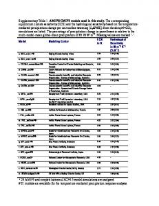
CMIP5 models used in this study: name, ocean vertical coordinate type (z, z*, isopycnic or sigma-level) and number of ocean vertical levels, average horizontal resolution (latitude x longitude), and reference. Only one number is indicated for the horizontal resolution if the latitude and longitude have the same resolution. Note that inmcm4 is not included in the multi-model analyses. * indicates models studied in the appendix (section 3.7). . . . . . . . . . . . . . . . . . . . . . . . . . . . . . . . . . . . . .

3.2

63

Historical (1986-2005) mean and temporal standard deviation of the annual mean over 1986-2100 (pre-industrial control run, not filtered) of the transports for the 25 models, and historical multimodel mean and spread: Atlantic Meridional Overturning Circulation (AMOC), Antarctic Circumpolar Current (ACC), Atlantic, Indian, Pacific and total bottom Southern Meridional Overturning Circulation (SMOC). The model inmcm4 is not included in the multimodel means as explained in the text. . . . . . . . .

xiii

78

3.3

Pacific Ocean, across-model correlations between the parameters “param” (σ stands for potential density, θ for potential temperature and S for salinity) for each latitude band “lat” and the transports: mean 1986-2005 historical value “hist”, mean 2081-2100 RCP8.5 value “RCP8.5”, and difference historical minus RCP8.5 minus pre-industrial control drift “change”. Only significant correlations (p-value < 0.05) are shown. The model inmcm4 was not included in the analysis. GISS-E2-H was removed from the transport changes because of its spurious pre-industrial run values. . .

85

3.4

Same as Table 3.3 for the Indian Ocean. . . . . . . . . . . . . . . . . . .

86

3.5

Same as Table 3.3 for the Atlantic Ocean. . . . . . . . . . . . . . . . . .

87

S1

Pacific Ocean (areas deeper than 3000 m), area-weighted mean change in bottom density and spatial standard deviation of this change (both in 10−3 kg m−3 ) per latitude band for each model, for RCP8.5. Longitude range in the south: 145◦ E to 295◦ E, in the north: 145◦ E to 250◦ E. Inmcm4 is not included in the multimodel mean. . . . . . . . . . . . . . . . . . . . 105

S2

Indian Ocean (areas deeper than 3000 m), area-weighted mean change in bottom density and spatial standard deviation of this change (both in 10−3 kg m−3 ) per latitude band for each model, for RCP8.5. Longitude range in the south: 25◦ E to 125◦ E, in the north: 55◦ E to 100◦ E. Inmcm4 is not included in the multimodel mean. . . . . . . . . . . . . . . . . . . . . . 106

S3

Atlantic Ocean (areas deeper than 3000 m), area-weighted mean change in bottom density and spatial standard deviation of this change (both in 10−3 kg m−3 ) per latitude band for each model, for RCP8.5. Longitude range in the south: 70◦ W to 25◦ E, in the north: 90◦ W to 0◦ E. Inmcm4 is not included in the multimodel mean. . . . . . . . . . . . . . . . . . . . 107

S4

For each model and the multimodel mean, correlation between the 19862100 timeseries in transport. ”-” indicates that the correlation was not significant. The letters corresponding to each model are indicated on figures 3-5; ”mm” stands for ”multimodel”. Inmcm4 is not included in the multimodel mean; correlation between its two non-zero transports AMOC and ACC = -0.44. . . . . . . . . . . . . . . . . . . . . . . . . . . . . . . 108

xiv

5.1

Sensitivity experiments performed at the Met Office on HadGEM3: “Langmuir” experiments look at Langmuir turbulence velocity scale, “Gamma” at the penetration of an additional turbulent kinetic energy term below the mixed layer, “Knoprof” and “KProf” at background diffusivity. “I” indicates that the parameter was increased compared to the default value, “D” that it was decreased. The run identifier is a pointer to the simulation name-list and configuration. The parameters column identifies the shorthand name used in the NEMO simulation name-list. The results of these experiments are presented in section 5.6. . . . . . . . . . . . . . . . . . . 135

xv

List of figures 1.1

Map of bottom neutral density in the Southern Ocean; AABW is represented by the shades of green. Red circles indicate the sites of AABW formation: (1) Weddell Sea, (2) Ross Sea, (3) Ad´elie Land and (4) Cape Darnley. Adapted from Orsi (2010). . . . . . . . . . . . . . . . . . . . .

1.2

2

Left: θ-S diagram (a) of Southern Ocean data used by Pardo et al. (2012) and (b) zoomed for bottom waters (WSBW, ADLBW and RSBW) and CDW, adapted from Pardo et al. (2012). Right: θ-S diagram and neutral density lines of the world ocean below 200 m depth divided into the three main ocean basins, adapted from Dietrich (1963). . . . . . . . . . . . . .

1.3

3

Schematic representation of shelf processes leading to the formation of AABW (highlighted in red). Numbers indicate the order of these processes, detailed in the text. Adapted from Smethie and Jacobs (2005). . .

1.4

5

Location of coastal polynyas around Antarctica, in grey, and the ice shelves next to which they form. Letters indicate open ocean polynyas: W for Weddell Polynya, M for Maud Rise and C for Cosmonaut Polynya. Dashed line is the maximum sea ice edge (Martin, 2001). . . . . . . . . . . . . .

1.5

6

Schematic flow pattern of AABW. Blue arrows indicate the shelf break current. Lilac hatching indicates the location of the Weddell and Ross

1.6

gyres. Adapted from Orsi et al. (1999). . . . . . . . . . . . . . . . . . . .

7

Fraction of AABW at ocean bottom, from Johnson (2008). . . . . . . . .

8

xvii

1.7

In the Southern Ocean south of 50◦ S, all locations occupied by a ship where at least one measurement has been taken deeper than 3000 m, at the date of the download (August 2014). The data were obtained from the World Ocean Database (http://www.nodc.noaa.gov/OC5/WOD/pr wod.html). In blue, measurements between 1874 and 2004; in red, since 2005. Grey contours indicate the 3000 m isobath. . . . . . . . . . . . . . . . . . . .

1.8

10

(left) Correlation and (right) regression between the seasonal mean SAM index and the seasonal mean ice concentration for the period 1980-1999 in the HadISST1 observations (Rayner et al., 2003) in summer (top) and winter (bottom). From Lefebvre et al. (2004). . . . . . . . . . . . . . . .

1.9

13

Composites of ice concentration anomalies (1982 to 1998) during two phases of SOI, after Kwok and Comiso (2002). . . . . . . . . . . . . . .

14

1.10 Schematic representation of the ESM IPSL-CM4. Each block represents a model component. Arrows highlight interactions between the components. Picture by M.A. Foujols for the BADC website (http://badc.nerc.ac.uk/). 17 1.11 Schematic summary of CMIP5 long-term experiments with tier 1 and tier 2 experiments organised around a central core. Green font indicates simulations to be performed only by models with carbon cycle representations. Experiments in the upper hemisphere are suitable either for comparison with observations or to provide projections, whereas those in the lower hemisphere are either idealised or diagnostic in nature and aim to provide a better understanding of the climate system and model behaviour (Taylor et al., 2012). . . . . . . . . . . . . . . . . . . . . . . . . . . . . . . . . .

18

1.12 Schematic representation of the CMIP5 experiments used in this thesis: piControl (yellow), historical (black), RCP4.5 (blue) and RCP8.5 (red). Green box indicates the 1986-2005 period of the historical run used in chapters 2, 4 and 5. Grey boxes indicate the 1986-2005 and 2081-2100 periods of all the runs, used in chapter 3. Adapted from Collins et al. (2013). 19

xviii

2.1

Mean bottom potential temperature of the climatology (a) and mean bottom temperature difference (model - climatology) (b-p); left colorbar corresponds to the climatology, right colorbar to the differences model-climatology (same unit). Thick dashed black line is the mean August sea ice extent (concentration>15%); thick continuous black line is the mean February sea ice extent (concentration>15%). Numbers indicate the area-weighted root mean square error for all bottom depths (shelf and deep ocean) between the model and the climatology (unit ◦ C); mean RMS = 0.97◦ C. . .

2.2

27

Mean bottom potential density σ2 of the climatology (a) and mean bottom density difference (model - climatology) (b-p); left colorbar corresponds to the climatology, right colorbar to the differences model-climatology (same unit). Thick black line is the maximum August MLD/bathymetry (quotient>50%); thin grey line is the 3000 m depth contour. Numbers indicate the area-weighted root mean square error for all bottom depths (shelf and deep ocean) between the model and the climatology (unit kg m−3 ); mean RMS = 0.18 kg m−3 . . . . . . . . . . . . . . . . . . . . . .

2.3

29

Mean bottom salinity of the climatology (a) and mean bottom salinity difference (model - climatology) (b-p) in August; left colorbar corresponds to the climatology, right colorbar to the differences model-climatology (same unit). Numbers indicate the area-weighted root mean square error for all bottom depths (shelf and deep ocean) between the model and the climatology (given on the practical salinity unit scale); mean RMS = 0.18. 38

2.4

Mean bottom salinity difference in the Southern Ocean (south of 63◦ S) for each model between August and February (August - February), on a logarithmic scale. Thick dashed black line is the mean August sea ice extent (concentration>15%); thick continuous black line is the mean February sea ice extent (concentration>15%). . . . . . . . . . . . . . . . . . . . .

2.5

40

Mean bottom density σ2 of (a) the climatology and (b)-(p) each model in August. Grey line indicates the 3000 m isobath. . . . . . . . . . . . . . .

xix

41

2.6

Southern Ocean south of 65◦ S, monthly sections of σθ (in kg m−3 ) from the shelf to the open ocean for the 11 models forming dense water on the shelf. Colorbars are non-linear to highlight the variations in the low densities. Model name, longitude and date are indicated on each panel. These dates and locations have been chosen to show the largest amount of dense water spilling off the shelf. All models are shown on the Ross Sea, but GFDL-ESM2G (b) which is in the Weddell Sea. . . . . . . . . . . . .

2.7

43

Southern Ocean south of 65◦ S, monthly anomalies of bottom σθ for HadGEM2ES from August 1997 to February 2000. The colorbar is non-linear to highlight the variations in the low anomalies. Grey plain contours indicate the 3000 m isobath; dashed grey contours indicate the 1000 m isobath. 44

2.8

Southern Ocean south of 65◦ S, monthly anomalies of bottom σθ for MIROCESM-CHEM from June 1993 to December 1995. The colorbar is nonlinear to highlight the variations in the low anomalies. Grey contours indicate the 3000 m isobath; dashed grey contours indicate the 1000 m isobath. . . . . . . . . . . . . . . . . . . . . . . . . . . . . . . . . . . .

2.9

46

Global map of the mean over all the monthly values from January 1986 to December 2005 of the bottom temperature (left) and bottom salinity (right) for CNRM-CM5 (a and b), CSIRO-Mk3-6-0 (c and d), NorESM1M (e and f) and INMCM4 (g and h). The colorscale is indicated in the centre between the temperature and salinity. On each map, grey lines indicate the 3000 m isobath. . . . . . . . . . . . . . . . . . . . . . . . . . . . . .

50

2.10 Maximum August mixed layer depth over the 20-yr of the study of Heuz´e et al. (2013), calculated for all the models using a σθ threshold of 0.03 kg m−3 . . . . . . . . . . . . . . . . . . . . . . . . . . . . . . . . . . . . . .

52

2.11 Maximum August mlotst over the 20-yr of the study of Heuz´e et al. (2013), for all the models for which this output was available. CSIROMk3-6-0 (d) has been made available only after the publication of Heuz´e et al. (2013), hence the discrepancy between the number of models in the text of the article and the ones presented here. . . . . . . . . . . . . . . .

xx

53

2.12 August maxima over the 20-yr of the study of Heuz´e et al. (2013) of our mixed layer depth (left), of mlotst re-computed following the CMIP5 recommended method (centre) and of the actual provided mlotst (right) for the three models for which these different methods give different results. 54 2.13 CanESM2, profile of temperature (left), salinity (centre) and density σθ (right) of a randomly selected point in the area where mlotst (red) and our mixed layer depth (black) give different results, i.e. in the Weddell Sea. The actual mixed layer depth is highlighted in green. . . . . . . . . . . .

55

2.14 MPI-ESM-LR, profile of temperature (left), salinity (centre) and density σθ (right) of a randomly selected point in the area where mlotst (red) and our mixed layer depth (black) give different results, i.e. in the Ross Sea. The actual mixed layer depth is highlighted in green. . . . . . . . . . . .

56

2.15 INMCM4, profile of temperature (left), salinity (centre) and density σθ (right) of a randomly selected point in the area where the provided mlotst (red) and our mixed layer depth (black) give different results, here in the Weddell Sea. The actual mixed layer depth is highlighted in green, and the mlotst we calculated using the method recommended by the CMIP5 documentation is in dashed red. . . . . . . . . . . . . . . . . . . . . . . . 3.1

57

Schematic depth/latitude section through the Atlantic Ocean of the meridional overturning circulation. Shading indicates oxygen content, that is time since the water was last ventilated (high oxygen / purple for areas of deep water formation). The two main water masses (AABW and NADW) and transports (ACC out of the page, SMOC and AMOC meridional) studied in this chapter are indicated. Adapted from Marshall and Speer (2012). 68

3.2

RCP8.5 multimodel mean change (2081 to 2100 minus 1986 to 2005) in a) bottom temperature, b) bottom salinity and c) bottom density σ2 . Control drift has been removed. Black stippling indicates areas where fewer than 16 models agree on the sign of the change. Grey contour indicates the 3000 m isobath. Yellow lines on the bottom panel indicate the study boundaries for the three ocean basins in the Southern Ocean. . . . . . . .

xxi

70

3.3

Observed winter mixed layer depth (shading) from the climatology of de Boyer Mont´egut et al. (2004) (updated in November 2008), calculated using a σθ threshold of 0.03 kg m−3 compared with 10 m depth, for a) the Southern Ocean south of 50◦ S and b) the North Atlantic. Black lines indicate the mean observed winter sea ice extent (plain line) and the mean observed summer sea ice extent (dashed line), from the HadiSST observations (Rayner et al., 2003). The three convective areas for section 3.4.4 are indicated by blue boxes on b): Labrador Sea (LA), Irminger and Iceland basins (II), and Norwegian and Greenland Seas (NG). Hatching in the LA and II boxes indicates the area used for the calculation of the mean profile changes in section 3.4.4 and Fig. 3.11. . . . . . . . . . . . . . . . . . . .

3.4

71

Southern Ocean, for each model, for each grid cell, historical (1986 to 2005) maximum depth of the mixed layer in any month of the twenty years. Black lines indicate the mean August sea ice extent (plain line) and the mean February sea ice extent (dashed line). . . . . . . . . . . . . . .

3.5

72

Southern Ocean, for each model, for each grid cell, RCP8.5 (2081 to 2100) maximum of the mixed layer in any month of the twenty years. Black lines indicate the mean August sea ice extent (plain line) and mean February sea ice extent (dashed line). . . . . . . . . . . . . . . . . . . . .

3.6

73

RCP8.5 bottom temperature change (2081 to 2100 minus 1986 to 2005) for each model, same scale for all 24 models. Control drift has been removed. Dark grey contour indicates the 3000 m isobath. . . . . . . . .

3.7

74

RCP8.5 bottom salinity change (2081 to 2100 minus 1986 to 2005) for each model, same scale for all 24 models. Control drift has been removed. Dark grey contour indicates the 3000 m isobath. . . . . . . . . . . . . . .

3.8

75

RCP8.5 bottom density change (2081 to 2100 minus 1986 to 2005) for each model, same scale for all 24 models. Control drift has been removed. Dark grey contour indicates the 3000 m isobath. . . . . . . . . . . . . . .

xxii

76

3.9

RCP8.5 time series of the change in transport from the 1986 value for each model after removal of the control drift and 15 year low-pass filtering: a) Atlantic Meridional Overturning Circulation at 30◦ N, b) Antarctic Circumpolar Current strength, c) Atlantic bottom Southern Meridional Overturning Circulation (SMOC) at 30◦ S, d) Indian SMOC, e) Pacific SMOC and f) sum of the SMOCs (total SMOC). For each panel, black line indicates the multimodel mean change. . . . . . . . . . . . . . . . .

79

3.10 Relationship between the change (2081 to 2100 minus 1986 to 2005) in each transport between RCP4.5 and RCP8.5: a) AMOC, b) ACC, c) Atlantic SMOC, d) Indian SMOC, e) Pacific SMOC, f) total SMOC. Control drift has been removed. For all the panels, the black diagonal line is the y = x line. . . . . . . . . . . . . . . . . . . . . . . . . . . . . . . . . . .

80

3.11 RCP8.5, change (2081 to 2100 minus 1986 to 2005) in the profile of a) temperature and b) salinity for each model (colours) and the multimodel mean (black) in the Labrador Sea. For each model, the profile displayed is the mean of the profiles over the area of the North Atlantic shown on Fig. 3.3 for the grid cells whose bathymetry is between 3200 and 3500 m.

88

3.12 North Atlantic, for each model, for each grid cell, historical (1986 to 2005) maximum depth of the mixed layer in any month of the twenty years. Black lines indicate the mean March sea ice extent (plain line) and the mean September sea ice extent (dashed line). . . . . . . . . . . . . .

90

3.13 North Atlantic, for each model, for each grid cell, RCP8.5 (2081 to 2100) maximum of the mixed layer in any month of the twenty years. Black lines indicate the mean March sea ice extent (plain line) and mean September sea ice extent (dashed line). . . . . . . . . . . . . . . . . . . . . . . .

91

3.14 North Atlantic (25 to 70◦ N, 280 to 360◦ E), for each model, RCP8.5 (20812100) mean actual bottom density σ2 . Stippling indicates where the change of bottom density is positive. Grey contour is the 3000 m isobath. . . . .

xxiii

92

3.15 HadGEM2-ES, Temperature-Salinity diagram of the bottom waters (deeper than 3000 m) of the Atlantic Ocean, shown as a function of latitude for the mean 1986-2005 of the historical run (top colorbar) and the mean 2081-2100 of RCP8.5. Large circles indicate the deep and bottom water formation areas (80 to 60◦ S, and 50 to 70◦ N), small crosses indicate the other latitudes. Black lines are the density σ4 contours. . . . . . . . . . .

93

3.16 Annual mean for 2006 to 2100, in RCP8.5 (red) and the pre-industrial control (black), of the AMOC (top), ACC (middle) and Pacific SMOC (bottom) for CanESM2 (respectively a, d and g), GFDL-ESM2G (b, e and h) and MIROC-ESM-CHEM (c, f and i). The period 2081-2100 studied in the text is shown in the grey box. . . . . . . . . . . . . . . . . . . . . 100 3.17 Annual mean for 2006 to 2100, in RCP8.5 (red) and the pre-industrial control (black), of the bottom potential temperature in the Atlantic between 80 and 60◦ S (top), of the bottom salinity in the Indian between 60 and 30◦ S (middle) and of the bottom potential temperature in the Pacific between 30 and 60◦ N (bottom) for CanESM2 (respectively a, d and g), GFDL-ESM2G (b, e and h) and MIROC-ESM-CHEM (c, f and i). The period 2081-2100 studied in the text is shown in the grey box. . . . . . . 101 3.18 Deep Southern Ocean (south of 50◦ S, bathymetry>3000 m), relationship between the area-weighted mean difference between models and climatology and 2081-2100 minus 1986-2005 minus drift (left), and relationship between the area-weighted RMS difference between model and climatology and 2081-2100 minus 1986-2005 minus drift (right) for the bottom potential temperature (a and b), salinity (c and d) and potential density σ2 (e and f). . . . . . . . . . . . . . . . . . . . . . . . . . . . . . . . . . . . 103

xxiv

S1

Figures for inmcm4 - see detailed captions of the main figures. Maximum MLD and mean sea ice extents in the Southern Ocean for a) the historical run and b) RCP8.5 (as in Fig. 3.3 and 3.4) ; c) bottom temperature change (as in Fig. 3.5), d) bottom salinity change (as in Fig. 3.6) and e) bottom density change (as in Fig. 3.7) ; f) AMOC and g) ACC timeseries for inmcm4 (red) and the multimodel mean shown on Fig. 3.8 (black); h) mean temperature and i) salinity change throughout the water column in the Labrador Sea for inmcm4 (red) and the multimodel mean shown on Fig. 3.10 (black); maximum MLD and mean sea ice extents in the North Atlantic for j) the historical run and k) RCP8.5 (as in Figs. 3.11 and 3.12); l) RCP8.5 mean 2081-2100 bottom density (as in Fig. 3.13). Apart from l), all figures are presented on the same scale as the corresponding figure in the text. . . . . . . . . . . . . . . . . . . . . . . . . . . . . . . . . . . 109

4.1

a) Mean January 1986 to December 2005 bottom density σ2 for the Southern Ocean south of 50◦ S and b) bathymetry of the region squared in blue on a). The three key regions for the OFP, given by Briegleb et al. (2010), are circled in black for the source (S), white for the interior (I) and dark grey for the entrainment (E). The pink line on b) indicates the location of the sections shown on Fig. 4.2. . . . . . . . . . . . . . . . . . . . . . . . 113

4.2

Monthly sections in the Ross Sea at the longitude 179◦ E of the density σθ (a and c) and the age of water (b and d) during an event of the OFP (November 2001, top) and two months later (January 2002, bottom). Note that the age of water is given on a logarithmic scale. On each panel, the source (S) and entrainment (E) regions are indicated by black and grey dotted lines respectively; the interior region (I) is not in this section. . . . 114

xxv

4.3

Same as Figs. 2.1, 2.2 and 2.3: mean bottom potential temperature (a), salinity (c) and potential density σ2 (e) of the climatology used in chapter 2 (Gouretski and Koltermann, 2004), and mean bottom temperature (b), salinity (d) and density (f) difference CCSM4-climatology. Thick dashed and continuous black lines on (a) and (b) represent the mean August and February sea ice extent respectively (sea ice concentration > 15%). Thick black line on (e) and (f) is the maximum August MLD/bathymetry (quotient>50%); thin grey line is the 3000 m isobath. See section 2.3 for the methods. . . . . . . . . . . . . . . . . . . . . . . . . . . . . . . . . . 116

4.4

Mean sea ice concentration between 1986 and 2005 for each month of CCSM4. Only the concentrations higher than 15% are shown for clarity. . 118

4.5

Sea ice concentration (greater than 15%) on the Ross shelf in January 2002. The regions from Fig. 4.1 are indicated again: black for the source, white for the interior, and dashed grey for the entrainment region. The pink cross shows the location of the exit point identified in section 4.2.1. . 119

4.6

Correlations between the sea ice concentration and a) the vertical water velocity at 100 m depth, b) the meridional water velocity at the surface and c) the surface wind speed. Black crosses indicate that the correlation is not significant (p-value > 0.05). The sea ice concentration lags one month behind the other field, i.e. correlations shown are for DJF for the sea ice concentration and NDJ for the other fields. Black contours indicate the mean February sea ice concentration = 15% line. . . . . . . . . . . . 120

4.7

Mean 1986-2005 meridional streamfunction for inmcm4 in the Atlantic Ocean (a) and monthly standard deviation of the streamfunction (b). The two main overturning cells have been schematically represented in black on (a). These results are shown on the regular grid provided for this output. 121

4.8

For each latitude-longitude grid cell in the Atlantic Ocean, (a) maximum through depth and time (1986-2005) of the density σ4 and (b) mean depth of the Weddell Sea bottom water isopycnal in inmcm4 (σ4 = 46.94 kg m−3 ). Results are shown interpolated on a regular grid of 1◦ x 1◦ instead of inmcm4’s native rotated grid. . . . . . . . . . . . . . . . . . . . . . . 122

xxvi

4.9

Mean 1986-2005 meridional streamfunction for inmcm4 in the Pacific Ocean (a) and monthly standard deviation of the streamfunction (b). The three main overturning cells have been schematically represented in black on (a). These results are shown on the regular grid provided for this output. 124

4.10 For each latitude-longitude grid cell in the North Pacific, a) maximum during 1986-2005 of the monthly mixed layer depth and b) bathymetry of the model inmcm4. Circles indicate the areas discussed in the text: the Sea of Japan (1), the Okhotsk Sea (2) and the eastern coast of the Kamchatka Peninsula in the Bering Sea (3). Grey contours on (a) indicate the 3000 m isobath. . . . . . . . . . . . . . . . . . . . . . . . . . . . . . 124 4.11 For each latitude-longitude grid cell in the Pacific Ocean, a) maximum through depth and time (1986-2005) of the density σ4 , and b) mean depth of the Ross Sea bottom water isopycnal in inmcm4 (σ4 = 47.09 kg m−3 ). Results are shown interpolated on a regular grid of 1◦ x 1◦ instead of inmcm4’s native rotated grid. . . . . . . . . . . . . . . . . . . . . . . . . 125 4.12 Depth of the isopycnal surfaces as a function of density σ4 and latitude (80◦ S to 30◦ N) for four longitudes: starting in East Antarctica east of the Kerguelen plateau (a, 94◦ E), on the Ross shelf (b, 177◦ W), in the Amundsen Sea (c, 119◦ W) and on the Weddell shelf (d, 32◦ W). . . . . . 126 4.13 Pre-industrial control run, difference August 2025 (red), 2080 (green) and 2100 (blue) minus August 1986 in density σ4 in the Argentine Basin (around 50◦ W and 45◦ S). a) is a theoretical profile showing erosion of the deep waters from the top at increasing depth levels through time, b) is a theoretical profile showing a linear drift of +0.62 10−3 kg m−3 yr−1 below 2000 m, and c) is the actual profile in inmcm4. . . . . . . . . . . . 127 5.1

Maximum monthly mixed layer depth reached between 1960 and 2005 for each latitude-longitude grid cell for (a) HadGEM2-ES and (b) HiGEM. Grey contour indicates the 3000 m isobath. . . . . . . . . . . . . . . . . 137

5.2

Yearly maximum area of open ocean deep convection from 1960 to 2005 for HadGEM2-ES (green) and HiGEM (blue). . . . . . . . . . . . . . . . 138

xxvii

5.3

For each year in the Southern Ocean, maximum monthly area of open ocean deep convection (red) from 1960 to 2005 for HadGEM2-ES (left) and HiGEM (right) compared with the annual minimum sea ice area (black, a and b), the annual maximum sea ice area (black, c and d), and the difference maximum - minimum (black, e and f). Note that in the Southern Ocean for each calendar year, the minimum occurs before the maximum; their difference gives an indication of how much sea ice was formed. . . . 140

5.4

For each year in the Southern Ocean, maximum monthly area of open ocean deep convection (red) from 1960 to 2005 for HadGEM2-ES (left) and HiGEM (right) compared with the annual mean SAM index (black, a and b) and the annual mean Ni˜no3.4 index (black, c and d). . . . . . . . . 142

5.5

NEMO with prescribed atmospheric forcing, default run, for each grid point, maximum monthly mixed layer depth between January 1980 and December 1989. The blue box indicates the Riiser-Larsen Sea region studied in section 5.4, which is overlaid by the dashed green box that indicates the Weddell Sea region studied in section 5.6. Grey contours indicate the 3000 m isobath. . . . . . . . . . . . . . . . . . . . . . . . . 143

5.6

Mechanisms leading to open ocean deep convection for the default run. . 144

5.7

Monthly anomalies in sea ice concentration relative to the period January 1980-December 1984 for the default run: a) May 1985 and b) June 1985. Black contours indicate the area where the maximum MLD from Fig. 5.5 is deeper than 2000 m. Grey contours indicate the 3000 m isobath. . . . . 145

5.8

Default run, a) median winter (July-November) MLD for 1980-1984 and monthly anomalies in MLD from July 1985 (b) to November 1985 (f). Left colorbar corresponds to the median MLD (a), right colorbar to the anomalies (b to f). Black thick contours indicate the area where the maximum MLD from Fig. 5.5 is deeper than 2000 m. Black stippling indicates that the anomaly is not significant (temporal standard deviation for 19801984 larger than the anomaly). Grey contours indicate the 3000 m isobath. 146

xxviii

5.9

a) Monthly temperature anomaly relative to 1980-1984 and b) profile of temperature from September 1985 to September 1987 over the area of the 1987 polynya. . . . . . . . . . . . . . . . . . . . . . . . . . . . . . . . . 147

5.10 Monthly sea ice concentration over the Riiser-Larsen Sea from June to November 1986 (a to f) and 1987 (g to l). Black contours indicate the area where the maximum MLD from Fig. 5.5 is deeper than 2000 m. Grey contours indicate the 3000 m isobath. . . . . . . . . . . . . . . . . 148 5.11 Default run, monthly mixed layer depth between a) August and c) October 1986, and between d) July and h) November 1987. Black contours indicate the area where the maximum MLD from Fig. 5.5 is deeper than 2000 m. Grey contours indicate the 3000 m isobath. . . . . . . . . . . . . 149 5.12 October 1986, a) monthly salinity anomaly relative to 1980-1984 at 21◦ E and b) profile of density σθ . Black (white) line on a) (b) indicates the monthly mixed layer depth. The black segment above each panel indicates the location of the 1987 polynya. . . . . . . . . . . . . . . . . . . . . . . 150 5.13 a) Monthly salinity anomaly relative to 1980-1984, b) density σθ shown as a difference from the surface value (on a logarithmic scale), c) profile of salinity and d) profile of density σθ from March 1986 to September 1987 over the area of the 1987 polynya. . . . . . . . . . . . . . . . . . . 151 5.14 Results from Calvert and Siddorn (2013): a) Mean annual cycle for 19821985 of biases in MLD averaged over the Southern Ocean (60◦ S-45◦ S) for their three cLC values; b) mean winter (black) and summer (red) biases in MLD averaged over the Southern Ocean (60◦ S-45◦ S) as a function of γ. On b), blue vertical line indicates the standard value of γ, and red and black dashed lines the bias in MLD in the configuration with no e¯inertial . Data courtesy of D. Calvert. . . . . . . . . . . . . . . . . . . . . . . . . 153 5.15 Weddell Sea, a) maximum monthly MLD ever reached between 1980 and 1989 by the default run and b) to h) difference maximum MLD of each simulation - maximum MLD of the default run. Left colorbar corresponds to a), right colorbar to b) to h). Grey contours indicate the 3000 m isobath. 155

xxix

5.16 Across-run significant relationships between the steps leading to the deep convection event of winter 1987. a) Sea surface temperature in June 1986 and polynya area in September 1986; b) polynya area and maximum depth of the mixed layer, both in September 1986; c) polynya area in September 1986 and surface salinity anomaly in February 1987; d) maximum depth of the mixed layer in September 1986 and sea surface temperature in February 1987; e) sea surface temperature in June 1987 and polynya area in October 1987; f) polynya area and maximum depth of the mixed layer, both in October 1987; g) polynya area and deep convection area, both in October 1987; h) surface salinity anomaly in February 1987 and maximum depth of the mixed layer in October 1987; i) surface salinity anomaly in February 1987 and deep convection area in October 1987. Horizontal (vertical) bars on a, e, h and i (c and d) indicate the spatial standard deviation. . . . . . . . . . . . . . . . . . . . . . . . . . . . . . 158 5.17 a) to h) Mixed layer depth in October 1987 for all the experiments, over the blue area of figure 5.5. MLD for the four experiments which have open ocean deep convection the following years in the green area of Fig. 5.5, in October 1988 (i to l) and October 1989 (m to p). For each panel, grey contours indicate the 3000 m isobath. . . . . . . . . . . . . . . . . . 159 5.18 Across-run relationships between the deep convection event in the RiiserLarsen Sea in 1987 and the subsequent deep convection event in the Weddell Gyre in 1988. a) Maximum depth of the mixed layer and b) area of deep convection, both in the Riiser-Larsen Sea in September 1987, compared with the Weddell Polynya area in September 1988 (presented on a log scale); c) maximum depth of the mixed layer and d) area of deep convection, both in the Riiser-Larsen Sea in September 1987, compared with the maximum MLD in the Weddell Gyre in September 1988. . . . . . . . 160

xxx

5.19 Run KnoprofD, Weddell Sea, a) 40 m depth speed (shading) and velocity vectors (black arrows) in February 1988; monthly temperature anomalies at 40 m depth relative to January 1980-December 1984 in b) October 1987, c) February 1988 and d) June 1988. Grey contours indicate the 3000 m isobath. Yellow (black) contours on a (b to d) indicate the areas of deep convection in 1987 (around 20◦ E) and 1988 (20◦ W). . . . . . . . 161 5.20 Weddell Sea, 1988-1989, a) difference between the mean bottom temperature in the default run and the climatology made of observations WOA13 (top left colorbar). b) to h) Difference in bottom temperature between each simulation and the default run (simulation - default, top right colorbar). i) Difference between the mean bottom salinity in the default run and the climatology made of observations WOA13 (bottom left colorbar). j) to p) Difference in bottom salinity between each simulation and the default run (simulation - default, bottom right colorbar). For b)-h) and j)-p), thick black contours indicate the area where the MLD represents at least 90% of the water column in 1987 and 1988; thin grey line indicates the 3000 m isobath. . . . . . . . . . . . . . . . . . . . . . . . . . . . . . . . 163 5.21 Weddell Sea, simulation Kprof, difference between the mean bottom temperature (a) and salinity (b) over 2003-2007 and 1988-1989. Thick black contour indicates where the 2000-2002 MLD represents at least 90% of the water column; thin grey line indicates the 3000 m isobath. . . . . . . 164 5.22 27 year time series of a), c) and e) monthly Atlantic SMOC (black) and monthly area of deep convection in the Weddell Sea (red); b), d) and f) annual maximum ACC (black) and annual maximum area of deep convection in the Southern Ocean (red). . . . . . . . . . . . . . . . . . . . . 166 5.23 North Atlantic, for each simulation, yearly maximum area of deep convection (same definition as chapter 3). . . . . . . . . . . . . . . . . . . . 168

xxxi

5.24 North Atlantic, for each latitude-longitude point, a) maximum MLD reached between January 1980 and December 1989 for the default run; b) to h) difference between the maximum MLD for each run and the default run maximum MLD. Top colorbar is for the default run, bottom colorbar for the difference plots. For each panel, grey contour indicate the 3000 m isobath. . . . . . . . . . . . . . . . . . . . . . . . . . . . . . . . . . . . 169

xxxii

Chapter 1

Introduction 1.1 1.1.1

Antarctic Bottom Waters Definition

In this thesis, we mainly focus on Antarctic Bottom Water (AABW): its characteristics, formation, variability, and role in climate in Global Coupled Models (GCMs). This water mass forms by sinking of the very cold waters on the Antarctic continental shelves. These cold waters then propagate northward, along the bottom of most of the world ocean. Antarctic Bottom Water accounts for more than a third of the mass of the global ocean (Johnson, 2008) and plays a key role in heat and possibly carbon storage (S´ef´erian et al., 2012). There are actually four types of bottom water, named after their formation area (red circles on Fig. 1.1): Weddell Sea Bottom Water (WSBW, Gill, 1973), Ross Sea Bottom Water (RSBW, Jacobs et al., 1970), Ad´elie Land Bottom Water (ALBW or ADLBW, Rintoul, 1998) and the Cape Darnley Bottom Water (CDBW), suspected by Wong et al. (1998) and recently observed by Ohshima et al. (2013). Definitions vary, particularly as these four locations do not have the same properties: RSBW is warmer and saltier than ALBW, itself warmer and saltier than WSBW (Fig. 1.2). CDBW has been discovered too recently to have a climatology of its characteristics. These different properties result in different densities in bottom waters lying in the deep basins of the Southern Ocean as can be observed on Fig. 1.1: the bottom of the Weddell Sea is filled with the densest water while the bottom of the Ross Sea is filled with the least dense water (less dense by at least

2

Introduction

Drake Passage

Weddell Sea

Bellinghausen Sea

Amundsen Sea Ross Sea

Oates Land

Figure 1.1: Map of bottom neutral density in the Southern Ocean; AABW is represented by the shades of green. Red circles indicate the sites of AABW formation: (1) Weddell Sea, (2) Ross Sea, (3) Ad´elie Land and (4) Cape Darnley. Adapted from Orsi (2010).

0.04 kg m−3 ). These four water masses also have common features. Their potential temperature is below 2◦ C no matter where they are formed (Fig. 1.2a) and therefore these waters are too cold to have been formed in the northern hemisphere (Fig. 1.2b: whichever ocean you consider, Antarctic bottom waters are the coldest). They also lie on the bottom of their

1.1 Antarctic Bottom Waters

(a) Southern Ocean

3

(b) World ocean

Figure 1.2: Left: θ-S diagram (a) of Southern Ocean data used by Pardo et al. (2012) and (b) zoomed for bottom waters (WSBW, ADLBW and RSBW) and CDW, adapted from Pardo et al. (2012). Right: θ-S diagram and neutral density lines of the world ocean below 200 m depth divided into the three main ocean basins, adapted from Dietrich (1963).

respective basin: as can be observed on Fig. 1.1, the deep basins next to the formation sites on the Antarctic shelves are filled with extremely dense water, with neutral densities 0.1 to 0.2 kg m−3 higher than the surrounding mid-latitude bottom waters. Finally, some of these bottom waters escape their basin to contribute to what is called Antarctic Bottom Water (AABW) and can be found at the bottom of the Pacific, Atlantic and Indian oceans (Fig. 1.2b). For these reasons, in this thesis, we study bottom waters as a whole and do not mention WSBW, ALBW, CDBW and RSBW but only call them “bottom water”.

1.1.2

Formation of Antarctic Bottom Waters

The importance of AABW’s propagation became obvious long ago. W¨ust (1933) noticed that the bottom of the Atlantic Ocean was filled with water coming from southern high latitudes. Deacon (1933) was the first to refer to this water mass as Antarctic Bottom Water. Sverdrup (1940) identified the differences between the mixed waters in the Antarctic Circumpolar Current (ACC) and the water masses they originate from, in the Southern Ocean. Foster and Carmack (1976) proposed a three stage formation process for AABW in the Weddell Sea (which can be followed on the Southern Ocean θ-S diagram of Fig. 1.2a and on Fig. 1.3): • Circumpolar Deep Water (CDW) with relatively high temperature and salinity, is modified by mixing with the overlying colder but less salty Winter Water, temperature minimum, remnant of the winter mixed layer (step 1 on Fig. 1.3);

4

Introduction

• modified CDW is carried westward in the southern limb of the Weddell Gyre and mixes with High Salinity Shelf Water (HSSW, near-freezing point and high salinity) and forms Weddell Sea Bottom Water (WSBW, step 2 on Fig. 1.3); • WSBW flows northward and mixes -again- with CDW to form AABW (step 3 on Fig. 1.3). This three stage formation process was later confirmed by tritium analyses (Michel, 1978) and geochemical tracers (Weiss et al., 1979). Despite some differences in salinity and temperature properties, the same mechanism is occurring for the Ross Sea Bottom Water and Ad´elie Land Bottom Water (Mantyla and Reid, 1983). Cape Darnley Bottom Water was identified too recently for the mechanism to be known for sure. The other process leading to the formation of AABW (illustrated on Fig. 1.3) begins with the formation of High Salinity Shelf Water (HSSW), a water mass created during sea ice formation (Foldvik et al., 2004). Adjacent to the Antarctic ice shelves, large and persistent open water areas contribute to HSSW formation: coastal polynyas (Drucker et al., 2011). In Antarctica, strong katabatic winds blowing from the continent push the ice away, opening coastal polynyas (see Fig. 1.4 for their location). The ocean is no longer protected by sea ice and undergoes a large heat loss to the atmosphere. The water surface temperature decreases until it reaches freezing point and sea ice is formed again. Because of brine rejection during sea ice formation, the cooled surface water also becomes saltier, hence extremely dense, and starts sinking to the bottom of the continental shelf (Talley, 1999). In the ice shelf cavity, because of the increased pressure, the freezing point is lower than at the surface. HSSW is relatively warm in comparison, and causes basal melting of the ice shelf, hence forming supercooled but less salty Ice Shelf Water (ISW, Gammelsrød et al., 1994). In the Weddell Sea, dense ISW will continue sinking to the bottom of the continental shelf and ultimately mix with the overlying Weddell Deep Water (WDW) to form WSBW (Foldvik et al., 2004). In the Ross Sea, ISW mixes with modified CDW, hence forming RSBW (Jacobs et al., 1970). Due to the scarcity of measurements close to the ice shelf in Southern winter, the exact process by which ISW forms bottom waters is unknown (Smethie and Jacobs, 2005). Then, this newly formed dense water will sink down the continental slope to fill the deep Antarctic basins and eventually escape northwards to the other oceans (Orsi et al., 1999).

1.1 Antarctic Bottom Waters

5

Figure 1.3: Schematic representation of shelf processes leading to the formation of AABW (highlighted in red). Numbers indicate the order of these processes, detailed in the text. Adapted from Smethie and Jacobs (2005).

In rare occasions, bottom water can be formed through open ocean deep convection (Killworth, 1983). In 1977, the Weddell Chimney was observed in the Weddell Gyre in summer. It is hypothesised that such a cold water chimney was a remnant of wintertime convection (Gordon and Huber, 1984). Hard to observe because of their small radius of 30 to 50 km (Killworth, 1979), Gordon and Huber (1984) suggest anyway that there may be 30 of these chimneys in the Weddell Gyre. These chimneys were accountable for less than 1 Sv of deep water formation; geochemical estimates suggest an AABW production between 8 and 15 Sv for the whole Southern Ocean (Doney and Hecht, 2002). The most important features of this deep convection are open ocean polynyas. The first one to be detected by remote sensing was the Weddell Polynya which opened from 1973 to 1976, but since then others have been observed (Fig. 1.4: Weddell, Maud Rise and Cosmonaut polynyas). In contrast with coastal polynyas, open ocean polynyas do not open because the wind blows the ice away, but because relatively warm water is being upwelled by the action of wind, melting the ice. Then due to the strong heat loss to the atmosphere, water is cooled and sinks to the bottom (Martinson et al., 1981). To date, there is no consensus as to what caused the Weddell Polynya to open only once since the late 1970s. This polynya and its representation in climate models will be the topic of chapter 5 of this thesis.

6

Introduction

Figure 1.4: Location of coastal polynyas around Antarctica, in grey, and the ice shelves next to which they form. Letters indicate open ocean polynyas: W for Weddell Polynya, M for Maud Rise and C for Cosmonaut Polynya. Dashed line is the maximum sea ice edge (Martin, 2001).

1.1.3

Circulation of Antarctic Bottom Water

In most of the Antarctic basins, newly formed bottom water flows down the continental slope from the shelf. This process is relatively quick: dense water stays on the shelf for a few days, and cascades to the open ocean at speeds exceeding 0.4 m s−1 (Foldvik et al., 2004; Williams et al., 2008). Newly formed bottom water then travels eastwards or westwards, following the shelf break current (Blue lines on Fig. 1.5): in the Ross Sea, RSBW extends towards the southeastern corner of the Australian-Antarctic basin; ALBW spreads from Ad´elie Land to 140◦ E; in the Amery Basin, young CDBW reaches 25◦ E; and in the Weddell Sea WSBW propagates to 30◦ E (Orsi et al., 1999). As can be observed on Fig. 1.5, in the southern Weddell Sea some of the water flows directly northward into the Atlantic basin through gaps in the bathymetry. Once it has spilled off the shelf and reached the open ocean, newly formed bottom water circulates in the subpolar gyres. In the northwestern part of the Weddell Sea, WSBW leaves the slope regime and flows cyclonically in the north of the Weddell Gyre (Orsi

1.1 Antarctic Bottom Waters

7

Weddell Gyre

Ross Gyre

Figure 1.5: Schematic flow pattern of AABW. Blue arrows indicate the shelf break current. Lilac hatching indicates the location of the Weddell and Ross gyres. Adapted from Orsi et al. (1999).

et al., 1993). Similarly, RSBW flows in the northern Ross Gyre (Orsi et al., 1999). CDBW flows cyclonically along the south and west of the Australian-Antarctic Basin (Mantyla and Reid, 1995). Some of these AABW then flow eastward with the Antarctic Circumpolar Current (ACC). Once it has reached the northeastern end of the Weddell Gyre, a portion of this AABW continues eastward as far as 60◦ E (Orsi et al., 1999). Most of it then spreads into the other main ocean basins (Fig. 1.5), after having spent up to 85 years at the bottom of the Southern Ocean (Stuiver et al., 1983). AABW (defined as having a potential temperature below 0◦ C) can be found on the bottom of the three main ocean basins (Fig. 1.6). About 60% of the newly formed Antarctic Bottom Water enters the Atlantic sector (about 6 Sv, Orsi et al., 2001). While it covers more than 90% of the ocean bottom in the deep Antarctic basins and 60% in the Brazil basin, its fraction decreases with its northward path. This water mass represents only 20%

8

Introduction

Figure 1.6: Fraction of AABW at ocean bottom, from Johnson (2008).

of the ocean bottom north of the equator and less than 10% north of 35◦ N where the North Atlantic Deep Water dominates. The equivalent thicknesses of the AABW layer obtained by Johnson (2008) vary from 4000 m in the deep Weddell Basin where it is formed, to more than 1000 m in the equatorial Brazil basin and thinning to 250 m by 30◦ N (Johnson, 2008). The AABW which does not enter the Atlantic sector (40% of all the newly formed AABW) spreads in the Indian and Pacific Oceans (respectively 6 and 10 Sv, see for example Kouketsu et al., 2011). The deep Indian Ocean is filled by bottom water coming predominantly from the Weddell Gyre through the ACC (Mantyla and Reid, 1995). AABW represents more than 70% of all the water masses on the bottom of the Indian Ocean until north of the equator, and still accounts for 50% of all the water masses until the very north of the deep Arabian Sea (Johnson, 2008). Finally, due to its high density, most of the AABW from the Weddell Sea cannot cross Drake Passage towards the Pacific Ocean. Only the small modified, lighter, fraction can rise from the bottom to its 4000 m depth. Hence the Pacific basin is filled mainly with bottom water from the Ross Gyre (Orsi et al., 1999). As in the Indian Ocean, AABW fills much of the deep Pacific, with more than 70% of the bottom water masses being AABW until the equator and 60% all the way to the Aleutian Islands. In both the Indian and Pacific basins, this fraction is equivalent to a thickness of 1000 to 2000 m everywhere in

1.1 Antarctic Bottom Waters

9

the deep basins (Johnson, 2008).

1.1.4

Observations of Antarctic Bottom Water and climatologies used in this thesis

In this thesis, we focus on waters of the Southern Ocean deeper than 3000 m. That is 1000 m too deep for the current generation of Argo floats and gliders. Hence observations of Antarctic bottom waters rely on ship-based measurements. The World Ocean Database (http://www.nodc.noaa.gov/OC5/WOD/pr wod.html) gathers all the oceanic measurements performed since January 1773. In the Southern Ocean south of 50◦ S, it has just above 10,000 casts deeper than 3000 m, starting with the Challenger expedition of 1874 (Fig. 1.7). For comparison, over 1874-2014, about 300,000 ship-based casts have been performed in the North Sea. The deep Southern Ocean is poor in observations, in particular outside of the Weddell Sea (see Fig. 1.7 around the Kerguelens or in the Pacific sector), but all large areas have been occupied at least once. There is not enough data to study centennial trends in water properties, but there is enough to build climatologies. The HadiSST climatology (Rayner et al., 2003), used to assess the performances of the Hadley Centre models, cannot be used in this thesis: it is satellite-based, and gives only the surface properties of the ocean. Likewise, the new climatology MIMOC (Schmidtko et al., 2013) is not useful for us: it relies largely on Argo data and does not extend below 1925 m. In this thesis, we use two other climatologies: the Gouretski and Koltermann (2004) climatology in chapter 2, and the World Ocean Atlas 2013 (WOA2013, Locarnini et al., 2013; Zweng et al., 2013) in chapter 5. In chapter 2, we focus on climate models for whom “present-day” means end of the historical run (2005), hence we compare them with a climatology from 2004. In chapter 5 however we work on HadGEM3, a model which is still in development, hence we use the most up-to-date climatology.

10

Introduction

Figure 1.7: In the Southern Ocean south of 50◦ S, all locations occupied by a ship where at least one measurement has been taken deeper than 3000 m, at the date of the download (August 2014). The data were obtained from the World Ocean Database (http://www.nodc.noaa.gov/OC5/WOD/pr wod.html). In blue, measurements between 1874 and 2004; in red, since 2005. Grey contours indicate the 3000 m isobath.

1.1 Antarctic Bottom Waters

11

There is a small difference between these climatologies, probably because WOA2013 contains 1700 more casts than the Gouretski and Koltermann (2004) climatology (red dots on Fig. 1.7). On average over the deep Southern Ocean (deeper than 3000 m), the Gouretski and Koltermann (2004) climatology is 0.6◦ C colder and 0.001 fresher than WOA2013 at the bottom of the ocean. At the surface, it is colder and saltier than the austral summer (hereafter and throughout the thesis referred to only as “summer”) WOA2013 climatology (-0.6◦ C and 0.063) and warmer and fresher than the austral winter (hereafter and throughout the thesis referred to only as “winter”) WOA2013 climatology (0.9◦ C and -0.039). As the climatologies are not used in the same chapter to compare the same things, these differences are not further studied.

1.1.5

Modes of variability of the Southern Ocean

To date, there are very few studies based on observations that highlight a direct link between AABW and the modes of interannual variability of the Southern Ocean – El Ni˜no Southern Oscillation (ENSO) and the Southern Annular Mode (SAM). For instance, Jullion et al. (2010) suggest that the recent positive trend in SAM may be responsible for a warming of AABW in the Atlantic sector while L’Heureux and Thompson (2006) found that ENSO mainly enhances the consequences of SAM in the Southern Ocean rather than impacting the Southern Ocean directly. Other authors tried looking at these modes and their relationship with bottom water characteristics or formation in simple models, but they are not sure they captured the whole phenomenon, mainly because timeseries of deep data are not long enough to compare model results with observations (e.g. Timmerman et al., 2002). However, recent studies have succeeded in correlating sea ice – which plays a key role in AABW formation as explained in section 1.1.2 – interannual variability with these modes (e.g. Kwok and Comiso, 2002; Lefebvre et al., 2004; Stammerjohn et al., 2008; Cheon et al., 2014). Their findings are detailed in the following paragraphs.

Southern Annular Mode

The Southern Annular Mode (SAM) as defined by Thompson

and Wallace (2000) is the leading principal component of the sea level pressure (SLP, or of the 850 hPa geopotential height) anomalies south of 20◦ S. When the SAM is in a positive phase, there are low SLP anomalies at high latitudes and high SLP anomalies at low latitudes, leading to a poleward shift of the westerly winds (Thompson and Wallace,

12

Introduction

2000). The SAM is the dominant mode of variability of the Southern Hemisphere, and exhibits variabilities from weeks to years (Sall´ee et al., 2010). The influence of SAM on sea ice results in a dipole pattern (Fig. 1.8): during positive SAM years, the sea ice area decreases in the Weddell and Bellingshausen Seas but increases in the Ross and Amundsen Seas (Lefebvre et al., 2004). The SAM also seems to be correlated with sea ice growth, a positive SAM resulting in a delayed sea ice advance, but not significantly with sea ice decrease (Stammerjohn et al., 2008). SAM has also been linked with the opening of the Weddell Polynya. Gordon et al. (2007) hypothesise that the Weddell Sea became freshwater–depleted because of a decade of negative SAM. As the surface water salinity increased, the water column became unstable, ultimately causing open ocean deep convection. In contrast, Cheon et al. (2014) found that it is not the duration of the negative SAM phase but the sudden change to a positive phase, and its associated increase in westerly winds, which triggered the Weddell Polynya opening.

˜ - Southern Oscillation The El Ni˜no phase is defined by the World MeteoroEl Nino logical Organization as a positive anomaly in the eastern equatorial Pacific of sea surface temperature (SST), usually followed by a cold anomaly event called La Ni˜na(WMO, 1992). Both El Ni˜noand La Ni˜naare accompanied by atmospheric pressure changes between the east and west Pacific; that is the Southern Oscillation. These atmospheric and oceanic changes follow an irregular cycle (period of 2-7 years) called the ENSO cycle. They are represented by the Southern Oscillation Index (SOI), defined as the normalised SLP difference between Tahiti, French Polynesia, and Darwin, Australia (WMO, 1992). A negative SOI corresponds to El Ni˜no, a positive SOI to La Ni˜na. ENSO is most strongly correlated to sea ice in the Ross, Amundsen and Bellingshausen Seas. A positive SOI leads to an increase in both sea ice extent and sea ice concentration in the Ross and Amundsen Seas, and a decrease in the Weddell and Bellingshausen Seas (Fig. 1.9). It however shortens the sea ice season in the eastern Ross, Amundsen and western Weddell Seas, while increasing its length in the western Ross, Bellinghausen and central Weddell Seas (Kwok and Comiso, 2002). In the particular area of the Weddell Sea where the polynya opened in the late 1970s, a positive SOI (La Ni˜na) increases the sea ice formation and hence brine rejection; Gordon et al. (2007) suggest that the positive

1.1 Antarctic Bottom Waters

13

Figure 1.8: (left) Correlation and (right) regression between the seasonal mean SAM index and the seasonal mean ice concentration for the period 1980-1999 in the HadISST1 observations (Rayner et al., 2003) in summer (top) and winter (bottom). From Lefebvre et al. (2004).

SOI phase during the Weddell Polynya opening may have further destabilised the water column and triggered deep convection. There are also complex teleconnections between SAM and ENSO in some parts of the Southern Ocean. Stammerjohn et al. (2008) found that during years of both positive SAM and La Ni˜na event (positive SOI), sea ice retreats earlier in spring and advances later the following autumn in the Bellinghausen Sea, while in the western Ross Sea sea ice retreats later in spring and grows earlier the following autumn. The opposite behaviour is observed in the same regions when both SAM and SOI are negative (El Ni˜no event). Their results were not significant for the other areas of the Southern Ocean.

1.1.6

Observations of changes

AABW formation is not a steady process and bottom water properties may be already changing. Broecker et al. (1999) argued that only 4 Sv on average of bottom water have been produced annually over the past 100 years whereas the production rate over the past

14

Introduction

Figure 1.9: Composites of ice concentration anomalies (1982 to 1998) during two phases of SOI, after Kwok and Comiso (2002).

800 years was 15 Sv on average. They suggest that this difference may be due to a natural 1500 year long cycle in bottom water production. Likewise, Latif et al. (2013) suggest a centennial cycle in AABW formation, with high production phases exhibiting open ocean deep convection (which would then have stopped in the late 1970s) and low production phases where AABW is formed by shelf processes (like nowadays). The decrease in AABW formation might also be linked to both global warming and the increasing sea ice extent. Bintanja et al. (2013) highlighted that Antarctic ice shelf melting, due to the warming of Circumpolar Deep Water, creates a relatively fresh layer around Antarctica, facilitating sea ice formation by strongly reducing mixing. Lavergne et al. (2014) further suggested that this fresh layer makes it unlikely that AABW will be formed by open ocean deep convection again, as the salinity stratification increases. There are also rapid changes in the bottom water that have been observed recently: deep Antarctic waters are freshening (Bindoff and Hobbs, 2013) and warming (Purkey and Johnson, 2010). Throughout the Australian-Antarctic basin, AABW is rapidly freshening and hence becoming less dense, probably because of the changes in high latitude freshwater balance (Rintoul, 2007), especially the melting of glaciers in the Amundsen Sea (Bindoff and Hobbs, 2013). Similar observations have been made in the South Atlantic Ocean, where bottom water freshened and became less dense (Coles et al., 1996).

1.1 Antarctic Bottom Waters

15

Closer to the source, Jullion et al. (2013) found that AABW in the Weddell Sea is freshening in response to the melting of ice-shelves of the eastern side of the Antarctic Peninsula, while Hellmer et al. (2011) suspect that the freshening of Weddell Sea shelf waters are caused by an increase in precipitation and sea ice retreat. Throughout the bottom of the Pacific Ocean a warming has been detected since the 1990s, the largest signal being found in the south where bottom water forms. This warming may be due to the heat gain of the upper layers of the ocean over the past decades (Johnson et al., 2007). More importantly, this recent warming and freshening signal is spreading towards the equator and can already be detected in the tropical Pacific (Purkey and Johnson, 2013). In summary, despite the limited length of the observation time series, it seems that AABW is already reacting to climate change. Hence studying its representation in climate models is relevant: one would expect to see changes in models’ AABW properties in a timescale of a few decades (that will be the topic of chapter 3). In addition, AABW is not only passively subjected to climate change: it plays a role in the global climate system. AABW is important for climate regulation because it stores heat. Heat content of AABW from the equatorial Pacific has increased by 0.06 W m−2 between 1992 and 2003, which accounts for 10% of the heating trend estimated for the top 750 m of the world ocean over the same period (Johnson et al., 2007). An increasing trend has also been observed in the South Atlantic (Johnson and Doney, 2006). Durack et al. (2014) recently showed that these trends are likely to be biased low in the Southern Hemisphere mainly, because of the lack of measurements and limitations in previous analysis methods. Hitherto because of the sparsity of measurements in the deep Southern Ocean no estimation has been made regarding the heat storage of bottom waters around Antarctica, yet Johnson et al. (2007) believe that changes observed in the world ocean bottom waters are reflective of similar changes occurring closer to their Antarctic shelf formation sites. AABW plays little role in carbon storage, due to its very high Revelle factor (ratio between the solubility and the biological pump, indicates how efficient the reaction of atmospheric CO2 with seawater is), its limited contact with the surface, and sea ice acting as a physical barrier to CO2 uptake (Sabine et al., 2004). Finally, AABW formation is one of the drivers of the global thermohaline circulation.

16

Introduction

The principle of conservation of mass applied to the whole ocean means that any downwelling must be balanced by an equivalent upwelling. Hence bottom water formation by sinking of dense water induces upwelling in the Indian and Pacific oceans, keeping the Southern Ocean convection cells active (Sloyan and Rintoul, 2001). AABW formation and circulation is also the precursor of water mass flows and conversions (Schmitz, 1995).

1.2 1.2.1

Global Climate Models Basic description of Global Climate Models

In this thesis, we focus only on Global Coupled Models / Global Climate Models / General Circulation Models (GCMs) which aim at representing the whole climate system and its interactions, for the whole world. GCMs are based on fundamental laws of physics (mass, energy and momentum conservations), expressed in mathematical terms and implemented on computer after numerical discretisation or parameterisation. The GCMs used in the thesis belong to two different categories: the Atmosphere-Ocean General Circulation Models (AOGCMs) and the Earth System Models (ESMs). AOGCMs are the purely physical models that have been used in all previous Climate Model Intercomparison Projects (CMIP). They aim at representing the interactions between only the physical components of the climate system (atmosphere, ocean, sea ice and land). ESMs are generally built on AOGCMs but also include some biogeochemical cycles such as the carbon cyle, the sulphur cycle, or ozone (Flato, 2011). AOGCMs and ESMs both have the same skeleton: several model components (e.g. an ocean model, an atmospheric model, a sea ice model and a land model) linked together with conservative coupling. The relationships between various aspects of the components are schematically represented in Figure 1.10: in the case of an ESM, not only do the physics of the components interact, but there are also interactions physicsbiogeochemistry (e.g. greenhouse gases and atmospheric circulation) and biogeochemistrybiogochemistry (between the ocean and the atmosphere for instance). For all GCMS, the forcings are of two types (Flato et al., 2013): natural (solar radiation and volcanic eruptions) and anthropogenic (e.g. greenhouse gases and aerosols emissions, land use change).

1.2 Global Climate Models

17

Figure 1.10: Schematic representation of the ESM IPSL-CM4. Each block represents a model component. Arrows highlight interactions between the components. Picture by M.A. Foujols for the BADC website (http://badc.nerc.ac.uk/).

Within each component a distinction is made between what can be represented in the model, called the dynamical core, and sub-gridbox processes that cannot be represented and need to be parameterised (e.g. tropical cloud convection, small scale eddies, melt ponds on sea ice...). This distinction depends on characteristics of the GCM such as its resolution, as well as computational resources available to the modelling centre and the relative importance given to each process (Flato et al., 2013) and will vary from one model to another. For instance, most models used in this thesis have a resolution of about 1◦ in the ocean and have parameterised eddies, but two models have a higher resolution of 1/3◦ (HiGEM) or even locally 1/4◦ (MIROC4h) and are eddy-permitting. GCMs also differ in their horizontal grid type (regular, rotated or tripolar) and in their ocean vertical grid system (in this thesis, models are mostly on z-level grids, but we also use two hybrid/isopycnal and four σ-level models). With so many differences in their structure, GCMs developed by different centres provide different or even contradictory results to the same question (Cess et al., 1989). It became obvious nearly 20 years ago that a common framework was needed, and in 1995 the first CMIP was established (Meehl et al., 2000).

18

Introduction

Figure 1.11: Schematic summary of CMIP5 long-term experiments with tier 1 and tier 2 experiments organised around a central core. Green font indicates simulations to be performed only by models with carbon cycle representations. Experiments in the upper hemisphere are suitable either for comparison with observations or to provide projections, whereas those in the lower hemisphere are either idealised or diagnostic in nature and aim to provide a better understanding of the climate system and model behaviour (Taylor et al., 2012).

1.2.2

CMIP5 and what to do with a GCM

The fifth phase of the Climate Model Intercomparison Project (CMIP5) is an international collaboration providing a multimodel context to try to understand why similarly forced models produce a range of responses (Taylor et al., 2012). It is a platform for scientists to get climate outputs that can easily be compared in order to increase our understanding of the climate system and narrow the uncertainties regarding future climate predictions (IPCC, 2013). To do so, a wide range of experiments was designed and split into three “tiers” (Fig. 1.11): the core experiments (centre, pink) are critical for climate change predictions as well as understanding model differences, whereas tier 1 (middle, yellow) and tier 2 (outer ring, green) examine specific aspects of climate model forcing, processes and response, with tier 2 being even more specialised than tier 1 (information about each experiment is given by Taylor et al., 2012).

1.2 Global Climate Models

19

piControl historical

RCP4.5 RCP8.5

8 Figure 1.12: Schematic representation of the CMIP5 experiments used in this thesis: piControl (yellow), historical (black), RCP4.5 (blue) and RCP8.5 (red). Green box indicates the 1986-2005 period of the historical run used in chapters 2, 4 and 5. Grey boxes indicate the 1986-2005 and 2081-2100 periods of all the runs, used in chapter 3. Adapted from Collins et al. (2013).

In this thesis we focus on the core experiments of the upper hemisphere (Fig. 1.11) designed for comparison with observations and climate predictions: historical (black line on Fig. 1.12), pre-industrial control (piControl, yellow line on Fig. 1.12), Representative Concentration Pathway (RCP) 4.5 and RCP8.5 (blue and red lines on Fig. 1.12 respectively). Their full description is provided by Taylor et al. (2012) – we here only provide some key characteristics. In the historical experiment (1850-2005), forcings change with time and depend on observations (solar cycle, volcanic eruptions, greenhouse gas concentration). The piControl run consists of 500 years after the model has spun-up; forcings are prescribed and constant at a pre-industrial control level, allowing us to measure the internal variability of the model. RCP4.5 and RCP8.5 are climate change scenarios, corresponding to an imbalance in the Earth radiative budget of respectively 4.5 W m−2 and 8.5 W m−2 by 2100 (van Vuuren et al., 2011). In the IPCC Assessment Report 5 (AR5), the CMIP5 historical and piControl experiments are used to assess the performances of GCMs, compared with observations or other

20

Introduction

models (Flato et al., 2013), while the RCP experiments are used to predict future climate change and sea-level rise (Collins et al., 2013). CMIP5 models are also compared with the previous generation of CMIP3 models to observe the evolution of models: the model spread has decreased, but not drastically, despite a strong effort in increasing the resolution and number of processes which are resolved. AR5 is also the first report to include process-based assessments of GCMs, highlighting problems in the physics of the models that model developers might want to solve for the next CMIP (Flato et al., 2013).

1.2.3

Some limitations of CMIP5 models to bear in mind while reading this thesis

The content of the dynamical core of a GCM depends among other things on its resolution. Hence some key processes in the real ocean cannot be represented in the models we are using (e.g. dense water overflows, see chapter 2). We then need to discover what the model is doing instead to obtain an equivalent result (e.g. Southern Ocean deep convection). Some real processes are still not fully understood either, mainly because of a lack of observations (especially true for the deep ocean and high latitudes). Hence, it is not always possible to directly compare a GCM with observations. Another issue is the compromise model developers have to make regarding computer resources, and especially storage space. To save space, some fields are not stored. This choice is left at the discretion of model developers, resulting in specific fields being available for some models but not for all of the ones selected for our study (see chapter 2 the example of mlotst, chapter 3 the Bolus velocity and chapter 4 the tracers). It also happens that climate centres decide not follow the recommendations of CMIP5, and will provide their outputs on a different coordinate system or calculate their results with other formulae without warning the users (see the example of inmcm4, chapters 2 to 4). It is then up to the researcher to discover that the model developers have used a different scheme and to account for it. Finally, one should not forget that models can be tuned to match observed climate system behaviour (Flato et al., 2013). As a consequence, they are limited by our knowledge of the climate system and the lack of observations, and cannot take into account phenomena that we do not understand yet (like the present increase of Antarctic sea ice).

1.3 This thesis: research interest and aims

21

The performance of a GCM regarding the present-state of the climate cannot give clues about its ability to predict future climate change. A model which poorly represents the present-state will enter the climate change simulations with an ill-depicted initial state and so is unlikely to provide a feasible depiction of the future climate state. We do not know if we can have confidence in a model whose present-state is relatively accurate either.

1.3

This thesis: research interest and aims

In this thesis, we focus on Antarctic Bottom Water. To our knowledge there has been no assessment of AABW in the previous generation of climate models (CMIP3). In CMIP5, apart from this thesis only Sall´ee et al. (2013b) looked at Southern Ocean water masses -including AABW- in models, but AABW is the one they less thoroughly studied as they were not that confident in their method to detect it (J-B. Sall´ee, personal communication in May 2012). The first part of this thesis (chapter 2) assesses CMIP5 models’ performances regarding bottom water characteristics in the Southern Ocean. Historical biases are estimated for each model of our sample by comparing the present-state of their Southern Ocean with a climatology made of observations. We then explain these biases through a process-based study. We (re)discover that models cannot represent Antarctic shelf processes and hence form their bottom water through another process: open ocean deep convection. We investigate how present-day inaccuracies, both in bottom water characteristics and formation processes in CMIP5 models, affect future climate projections. In chapter 3, we assess the changes in bottom water properties globally in CMIP5 models under two climate change scenarios: RCP4.5 (moderate warming) and RCP8.5 (strong warming). We study the processes that control the magnitude and equatorward extent of the changes in bottom properties, as well as the consequences of said changes. In particular, the impact of bottom water changes on future sea level rise is estimated and compared with the current steric sea level rise due to the observed warming of bottom waters found by Purkey and Johnson (2013) as well as that projected by the IPCC AR5 (Collins et al., 2013). We conclude the CMIP5 study with a brief chapter (chapter 4) focusing on two models: CCSM4 and inmcm4. CCSM4 features a possible solution to represent dense water

22

Introduction

overflows from the Antarctic shelf to the open Ross and Weddell Seas. We assess the Southern Ocean bottom water properties of this model, as well as possible issues caused by this artificial overflow. We also investigate where AABW comes from in inmcm4, a puzzling model that has been a strong outlier in both chapter 2 and 3 as well as in other people’s CMIP5 studies (e.g. Meijers et al., 2012; Sall´ee et al., 2013b). As open ocean deep convection in the Southern Ocean proved key in all the previous chapters, in chapter 5 we try to understand which phenomena trigger open ocean deep convection in GCMs. To do so, we focus on the UK family of climate models: HadGEM2ES and HiGEM from CMIP5, as well as the new model HadGEM3. After a study of their outputs proves unsuccessful to clearly determine what is responsible for causing open ocean deep convection in models, a set of sensitivity experiments is designed and performed on HadGEM3 at the UK Met Office. We identify the chain of events leading to Southern Ocean open ocean deep convection. The sensitivity experiments investigate the effects of increasing or decreasing three mixing parameters on Southern Ocean deep convection, ocean circulation and North Atlantic deep convection. Chapter 6 contains a brief summary of our findings and a discussion of the limitations of our study. Ways that climate models can improve for the upcoming CMIP6 are presented, some of which are already under development and some others that seem feasible according to our findings. Particular attention is given to the processes that we found to be key for accurate steric sea level rise projections and those that would impact glacier and ice sheet melting.

Chapter 2

Southern Ocean bottom water characteristics in CMIP5 models Preamble This study has been published in Geophysical Research Letters in April 2013 with the same title by C´eline Heuz´e, Karen J. Heywood, David P. Stevens and Jeff K. Ridley, and will be hereafter referred to as Heuz´e et al. (2013). The text in this chapter is unchanged compared with the article apart from minor spelling and references to figures which are not shown in the paper due to space limitation but are provided in in the supplementary material section at the end of this chapter (section 2.6). The work has been done mostly by CH, under the supervision of KJH and DPS at the University of East Anglia, and JKR at the UK Met Office.

2.1

Abstract

Southern Ocean deep water properties and formation processes in climate models are indicative of their capability to simulate future climate, heat and carbon uptake, and sea level rise. Southern Ocean temperature and density averaged over 1986-2005 from fifteen CMIP5 climate models are compared with an observed climatology, focusing on bottom water. Bottom properties are reasonably accurate for half the models. Ten models create dense water on the Antarctic shelf, but it mixes with lighter water and is not exported as bottom water as in reality. Instead most models create deep water by open ocean deep convection, a process occurring rarely in reality. Models with extensive deep convection are those with strong seasonality in sea ice. Optimum bottom properties occur in models

24

Southern Ocean bottom water characteristics in CMIP5 models

with deep convection in the Weddell and Ross Gyres. Bottom Water formation processes are poorly represented in ocean models and are a key challenge for improving climate predictions.

2.2

Introduction

The Southern Ocean plays a key role in regulating the Earth’s climate: it connects the three main ocean basins, transporting heat and carbon (S´ef´erian et al., 2012), and its sea ice greatly affects the planetary albedo. Bottom water formed in the Southern Ocean circulates worldwide (Orsi et al., 1999). Numerous Global Climate Models (GCMs), with different parameterisations, resolutions and structures, are being used by scientists worldwide to estimate the likely climate in 50-100 years (e.g. global temperature increase or sea level rise). The ability of a model to adequately depict bottom water formation is crucial for accurate prediction of changes in the thermohaline circulation (Hay, 1993). In the real ocean, Antarctic Bottom Water usually forms when cold dense water spills off the shelf (Orsi et al., 1999), and then spreads northwards. This process is particularly challenging to represent in the current generation of climate models. There have also been episodes of open ocean deep convection, mostly observed in the Weddell Sea in the 1970’s (Killworth, 1983). Here we assess how dense water is formed in climate models, and how this impacts the representation of ocean properties at the sea bed. The CMIP5 project (Taylor et al., 2012) facilitates assessment of the models’ ability to depict the present observed state of the climate system, a prerequisite for reliable future prediction. Southern Ocean observational data coverage has dramatically increased over recent decades, particularly in the ice-free regions, enabling a detailed analysis of climate model simulations of this key region. The last generation of models in CMIP3 poorly represented Southern Ocean transport and heat fluxes (Russell et al., 2006). Subantarctic Mode Water and Antarctic Intermediate Water layer thicknesses and northward extensions were too small, despite a reasonably accurate depiction of temperature and salinity (Sloyan and Kamenkovitch, 2007). To our knowledge, there has been no assessment of Antarctic Bottom Water in CMIP3 models. Here we evaluate bottom water properties in the Southern Ocean in CMIP5 models.

2.3 Methodology

2.3

25

Methodology

We assess Southern Ocean potential temperature, salinity, density and sea ice concentration in fifteen CMIP5 historical simulations (means of the twenty August monthly mean fields from 1986 to 2005, of the first ensemble member, designated r1i1p1 in PCMDI terminology). The models include a hybrid/isopycnal model: GFDL-ESM2G (Dunne et al., 2012), available through CMIP5 on z-level coordinates, and three σ-coordinate models: INMCM4 (Volodin et al., 2010) requiring conversion to z-coordinates, MIROC4h (Sakamoto et al., 2012) and MIROC-ESM-CHEM (Watanabe et al., 2011), both available converted to z-level coordinates. The remaining 11 are traditional z-level models: CanESM2 (Chylek et al., 2011), CNRM-CM5 (Voldoire et al., 2011), CSIRO-Mk3-6-0 (Gordon et al., 2010), GFDL-ESM2M (Dunne et al., 2012), GISS-E2-R (Schmidt et al., 2006), HadGEM2-ES (Jones et al., 2011), HiGEM (Shaffrey et al., 2009), IPSL-CM5ALR (Dufresne et al., 2013), MPI-ESM-LR (Jungclaus et al., 2010), MRI-CGCM3 (Yukimoto et al., 2012) and NorESM1-M (Tjiputra et al., 2013). The 20-year mean model fields are compared with historical hydrographic data on a grid spacing of 0.5◦ x0.5◦ (Gouretski and Koltermann, 2004), and with the Hadley Centre sea ice climatologies (Rayner et al., 2003). The model fields have all been interpolated to the same grid as the hydrographic climatology, and the climatological values subtracted from the model fields to provide difference maps. For each model, we calculate the areaweighted root mean square (RMS) difference from the climatology of the diagnostic fields at all depths (similar results were obtained for different depth ranges); in the absence of relevant uncertainty measurements for the climatological fields, the model will be considered as accurate if for each parameter, its RMS difference is smaller than the mean RMS difference of the 15 models. The hydrographic climatology is biased towards summer observations but this does not affect our results since bottom properties are seasonally decoupled from the surface. To estimate the climatological mixed layer values in winter, we assume that the properties of the subsurface temperature minimum (Winter Water) represent the temperature and salinity that the mixed layer would have had the previous winter. For all models, we calculate potential density relative to 2000 m (σ2 ) and relative to the surface (σθ ) using the equation of state EOS80 (Fofonoff and Millard, 1983). Salinities

26

Southern Ocean bottom water characteristics in CMIP5 models

are quoted on the practical salinity scale so have no units. We analyse the properties at the deepest grid cell during the August mean, when sea ice extent is greatest and deep water forms. In considering the replenishment of deep water, we determine for each grid point for each August throughout the 20 years of the study the maximum of the mixed layer depth (MLD) using a density σθ threshold of 0.03 kg m−3 from the 10 m depth value (as defined by de Boyer Mont´egut et al., 2004). The same technique is used for the climatology, using the Winter Water density as the 10 m value. To show the percentage of the water column that is well-mixed, we present the MLD divided by the water depth at each point. A value close to 100% indicates areas where deep convection occurs. We do not use the mixing parameters mlotst and omlmax, that are some of the recommended CMIP5 outputs, because they are not available for all the models. We prefer using a consistent definition for all models and the climatology. We also found that the CMIP5-recommended globally applied threshold of 0.125 kg m−3 was too high to correctly determine MLD in the relatively unstratified Southern Ocean (see section 2.6.4 of this chapter). Salinity was not shown in the paper but can be found in section 2.6.1.

2.4

Results

The RMS differences from the climatology for bottom temperature and density for each model are indicated on Fig. 2.1 and 2.2 respectively. They can also be found in Table 2.2 along with the RMS differences for salinity, the area-weighted mean differences for each parameter (Table 2.1), and the 20-year trends (Table 2.3) that we discuss at the end of this section. Bottom temperature in the whole deep Southern Ocean in locations deeper than 1000 m for CNRM-CM5 (Fig. 2.1c), GFDL-ESM2M (Fig. 2.1e), MPI-ESM-LR (Fig 2.1j), MRICGCM3 (Fig. 2.1k) and MIROC4h (Fig. 2.1o) is on average about 1◦ C warmer than the climatology. As their salinity fields (Fig. 2.3) are within 0.05 of the climatological value in the same area and therefore do not dominate the density difference, they are less dense than the climatology by on average 0.15 kg m−3 (Fig. 2.2c,e,j,k,o). In contrast, GFDL-ESM2G (Fig. 2.1m) and INMCM4 (Fig. 2.1n) are more than 0.5◦ C colder than the climatology on average for locations deeper than 1000 m in the Southern Ocean. The largest difference is encountered in the Pacific sector for INMCM4 (1.4◦ C colder) and in

2.4 Results

27

Figure 2.1: Mean bottom potential temperature of the climatology (a) and mean bottom temperature difference (model - climatology) (b-p); left colorbar corresponds to the climatology, right colorbar to the differences model-climatology (same unit). Thick dashed black line is the mean August sea ice extent (concentration>15%); thick continuous black line is the mean February sea ice extent (concentration>15%). Numbers indicate the area-weighted root mean square error for all bottom depths (shelf and deep ocean) between the model and the climatology (unit ◦ C); mean RMS = 0.97◦ C.

28

Southern Ocean bottom water characteristics in CMIP5 models

the Atlantic for GFDL-ESM2G (0.8◦ C colder). GFDL-ESM2G is also fresher than the climatology in the whole area (by 0.1), hence its density is within 0.05 kg m−3 of the climatology on average in the Southern Ocean (Fig. 2.2m). However, the deep waters of INMCM4 are 0.7 saltier across the entire deep Southern Ocean, and so 0.7 kg m−3 denser in this area (Fig. 2.2m). CanESM2 (Fig. 2.1b) and MIROC-ESM-CHEM (Fig. 2.1p) temperatures lie within 0.2◦ C of the climatology, but are on average 0.2 saltier, so they are 0.15 kg m−3 denser than the climatology (Fig. 2.2b,p), consistent with the dominant effect of the salinity. GISS-E2-R (Fig. 2.1f) is on average within 0.5◦ C of the climatological values, but its temperature RMS difference is greater (1.24◦ C) because of the meridional gradient in temperature: the model displays a 6◦ C difference between the subtropics (50◦ S) and the Antarctic waters (80◦ S), whereas the climatology displays a maximum of 3.5◦ C difference over the same latitude range. The same phenomenon is observed for GISS-E2-R’s salinity and density (Fig. 2.2f). For locations deeper than 1000 m in the Southern Ocean, CSIRO-Mk3-6-0 (Fig. 2.1d), HadGEM2-ES (Fig. 2.1g), HiGEM (Fig. 2.1h), IPSL-CM5A-LR (Fig. 2.1i) and NorESM1-M (Fig. 2.1l) are within 0.5◦ C and 0.1 in salinity, so 0.05 kg m−3 of the observed climatology (Fig. 2.2d,g,h,i,l). We now consider if the source of the dense bottom water could originate from dense shelf water (Fig. 2.2). Bottom density maps are not shown here (see Fig. 2.5 of section 2.6.2), but shelf production can be seen where areas of deep convection (inside the black contour) intersect regions shallower than 3000 m (inside the grey contours). Five models produce very little or no dense water on the shelf: CNRM-CM5 (Fig. 2.2c), MRICGCM3 (Fig. 2.2k), NorESM1-M (Fig. 2.2l), MIROC4h (Fig. 2.2o) and MIROC-ESMCHEM (Fig. 2.2p). Models have a fixed freezing point, set to values ranging from -2.5◦ C to -1.8◦ C, so the difference between the shelf temperature and the climatology has an upper limit. The water produced on the shelf is not dense enough in these models because it is far too fresh: more than 0.25 fresher than in the deep ocean. No consistent link has been found between shelf water density and sea ice extent. The other models produce dense water on the Ross and Weddell Sea shelves, with enhanced local densities of more than 0.2 kg m−3 , in agreement with the climatology. However, because of the horizontal/isopycnal diffusion schemes in z-level GCMs, this dense water formed on the Antarctic shelf mixes horizontally as well as vertically at each

2.4 Results

29

Figure 2.2: Mean bottom potential density σ2 of the climatology (a) and mean bottom density difference (model - climatology) (b-p); left colorbar corresponds to the climatology, right colorbar to the differences model-climatology (same unit). Thick black line is the maximum August MLD/bathymetry (quotient>50%); thin grey line is the 3000 m depth contour. Numbers indicate the area-weighted root mean square error for all bottom depths (shelf and deep ocean) between the model and the climatology (unit kg m−3 ); mean RMS = 0.18 kg m−3 .

grid point as it travels down the shelf slope. Longitudinal sections (shown in section 2.6.2, Fig. 2.6) suggest that through enhanced mixing, the dense shelf water is unable to maintain its properties while sinking and propagating northwards, becoming mixed with intermediate waters. None of the models are able to form dense bottom water through export from the continental shelf. Even though one might expect that the isopycnal (Fig. 2.2m) or σ-coordinate (Fig. 2.2n,o,p) models should simulate this process better, we find no evidence that these four models are any better at exporting dense water from the shelf (see section 2.6.2).

30

Southern Ocean bottom water characteristics in CMIP5 models

The climate models in this study generate dense bottom water through open ocean deep convection. In observations this process occurs rarely (Marshall and Schott, 1999) and does not penetrate to the sea bed. Deep convection is likely to occur in regions where the mixed layer extends deeper than half of the whole water column (regions enclosed by the black line on Fig. 2.2). The results are insensitive to the choice of indicator for deep convection. Some models produce dense water by strong deep convection over a large area: GFDL-ESM2M (Fig. 2.2e), GISS-E2-R (Fig. 2.2f) and GFDL-ESM2G (Fig. 2.2m). HadGEM2-ES (Fig. 2.2g), HiGEM (Fig. 2.2h), IPSL-CM5A-LR (Fig. 2.2i) and MPIESM-LR (Fig. 2.2j) host deep convection in smaller areas within the Weddell and Ross Gyres, and it is these models which compare well against the bottom water properties of the climatology. In contrast, CNRM-CM5 (Fig. 2.2c) and MIROC4h (Fig. 2.2o) have almost no deep convection, and MRI-CGCM3 (Fig. 2.2k) only in the Indian sector but not in the subpolar gyres. These three models develop low-density bottom water (and even lower density surface water) which is too warm, not even producing dense water on the shelf. It might appear that GFDL-ESM2M (Fig. 2.2e) performs similarly, with warm low-density bottom water, but unlike the three other models it hosts deep convection in the Weddell Gyre. GFDL-ESM2M also has much less winter sea ice than CNRCM-CM5, MRI-CGCM3 and MIROC4h, which may explain the different convective behaviour (as we explain below). CanESM2 (Fig. 2.2b), CSIRO-Mk3-6-0 (Fig. 2.2d), NorESM1-M (Fig. 2.2l), INMCM4 (Fig. 2.2n) and MIROC-ESM-CHEM (Fig. 2.2p) do not host deep convection. They are more saline and/or colder than the other models, and therefore denser at the sea bed, so the ocean is too stratified to convect. Preliminary global analysis of INMCM4 (see section 2.6.3 and chapter 4) suggests that its densest water masses originate from the South Atlantic. In contrast, CSIRO-Mk3-6-0, NorESM1-M and MIROC-ESM-CHEM’s global bottom properties (see section 2.6.3) indicate that brief open ocean deep convection episodes occur in the Weddell Sea for these models, but a higher temporal resolution than the monthly mean output available would be necessary to observe this process happening. Some of the different behaviours in the models’ bottom water densities can be explained by the models’ representation of the seasonal cycle in sea ice extent (black lines on Fig. 2.1). GISS-E2-R (Fig. 2.1f) and GFDL-ESM2G (Fig. 2.1m) have no sea ice left in

2.4 Results

31

February and extensive deep convection areas. These models’ sea ice needs to be replaced entirely each year, leading to large amounts of brine rejection as the new ice forms, which may cause the vigorous deep convection. Likewise, HadGEM2-ES (Fig. 2.1g), HiGEM (Fig. 2.1h), IPSL-CM5A-LR (Fig. 2.1i) and MPI-ESM-LR (Fig. 2.1j) have less sea ice in February than is observed and host deep convection in the Weddell and Ross Gyres, but as some sea ice remains in February their deep convection is less intense than for GISS-E2 R and GFDL-ESM2G. In contrast, CanESM2 (Fig. 2.1b), CSIRO-Mk3-6-0 (Fig. 2.1d), MRI-CGCM3 (Fig. 2.1k), NorESM1-M (Fig. 2.1l) and MIROC-ESM-CHEM (Fig. 2.1p) maintain extensive sea ice during summer, and have no deep convection in the subpolar gyres. As the ocean remains covered by sea ice all year long in these models, the mixed layer is insulated from the cold atmosphere, the brine rejection process is significantly reduced and no dense water is created by deep convection in the subpolar gyres. Finally, INMCM4 (Fig. 2.1n) and GFDL-ESM2M (Fig. 2.1e) August sea ice extents exhibit unusual patterns, with very little sea ice respectively in the Ross and Weddell Seas. This could explain why INMCM4 (Fig. 2.2n) is denser than the climatology but does not host deep convection, while GFDL-ESM2M (Fig. 2.2e) is less dense than the climatology but has an extensive area of deep convection. However, it is also possible that these models are exhibiting low frequency variability or are not yet at equilibrium. Trends during the two decades of the study of the area-weighted mean bottom properties (Table 2.3) give a decrease of INMCM4’s salinity of 0.008 per decade, while GFDL-ESM2M is cooling by 0.013◦ C per decade. Likewise, CNRM-CM5 (Fig. 2.2c) and MIROC4h (Fig. 2.2o), which both have low-density, warm bottom waters, also have significant cooling trends of 0.02◦ C per decade. Of the fifteen models in this study, four others have a decreasing bottom temperature trend and their bottom temperature is warmer than the climatology: CSIRO-Mk3-6-0 (- 0.011◦ C/decade), MRI-CGCM3 (- 0.010◦ C/decade), NorESM1-M (- 0.022◦ C/decade) and MIROC-ESM-CHEM (- 0.020◦ C/decade). This suggests that these models exhibit low frequency variability in bottom water properties. In contrast, GISS-E2-R seems to be adjusting to a new climate state: while it is already colder than the climatology in the Weddell and Ross basins, it continues cooling by 0.023◦ C/decade over the whole Southern Ocean. We note that any model drift (as determined from control runs) has not

32

Southern Ocean bottom water characteristics in CMIP5 models

been removed from the model trends quoted here.

2.5

Conclusions

Half of the fifteen climate models studied here demonstrate an acceptable representation of the water mass properties at the sea bed around Antarctica, with their area-weighted RMS difference from the climatology being lower than the mean of the group of models studied here for bottom temperature, bottom salinity and bottom density. The other half are either too warm or too cold, too salty or too fresh. However a difference between the modeled bottom waters and the observations can arise because the climate models ocean state has not fully adjusted from the initial conditions and may never approach an equilibrium state due to some internal long-term trends (Sen Gupta et al., 2012). Most GCMs produce dense water on the continental shelf, but in none of them can this water spill off the shelf, sink and spread northwards as dense bottom water. For half of the models, deep water is created by deep convection in the open ocean, a mechanism that rarely occurs in the real ocean. However this mechanism can result in relatively realistic deep water properties. Such convection would have implications for the model carbon and heat uptake by inducing too strong mixing and ventilation, and hence climate sensitivity. Models with extensive deep convection areas (GFDL-ESM2M, GISS-E2-R, MRI-CGCM3 and GFDL-ESM2G) are the ones with a strong seasonal cycle in sea ice: their ocean undergoes a larger heat transfer to the atmosphere, hence cools more, becomes saltier through brine rejection and thus denser. The three models with the best representations of the sea bed properties (HadGEM2ES, HiGEM and IPSL-CM5A-LR) are the ones hosting deep convection in the subpolar gyres only. In contrast, models which do not generate deep convection depict poor bottom water properties and are unlikely to lead to accurate predictions of the future state of the deep ocean. Global analyses (not shown in the paper, see section 2.6.3) suggest that these models form their deep water either outside of our area of study or through brief deep convection events that we cannot detect with our temporal resolution of monthly average model output. In this study, no correlation has been found between the models’ performances and either their resolution (horizontal or vertical) or the vertical coordinate system (isopycnal,

2.5 Conclusions

33

z-level or sigma) used. No model reproduces the process of Antarctic Bottom Water formation accurately. Instead of forming dense water on the continental shelf and allowing it to spill off, models present extensive areas of deep convection, thus leading to an unrealistic unstratified open ocean. Further efforts should be put into a better representation of Antarctic water masses and shelf processes, a key challenge to improve the reliability of climate projections. A grid box model cannot adequately represent the down-slope flow, and it is not clear that higher resolution provides improvements. It is conceivable that a super-parameterisation scheme (Stan et al., 2010) might be devised, perhaps based on a high resolution isopycnal model, which would improve the down-slope flow representation. Adaptative meshes and finite element meshes (Ford et al., 2004) could be a solution to model shelf processes at a higher resolution than the open ocean, although they are computationally costly. A simpler solution may be to use tunnels to instantly transport water from the shelf seas to the deep ocean (Briegleb et al., 2010, see chapter 4).

34

Southern Ocean bottom water characteristics in CMIP5 models

Table 2.1: Numerical values of section 2.4 - mean errors

model

CanESM2 CNRM-CM5 CSIRO-Mk3-6 GFDL-ESM2M GISS-E2-R HadGEM2-ES HiGEM IPSL-CM5A-LR MPI-ESM-LR MRI-CGCM3 NorESM1-M GFDL-ESM2G INMCM4 MIROC4h MIROC-ESM-CHEM

mean (model-clim) bottom temperature ◦C -0.23 1.89 0.53 1.46 0.07 0.45 -0.43 -0.32 0.79 1.24 0.17 -0.55 -0.94 1.02 0.21

mean (model-clim) bottom salinity 0.15 0.05 0.14 -0.04 -0.09 0.03 -0.06 -0.07 -0.05 -0.03 0.02 -0.14 0.67 -0.02 0.19

mean (model-clim) bottom density kg m−3 0.15 -0.19 0.06 -0.20 -0.09 0.62 0.00 -0.02 -0.13 -0.17 0.00 -0.05 0.63 -0.13 0.13

mean 0.35 0.05 0.00 std 0.81 0.20 0.21 Area-weighted mean difference (model-climatology) for bottom temperature, salinity and density σ2 , for each model. The mean and standard deviation (std) of each diagnostic for the 15 models are given in the bottom two rows.

2.5 Conclusions

35

Table 2.2: Numerical values of section 2.4 - RMS errors

model

CanESM2 CNRM-CM5 CSIRO-Mk3-6 GFDL-ESM2M GISS-E2-R HadGEM2-ES HiGEM IPSL-CM5A-LR MPI-ESM-LR MRI-CGCM3 NorESM1-M GFDL-ESM2G INMCM4 MIROC4h MIROC-ESM-CHEM

RMS error (model-clim) bottom temperature ◦C 0.54 1.90 0.72 1.52 1.24 0.62 0.67 0.66 0.94 1.34 0.73 0.72 1.30 1.14 0.52

RMS error (model-clim) bottom salinity 0.17 0.17 0.17 0.10 0.13 0.08 0.09 0.09 0.26 0.09 0.10 0.16 0.69 0.24 0.21

RMS error (model-clim) bottom density kg m−3 0.17 0.23 0.12 0.22 0.13 0.08 0.07 0.10 0.25 0.19 0.07 0.08 0.64 0.23 0.16

mean 0.97 0.18 0.18 std 0.41 0.15 0.14 Area-weighted RMS difference (model-climatology) for bottom temperature, salinity and density σ2 , for each model. The mean and standard deviation (std) of each diagnostic for the 15 models are given in the bottom two rows.

36

Southern Ocean bottom water characteristics in CMIP5 models

Table 2.3: Numerical values of section 2.4 - trends

model

CanESM2 CNRM-CM5 CSIRO-Mk3-6 GFDL-ESM2M GISS-E2-R HadGEM2-ES HiGEM IPSL-CM5A-LR MPI-ESM-LR MRI-CGCM3 NorESM1-M GFDL-ESM2G INMCM4 MIROC4h MIROC-ESM-CHEM

trend bottom temperature ◦ C dec−1 0.000 -0.020 -0.011 -0.013 -0.023 0.000 0.003 0.015 -0.020 -0.010 -0.022 0.000 0.000 -0.020 -0.020

trend bottom salinity dec−1 -0.0008 -0.0015 -0.0018 0.0010 -0.0010 0.0000 0.0010 -0.0004 0.0000 0.0000 -0.0015 0.0000 -0.0080 0.0050 0.0000

trend bottom density kg m−3 dec−1 -0.0008 0.0010 -0.0004 0.0022 0.0018 0.0000 0.0003 -0.0015 0.0000 0.0015 0.0015 0.0000 -0.0040 0.0055 0.0035

mean -0.009 -0.0005 0.0007 std 0.012 0.0026 0.0022 20-year trend (in unit per decade) for bottom temperature, salinity and density σ2 , for each model. The mean and standard deviation (std) of each diagnostic for the 15 models are given in the bottom two rows.

2.6 Supplementary material for Southern Ocean bottom water characteristics in CMIP5 models 37

2.6

Supplementary material for Southern Ocean bottom water characteristics in CMIP5 models

This section presents some figures which have been created for the bottom water study detailed in this chapter but which were not shown by Heuz´e et al. (2013) because of the space restrictions in Geophysical Research Letters. It also includes the tables that can be found in the online version of the paper as supplementary material, as well as a robustness study regarding the mixed layer depth calculation method.

2.6.1

Bottom salinity maps

Figure 2.3 represents the August bottom salinity for the climatology (Fig. 2.3a) and the difference between each model and the climatology for the fifteen CMIP5 models that were selected for the bottom water study. It has been published by Heywood et al. (2014). Most results have already been discussed in section 2.4. This section focuses on model inaccuracies on the continental shelf that have not been discussed in section 2.4. The climatology is biased towards summer months which is the sea ice melting season, hence its waters surrounding the Antarctic continent tend to be relatively fresh. In contrast, the models are studied in winter, when shelf waters become saltier because of brine rejection. One should then expect to find a positive, salty bias within the models, yet surprisingly (Fig. 2.3) more than half of the models exhibit a fresh bias on the shelf (defined as the locations next to the Antarctic coast where the bathymetry is shallower than 3000 m, to be consistent with section 2.4). Figure 2.4 presents for each model the difference in bottom salinity between its winter climatology and its summer climatology, as well as the mean summer and winter sea ice extent. First, one can notice that only three models are ice free in summer: CNRM-CM5, GFDL-ESM2M and GFDL-ESM2G (Fig. 2.4c, e and m). That means that only these three models need to reform large areas of sea ice in winter and should then be saltier on the shelf in winter than in summer. In practice, only CNRM-CM5 and GFDL-ESM2M (Fig. 2.4c and e) are locally saltier in winter on their shelves, whereas GFDL-ESM2G is fresher in summer in the Weddell Sea. One hypothesis is that GFDL-ESM2G has a strong vertical mixing (as deduced from its large areas of open ocean deep convection on Fig. 2.2), hence fresh water is quickly brought to the bottom of the shelf when sea ice

38

Southern Ocean bottom water characteristics in CMIP5 models

Figure 2.3: Mean bottom salinity of the climatology (a) and mean bottom salinity difference (model - climatology) (b-p) in August; left colorbar corresponds to the climatology, right colorbar to the differences model-climatology (same unit). Numbers indicate the area-weighted root mean square error for all bottom depths (shelf and deep ocean) between the model and the climatology (given on the practical salinity unit scale); mean RMS = 0.18.

melts. Among the other 12 models that remain ice-covered in summer, all but MIROC4h are locally saltier in winter than in summer on small areas of the shelf, which hints at the presence of coastal polynyas in the model. The areas with no change between summer and winter (e.g. Weddell shelf of MIROC4h, Fig. 2.4o) indicate that the bottom of the shelf is seasonally decoupled from the surface (not shown, the surface salinity is higher in winter than in summer there), probably because the stratification is stable or because no sea ice is formed. In contrast, areas that are saltier in summer than in winter (e.g. GISSE2-R on the Weddell shelf, Fig. 2.4f) may indicate that sea ice is not stable (i.e. partially

2.6 Supplementary material for Southern Ocean bottom water characteristics in CMIP5 models 39

melts) in summer and needs to be reformed. Studying sea ice dynamics in models would be necessary to fully understand this point, but would be beyond the scope of this thesis. In winter, most of the bottom salinity biases observed on the shelf (Fig. 2.3) can be linked to other results shown in section 2.4. For instance, CNRM-CM5, MRI-CGCM3, NorESM1-M and MIROC4h (respectively Fig. 2.3c, k, l and o) are among the models which do not form dense water on the shelf. These four models have a fresh bias on their shelf (anomalies model minus climatology of respectively -0.26, -0.04, -0.10 and -0.05) as well as a warm bias (respectively 1.49, 1.53, 0.09 and 0.60◦ C), resulting in anomalously low densities (respectively -0.35, -0.18, -0.09 and -0.09 kg m−3 ). GFDL-ESM2M (Fig. 2.3e), MPI-ESM-LR (Fig. 2.3j) and GFDL-ESM2G (Fig. 2.3m) have a fresh bias as well (respectively -0.16, -0.07 and -0.11) resulting in anomalously low densities on the shelf (respectively -0.22, -0.08 and -0.06 kg m−3 ), yet they do form bottom waters on their shelf as shown in section 2.4. In fact, water on the shelf is slightly denser than its surrounding waters. The shelf density in these three models will be further explained in section 2.6.2. CSIRO-Mk-3-6-0, HadGEM2-ES, IPSL-CM5A-LR and INMCM4 (respectively Fig. 2.3d, g, i, n) have a fresh bias on most of their shelf. They also have very localised high salinity biases, resulting in high average density biases over their shelf (respectively 0.02, 0.04, 0.01 and 0.22 kg m−3 ). This suggests that these models form their dense water via brine rejection in small specific locations (see section 2.6.2). Finally, CanESM2 (Fig. 2.3b), GISS-E2-R (Fig. 2.3f), HiGEM (Fig. 2.3h) and MIROCESM-CHEM (Fig. 2.3p) have positive anomalies in salinity on their shelf (respectively 0.18, 0.06, 0.08 and 0.21). CanESM2, GISS-E2-R and HiGEM also present a cold bias on the shelf ; MIROC-ESM-CHEM has a warm bias (0.32◦ C) on its shelf, but the density difference is dominated by salinity at these temperatures. Hence the four models present anomalously high densities on the shelf. However, it has been shown in section 2.4 that in models, deep bottom water is formed by open ocean deep convection, not from shelf export. Yet some models do form dense water on the shelf. We investigate why these models cannot export this water in section 2.6.2.

40

Southern Ocean bottom water characteristics in CMIP5 models

b)

c) CanESM2

e)

f) GISS-E2-R

j)

h) HadGEM2-ES

MPI-ESM-LR

n)

HiGEM

l) MRI-CGCM3

NorESM1-M

o)

GFDL-ESM2G

INMCM4

-0.05 -0.1

CSIRO-Mk3-6-0

k)

IPSL-CM5A-LR

m)

CNRM-CM5

g)

GFDL-ESM2M

i)

d)

-0.01

-0.02

MIROC4h

-2 10-3

-5 10-3

p)

2 10-3 0

0.01

5 10-3

MIROC-ESM-CHEM

0.05

0.02

0.1

Figure 2.4: Mean bottom salinity difference in the Southern Ocean (south of 63◦ S) for each model between August and February (August - February), on a logarithmic scale. Thick dashed black line is the mean August sea ice extent (concentration>15%); thick continuous black line is the mean February sea ice extent (concentration>15%).

2.6.2

Are models forming their dense bottom water on the shelf?

Heuz´e et al. (2013) showed that eleven of the fifteen CMIP5 models studied here form some bottom water on the Antarctic shelves, yet none of them was able to export it off shelf. Figure 2.5 shows the bottom density σ2 of the climatology made of observations (a, already shown on Fig. 2.2) and of the fifteen models from the study by Heuz´e et al. (2013) (b to p, note the different scale for INMCM4). It highlights which models may be forming dense water on their shelf and where this water may be formed: both in the Weddell and Ross Seas for CanESM2, GFDL-ESM2M, GISS-E2-R, HadGEM2-ES, HiGEM and

2.6 Supplementary material for Southern Ocean bottom water characteristics in CMIP5 models 41

Figure 2.5: Mean bottom density σ2 of (a) the climatology and (b)-(p) each model in August. Grey line indicates the 3000 m isobath.

MIROC-ESM-CHEM (respectively Fig. 2.5b, e, f, g, h and p), in the Weddell Sea only for GFDL-ESM2G (Fig. 2.5m) and in the Ross Sea only for IPSL-CM5A-LR, MPI-ESM-LR, NorESM1-M and MIROC4h (respectively Fig. 2.5i, j, l and o). Among the four models which do not form dense water on the shelf, only MRI-CGCM3 forms dense bottom water via open ocean deep convection (see section 2.4). The other three models (CNRM-CM5, CSIRO-Mk3-6-0 and INMCM4) will be further studied in section 2.6.3. We assume that if a model is exporting dense water off its shelf, plumes of relatively dense water would be visible on sections through depth of the model’s density in the Southern Ocean. We do not expect monthly average outputs to show a continuous dense

42

Southern Ocean bottom water characteristics in CMIP5 models

outflow, but the density should anyway indicate the path followed by dense water overflows. To know whether the 11 models which form dense water on their shelf could be exporting it, vertical sections of density σθ from the shelf to the open ocean are studied. These particular dates and longitudes for each model have been chosen after a careful examination of all the other sections, in order to show the cases where the water from the shelf has travelled furthest. As the observed climatology used by Heuz´e et al. (2013) is a yearly mean, we could not use it to obtain an estimate of the spatial and temporal scales of shelf overflows in the real ocean. As a consequence, we look at shelf processes in models all around Antarctica, for latitudes south of 65◦ S. We now look for evidence that the dense water formed on the shelf may have cascaded into the deeper ocean. It seems possible for GFDL-ESM2G (Fig. 2.6b) and MIROC-ESMCHEM (Fig. 2.6i), where the grid cell at the bottom is dense along the slope, and denser than the surrounding waters. There is no clear continuity on the way down however, with both models having some lighter waters “cutting” the path (900 m, 71◦ S for both models). Sections at other longitudes (not shown) did not reveal any continuity either: the flow is not simply turning east or westward. CanESM2 (Fig. 2.6a) and IPSL-CM5A-LR (Fig. 2.6g) similarly show some cascading, but of relatively light waters. The travel down is also interrupted by light waters (2000 m, 70◦ S for both models, and again at 3000 m, 68◦ S for IPSL-CM5A-LR). In contrast, the other 7 models have no continuity between the waters on the shelf or on the slope and the waters at depth, with the deep waters being denser than what is on the slope. For all models, more conclusive results would be obtained if we could inject a tracer on the shelf and follow its trajectory. A volume transport calculation at the shelf break would also tell us whether some water leaves the shelf, but due to the coarse resolution of the models we study, such a calculation would be tricky and may not help because of the low temporal resolution. Instead, we look in more detail at two models: MIROCESM-CHEM, which seems to be exporting some dense water off the shelf (Fig. 2.6i), and HadGEM2-ES, which does not seem to (Fig. 2.6e). We assume that a dense water overflow would be visible in density anomaly maps: although the dense shelf waters mix on their way to the open ocean, the occasional mixing product is denser than the model’s mean properties. We look at the propagation of monthly

2.6 Supplementary material for Southern Ocean bottom water characteristics in CMIP5 models 43

27.96 75°S

70°S

65°S

2000 80°S

Depth (m)

27.97 27.81 27.78

70°S

65°S

80°S

0

65°S

27.88 27.85

70°S

65°S

27.85 27.835

27.571 75°S

70°S

65°S

27.9 27.82 27.805

27.831 3000 75°S

70°S

65°S

80°S

27.801 75°S

70°S

65°S

0 27.71 27.67

27.662

80°S

Depth (m) 80°S

27.93

28.38 27.98 27.905

27.6605 3000

27.842 3000 75°S

27.575

0

Depth (m)

Depth (m)

28.04

75°S

70°S

65°S

80°S

27.885 75°S

70°S

65°S

0

Depth (m)

27.77 27.69 27.675

27.83

Depth (m)

0

27.75 27.735

27.671 3000

3000 80°S

70°S

0

3000 80°S

75°S

27.772 3000 75°S

27.59

27.721 3000

0

3000 80°S

27.725

Depth (m)

0

27.74

27.67

Depth (m)

28

27.82

Depth (m)

Depth (m)

28.15

3000 80°S

0

0 28.95

Depth (m)

0

75°S

70°S

65°S

80°S

27.731 75°S

70°S

65°S

Figure 2.6: Southern Ocean south of 65◦ S, monthly sections of σθ (in kg m−3 ) from the shelf to the open ocean for the 11 models forming dense water on the shelf. Colorbars are non-linear to highlight the variations in the low densities. Model name, longitude and date are indicated on each panel. These dates and locations have been chosen to show the largest amount of dense water spilling off the shelf. All models are shown on the Ross Sea, but GFDL-ESM2G (b) which is in the Weddell Sea.

density anomalies two years after their formation to see if they reach the bottom of the open ocean. The results are still inconclusive for HadGEM2-ES (Fig. 2.7). We can see that the anomaly formed in the Ross Sea (Fig. 2.7a) fills the shelf region six months later (Fig. 2.7d), and may be spilling to the deeper ocean from April 1998 onwards (Fig. 2.7e). However, there already was a slight anomaly in the deeper Ross Sea on Fig. 2.7a (about 0.002 kg m−3 ): in April 1998, there could be no spilling after all, only a persistent anomaly. Looking further in time, the shelf remains anomalously dense throughout 1998 and 1999, and a “tongue” of anomalies forms off Oates Land (170◦ E) from June 1999 (Fig. 2.7l). However, this tongue does not make it to the open ocean, and stays at the

44

Southern Ocean bottom water characteristics in CMIP5 models

a)

b)

c)

08/1997

e)

10/1997

12/1997

f) 06/1998

02/1999

06/1999

o)

08/1999

10/1999

2

l)

04/1999

n)

0

10/1998

k)

12/1998

10-4

h) 08/1998

j)

m)

02/1998

g)

04/1998

i)

d)

5 10-4 10-4

12/1999

2 10-3

10-3

p)

5

0.01 10-3

0.02

02/2000

0.05

0.2 0.1

kg m-3 0.5

Figure 2.7: Southern Ocean south of 65◦ S, monthly anomalies of bottom σθ for HadGEM2-ES from August 1997 to February 2000. The colorbar is non-linear to highlight the variations in the low anomalies. Grey plain contours indicate the 3000 m isobath; dashed grey contours indicate the 1000 m isobath.

same location from August 1999 onwards (Fig. 2.7m to p). In conclusion, HadGEM2-ES may be exporting dense water off the shelf to greater depth, but not to the abyss. Injecting a tracer, or following the age of water, would be key to conclude on the fate of shelf water for this model. For MIROC-ESM-CHEM, the waters are anomalously dense on the Weddell shelf at the very beginning of our period of study, making it hard for us to study the propagation of anomalies in the Weddell Sea. Instead, we study the propagation of anomalies on the Ross shelf. Anomalously dense water is travelling northward in October 1993, 4 months

2.6 Supplementary material for Southern Ocean bottom water characteristics in CMIP5 models 45

after its appearance (Fig. 2.8c). By February 1994, the anomalies are just above the 3000 m isobath (Fig. 2.8e). Anomalies of up to 0.01 kg m−3 are visible deeper than 3000 m, in the deep Ross Sea, from April to August 1994 (Fig. 2.8f to h). In the meantime, anomalously dense waters have formed again on the shelf. A second wave of anomalies reaches the open ocean in December 1994 (0.002 kg m−3 on Fig. 2.8j), another one in June 1995 (0.005 kg m−3 on Fig. 2.8m), and a third wave begins again in December 1995 (0.0001 kg m−3 on Fig. 2.8p). The time between the appearance of the anomaly on the shelf and its escape to greater depths is shorter in MIROC-ESM-CHEM than in HadGEM2-ES: for MIROC-ESM-CHEM, the northward travel starts after only 3 to 4 months, whereas HadGEM2-ES first fills its shelf with anomalously dense water for more than a year. The path of the dense water is relatively similar, but these two models have different bathymetries, with the open ocean in MIROC-ESM-CHEM being closer to the dense water formation point than it is for HadGEM2-ES. Similar studies have been performed on the other 9 models but are not shown. Like MIROC-ESM-CHEM, GFDL-ESM2G seems to be exporting dense water to the Weddell Sea. It is still unclear (but not impossible) whether CanESM2 and IPSL-CM5A-LR export some dense water to the open Ross Sea. It seems that GFDL-ESM2G and MIROC-ESM-CHEM may be exporting dense water from their shelves to the deep basins. These results are only based on bottom density monthly outputs for the last twenty years of the historical run. Further, more specific studies would be needed, ideally by injecting some tracer on the shelves. GFDL-ESM2G is an isopycnal model, and MIROC-ESM-CHEM is a σ-level model. As their mixing is treated differently numerically from z-level models, one could expect them to conserve better dense water properties. There is no other isopycnal model in this study, but INMCM4 and MIROC4h are σ-level models. INMCM4 has such biases on its shelves that it does not form dense water there. MIROC4h and MIROC-ESM-CHEM have the same ocean component (COCO3.4), with an enhanced horizontal resolution for MIROC4h, yet MIROC4h is relatively light compared with MIROC-ESM-CHEM (Fig. 2.5o and p) and does not seem to export any water from the shelf to the open ocean. That would suggest that the ability of a model to export its shelf waters to the open ocean does not depend on its vertical coordinate system.

46

Southern Ocean bottom water characteristics in CMIP5 models

a)

b)

c)

06/1993

e)

08/1993

10/1993

f) 04/1994

12/1994

04/1995

o)

06/1995

08/1995

2

l)

02/1995

n)

0

08/1994

k)

10/1994

10-4

h) 06/1994

j)

m)

12/1993

g)

02/1994

i)

d)

5 10-4 10-4

10/1995

2 10-3

10-3

p)

5

0.01 10-3

0.02

12/1995

0.05

0.2 0.1

kg m-3 0.5

Figure 2.8: Southern Ocean south of 65◦ S, monthly anomalies of bottom σθ for MIROC-ESMCHEM from June 1993 to December 1995. The colorbar is non-linear to highlight the variations in the low anomalies. Grey contours indicate the 3000 m isobath; dashed grey contours indicate the 1000 m isobath.

All models but HiGEM, including the two potentially successful ones, use a GentMcWilliams mixing parametrisation (Gent and McWilliams, 1990). Although in this study nine models out of eleven do not export dense water off their shelf, it cannot be concluded that the mixing scheme is the parametrisation to blame. The documentation of GFDL-ESM2G and MIROC-ESM-CHEM did not provide any clue to explain why they may be representing shelf processes better than the other models. It does not explain either why GFDL-ESM2G is forming dense shelf water in the Weddell Sea only (sea ice concentration, shown for example on Fig. 2.4, does not differ greatly between the Weddell

2.6 Supplementary material for Southern Ocean bottom water characteristics in CMIP5 models 47

and the Ross Sea), and why it also produces bottom water via open ocean deep convection in the same sea. Finally, it can be noticed that the location where models form their dense water does not predict whether this water will be exported or not: in the Weddell and the Ross Seas as well as in the small coastal polynyas all around Antarctica, most models are equally unsuccessful at exporting anomalously dense water. The reader may have noticed that the list of models which form dense water on the shelf differs from the list in section 2.4. In fact, MIROC-ESM-CHEM and NorESM1M seemed not to form dense water on the shelf in the analysis presented in section 2.4. The method used in section 2.4 was based on mixed layer depth: it was assumed that the water formed at the surface of the shelf would sink vertically to its shallow bottom immediately, before travelling. These two models in contrast form dense water at a single grid cell, on a point of the shelf where the water column contains only one cell, 10 m thick (Fig. 2.6i for MIROC-ESM-CHEM, not shown for NorESM1-M). It was then impossible to detect dense water formation for these models with the method from section 2.4. This misdetection does not impact the overall results of Heuz´e et al. (2013), but has convinced us to check more thoroughly the behaviours of MIROC-ESM-CHEM and NorESM1-M when used later in this thesis (chapter 3). Why are models struggling to represent shelf processes? Their bottom boundary layer schemes, inducing too strong mixing, have been implicated (Killworth, 2003). The models’ bathymetry and resolution are also to blame, for all over the real ocean, exchanges between basins tend to occur through very narrow channels (Thompson, 1995) that models fail to represent. The major straits may be dug out artificially in models, or simulated by porous barriers for more accuracy (Adcroft, 2013). The temporal resolution may impact our results as well. In the real Southern Ocean, it is hypothesised that dense water leaves the shelf by pulses associated with tides or extreme weather events, not at a constant rate (Baines and Condie, 1998). Climate models do not represent these high frequency phenomena, which may explain why in most models the water mixes while it continuously travels northwards, instead of sitting on the shelf waiting for the right moment to leave it rapidly. It may also be impossible to detect these high frequency pulses with the models’ monthly outputs.

48

Southern Ocean bottom water characteristics in CMIP5 models

It seems that most modelling centres acknowledged that their models cannot represent shelf export processes and hence need another way to form Antarctic bottom water. CCSM4 features one possible solution: tunnels that artificially carry newly formed dense water from the shelf to the deep open ocean (Briegleb et al., 2010), which we further study in chapter 4. Current research also aims at developing other bottom boundary layer schemes for GCMs, more adapted to Antarctic overflows (Snow et al., accepted). As shown in section 2.4, most models resort to another process and form bottom water via open ocean deep convection in the Southern Ocean. Finally, four models seem to behave differently and will be investigated in section 2.6.3.

2.6.3

Neither shelf export nor open ocean deep convection - how to form bottom water

It was found in section 2.4 that half of the models studied here form their Antarctic Bottom Water through open ocean deep convection. The mechanisms triggering open ocean deep convection in CMIP5 models are not studied here but are the topic of chapter 5. Results from section 2.6.2 suggest that two other models (GFDL-ESM2G and MIROC-ESMCHEM) might be able to export the dense water they form on the Antarctic shelves into the deep ocean. A study of the monthly mean properties from 1986 to 2005 shows that four models do not export dense water from their shelf to the open ocean, and do not have open ocean deep convection either: CNRM-CM5, CSIRO-Mk3-6-0, INMCM4 and NorESM1-M. This section tries to identify where the deep Southern Ocean bottom water comes from in these four models. To do so, the twenty year mean global bottom properties (temperature and salinity) have been plotted globally and are used as tracers. Monthly mean global bottom properties have also been studied for these four models – they are discussed but not shown. The coldest bottom waters of CNRM-CM5 are found in the Weddell Sea and are disconnected from any other deep basin (Fig. 2.9a). The centre of the Weddell Gyre and the eastern limb of the Weddell Sea have a lower salinity than the rest of the Weddell basin (Fig. 2.9b). It could simply reflect the bathymetry. As will be shown in chapter 3 the Southern Ocean becomes saltier with climate change; maybe these depths have not changed yet. As the water in the deep Weddell Sea is likely not to have originated from

2.6 Supplementary material for Southern Ocean bottom water characteristics in CMIP5 models 49

the shelf, where the waters are less dense than in the open ocean (Fig. 2.5c), and as the water in the deep Weddell Sea are the coldest globally, we can assume that they are formed locally, probably by open ocean deep convection. There are two possibilities: deep convection occurred before 1986, or it occurs between 1986 and 2005 but at too high a frequency for us to detect it in the monthly output. The monthly plots between 1986 and 2005 were not largely different from one month to the other in the Weddell Sea, so that we did not detect any month during which deep convection might have occurred and modified the bottom properties. In fact, time series of the bottom properties in the central Weddell Sea (not shown) exhibited a significant linear trend in temperature and salinity (respectively increasing by +0.04◦ C and +0.0006 after 20 years). Had there been deep convection events, they would have been visible as jumps in these time series. In conclusion, we suspect that CNRM-CM5 formed dense bottom water in the Weddell Sea by open ocean deep convection prior to 1986. In CSIRO-Mk3-6-0, in both the Weddell and the Ross Sea, the properties in the Southern Ocean are different from the ones on the shelf: the shelf is colder and fresher (Fig. 2.9c and d), and as it is salinity dominated, less dense (Fig. 2.5d). As for CNRM-CM5, it seems more likely that bottom water has been formed locally in the open ocean rather than on the shelf and then exported (otherwise, the deep basins would be less dense, not denser than the shelf). Although the temperature plots and time series showed nothing significant, a linear increase in salinity was found (+0.002 after 20 years in the central Weddell Sea). If we assume that dense bottom water has been formed via open ocean deep convection, then again it must have been before 1986 rather than between 1986 and 2005 but at a frequency too high for us to detect. The same comments can be made about NorESM1-M: bottom temperatures in the deep Antarctic basins are far colder than in the rest of the world (Fig. 2.9e). Regarding salinity (Fig. 2.9f), the whole Southern Hemisphere is relatively fresh, but the deep Weddell basin is fresher than the surrounding waters and is disconnected from them. Although NorESM1-M does have its densest waters on the shelf (Fig. 2.5l), we showed in section 2.6.2 that this model does not seem to succeed in exporting its dense waters

50

Southern Ocean bottom water characteristics in CMIP5 models

60°N

4.3

34.85

3.3

34.8

2.3

34.75

1.3

34.7

0.3 °C 1.5 1.1

34.65

0.7

34.87

0.3

34.83

-0.1

34.79

-0.5 120°E °C 4

34.75

(a)

30°N 0° 30°S 60°S 180°E

300°E

60°E

60°N

(c)

30°N 0° 30°S 60°S 120°E

240°E

0°

60°N

(e)

30°N 0° 30°S 60°S 180°E 60°N 30°N 0° 30°S 60°S

300°E

60°E

(g)

34.95 34.91

120°E

240°E

0°

120°E

(d)

180°E

300°E

60°E

35.3

2.8

35.14

1.6

34.98

0.4

34.82

-0.8

34.66

-2 °C 2

34.5

1.2

35.96

0.4

35.72

-0.4

35.48

-1.2

35.24

-2 °C

(b)

(f)

120°E

240°E

0°

120°E

36.2

(h)

35

Figure 2.9: Global map of the mean over all the monthly values from January 1986 to December 2005 of the bottom temperature (left) and bottom salinity (right) for CNRM-CM5 (a and b), CSIRO-Mk3-6-0 (c and d), NorESM1M (e and f) and INMCM4 (g and h). The colorscale is indicated in the centre between the temperature and salinity. On each map, grey lines indicate the 3000 m isobath.

off the shelf. We can then assume again that dense water at the bottom of the Antarctic deep basins must have been formed locally, probably by open ocean deep convection. NorESM1-M also has very cold and fresh water off Cape Darnley (at 120◦ E, 60◦ S, Fig. 2.9e and f), which is a location for deep water formation in the real ocean (Ohshima et al., 2013). Individual monthly plots and time series of bottom temperature in the Weddell and Ross Seas and off Cape Darnley showed no significant variations. In summary, in NorESM1-M as well bottom water has likely been produced directly in the deep basins through past events of open ocean deep convection in the Weddell Sea, Ross Sea and off Cape Darnley.

2.6 Supplementary material for Southern Ocean bottom water characteristics in CMIP5 models 51

In contrast, INMCM4’s coldest bottom temperatures (Fig. 2.9g) are found both in the south-west Atlantic and in the Ross Sea. The South Atlantic is much saltier than its surrounding waters, and also than the Ross Sea (Fig. 2.9h). A small very salty region in the Bellinghausen Sea can be observed, just upstream of Drake Passage (around 80◦ W and 60◦ S on Fig. 2.9h). High salinity and cold temperatures in the South Atlantic by the Argentina basin, saltier and colder than the Weddell basin, suggest that bottom waters at least in the Weddell Sea originate from the South Atlantic in this model. This model’s bottom waters are further studied in chapter 4. Some uncertainties remain regarding the way these four models form their dense bottom water, assuming they form some. These models may have formed their dense bottom water before 1986 (date at which this study starts), through shelf processes or open ocean deep ocean. In the Southern Ocean, open ocean deep convection in CMIP5 models slows down in response to climate change (Lavergne et al., 2014) because of an increase in salinity stratification; maybe these four models have already stopped deep convection. It is also possible, although it seems unlikely, that in these four models, brief open ocean deep convection events occur, but at too high a frequency for the monthly outputs to reveal it. It seems that for CNRM-CM5, CSIRO-Mk3-6-0 and NorESM1-M the waters filling the deep Antarctic basins do not come from the North Atlantic: their temperature and salinity values are too different from the Atlantic values in the Weddell Sea to have been produced by mixing of North Atlantic waters. That means that these models do not fill the bottom of the oceans with North Atlantic Deep Water but do have some type of Antarctic Bottom Water. The origin of Antarctic bottom waters is less certain for INMCM4 as will be shown in chapter 4. In summary, nine models form dense bottom water in the Southern Ocean via open ocean deep convection directly in the deep basins (mainly Weddell and Ross Seas), four may be doing the same thing but it has not been detected in this study, and the last two models might succeed in exporting some dense water off their shelf, albeit with incorrect properties (Fig. 2.1 to 2.3).

2.6.4

Defining the mixed layer depth

As mentioned in the methodology (section 2.3) we chose to calculate our own mixed layer depth rather than using mlotst, the monthly mixed layer depth output calculated

52

Southern Ocean bottom water characteristics in CMIP5 models

Figure 2.10: Maximum August mixed layer depth over the 20-yr of the study of Heuz´e et al. (2013), calculated for all the models using a σθ threshold of 0.03 kg m−3 .

by each CMIP5 model. There are two reasons to do so: first, mlotst was provided for just 7 of the 15 models in our study. Note that since the study has been published, an extra model, CSIRO-Mk3-6-0, has made its mlotst available. Furthermore, the method for computing mlotst was not clearly defined for CMIP5 (Taylor et al., 2012) and was interpreted differently by different modelling centres. To check the robustness of our method and results, we compare our mixed layer depth (MLD), calculated following de Boyer Mont´egut et al. (2004) using a σθ threshold from the 10 m value of 0.03 kg m−3 (Fig. 2.10), and mlotst for the 7 models which provided

2.6 Supplementary material for Southern Ocean bottom water characteristics in CMIP5 models 53

a)

b)

c)

CSIRO Mk3-6-0

CNRM-CM5

CanESM2

e)

d)

f)

g)

h)

j)

k)

l)

GFDL ESM2M

i)

MPI ESM-LR

m)

n)

MRI CGCM3

o)

NorESM1-M

p)

INMCM4

Figure 2.11: Maximum August mlotst over the 20-yr of the study of Heuz´e et al. (2013), for all the models for which this output was available. CSIRO-Mk3-6-0 (d) has been made available only after the publication of Heuz´e et al. (2013), hence the discrepancy between the number of models in the text of the article and the ones presented here.

it (Fig. 2.11). mlotst for CNRM-CM5 (Fig. 2.11c), GFDL-ESM2M (Fig. 2.11e), MRICGCM3 (Fig. 2.11k) and NorESM1-M (Fig. 2.11l) is in good agreement with their respective MLD of Fig. 2.10. In contrast, CanESM2 (Fig. 2.11b), MPI-ESM-LR (Fig. 2.11j) and INMCM4 (Fig. 2.11n) appear far more convective when using mlotst than with our definition: with mlotst, CanESM2 has a convecting “tongue” just off the shelf in the Weddell Sea. MPI-ESM-LR convects more with mlotst: the convection area is twice as large in the Weddell Sea, covers most of the Ross and Amundsen seas, and occupies part of the Indian sector. INMCM4 convects in the Weddell Gyre and locally in the Ross Sea.

54

Southern Ocean bottom water characteristics in CMIP5 models

a)

b)

CanESM2

d)

c)

e)

MPI ESM-LR

g)

f)

MPI ESM-LR

h)

INMCM4

CanESM2

CanESM2

MPI ESM-LR

i)

INMCM4

INMCM4

Figure 2.12: August maxima over the 20-yr of the study of Heuz´e et al. (2013) of our mixed layer depth (left), of mlotst re-computed following the CMIP5 recommended method (centre) and of the actual provided mlotst (right) for the three models for which these different methods give different results.

Model descriptions do not indicate how mlotst was calculated, yet the CMIP5 documentation (Taylor et al., 2012) recommends a method: a σθ difference of 0.125 kg m−3 compared with the surface. To know whether CanESM2, MPI-ESM-LR and INMCM4 used this method or not, “our” mlotst was computed from the temperature and salinity fields of these three models. “Our” mlotst is in agreement with that directly provided as a model output for CanESM2 and MPI-ESM-LR, whereas for INMCM4 it completely differs (Fig. 2.12): the recalculated mlotst using the CMIP5 method is shallower than the one provided by the model, especially in the Weddell Gyre. To date we still do not know which method was used to compute INMCM4’s mlotst. In the areas where mlotst is deeper than our mixed layer depth, individual profiles were plotted to see which calculation method was the best at detecting the actual mixed layer depth (determined visually). For CanESM2 (Fig. 2.13), the 236 profiles in the area where mlotst and our MLD differ had the same pattern: both the actual MLD and our

2.6 Supplementary material for Southern Ocean bottom water characteristics in CMIP5 models 55

MLD are relatively shallow (100-200 m), while mlotst is too deep by 2000 to 3000 m. As the salinity does not vary much with depth, σθ does not have a wide range of values either, and the threshold of 0.125 kg m−3 used by mlotst is too high to detect the real MLD. However, the 0.03 kg m−3 threshold used in our method is sensitive enough to

Depth (m)

detect it.

Temperature (°C)

Salinity

Density σθ (kg m-3)

Figure 2.13: CanESM2, profile of temperature (left), salinity (centre) and density σθ (right) of a randomly selected point in the area where mlotst (red) and our mixed layer depth (black) give different results, i.e. in the Weddell Sea. The actual mixed layer depth is highlighted in green.

For MPI-ESM-LR, the focus is on areas which host deep convection according to mlotst, but not according to our MLD. These are mainly in the Ross sector. For all the profiles (e.g. Fig. 2.14) where our method gives no deep convection, we obtain a very small difference between our method and the mixed layer depth we determine visually. Meanwhile, mlotst is thousands of metres too deep. As with CanESM2, the salinity does not vary much between the surface and the bottom, resulting in very small σθ density differences for which the threshold of 0.125 kg m−3 is too high, but not ours of 0.03 kg m−3 . So again, our mixed layer depth gives a far more accurate representation of the actual MLD than mlotst. For INMCM4, we focused on the Weddell Sea where the provided mlotst and our MLD differ widely. Out of curiosity, Fig. 2.15 also features “our” mlotst, calculated following the method recommended in the CMIP5 documentation. In nearly 90% of the profiles which have been randomly selected to be checked (e.g. Fig. 2.15), the provided mlotst (red) is deeper than our MLD (black) by thousands of metres, our MLD is slightly

Depth (m)

56

Southern Ocean bottom water characteristics in CMIP5 models

0

0

0

1000

1000

1000

2000

2000

2000

3000

3000

3000

4000

4000

4000

5000 -2

5000 -1

0

Temperature (°C)

34.5

Salinity

34.6

5000 27.74

27.76

27.78

Density σθ (kg m-3)

Figure 2.14: MPI-ESM-LR, profile of temperature (left), salinity (centre) and density σθ (right) of a randomly selected point in the area where mlotst (red) and our mixed layer depth (black) give different results, i.e. in the Ross Sea. The actual mixed layer depth is highlighted in green.

shallower than the mlotst we recalculated (dashed red), and our MLD is the value which is the closest to the actual one (green). For this model, the threshold of 0.125 kg m−3 used for the recalculated mlotst is reasonable for detecting the actual mixed layer depth, as in INMCM4 (unlike CanESM2 and MPI-ESM-LR) temperature and salinity vary rapidly with depth outside of the mixed layer (e.g. on Fig. 2.15, the salinity increased by 0.2 in 50 m). For the remaining 10% of profiles, mlotst is shallower than our MLD. However, for most profiles the difference is very small (only a few metres). When the difference is significant (tens to hundreds of metres), our MLD still is the closest to the actual mixed layer depth in the model. Our method for calculating the mixed layer depth is more apt than the provided mlotst for INMCM4 in the area of the Weddell Sea that we examined. In conclusion, we prefer not to use the standard CMIP5 output mlotst for homogeneity reasons: it is better to use the same method for all the models. We also saw that our method with a smaller density threshold was more robust, hence better at detecting the actual mixed layer depth, than the method that is recommended in the CMIP5 documentation (Taylor et al., 2012). The method recommended by CMIP5 is based on the properties of subtropical mode waters in the North Atlantic (Levitus, 1982). The same calculation

Depth (m)

2.7 Concluding remarks and motivation for Chapter 3

0

0

0

1000

1000

1000

2000

2000

2000

3000

3000

3000

-1.5

-0.5

0.5

Temperature (°C)

34.2

34.6

35

57

27.6

Salinity

28

28.4

Density σθ (kg m-3)

Figure 2.15: INMCM4, profile of temperature (left), salinity (centre) and density σθ (right) of a randomly selected point in the area where the provided mlotst (red) and our mixed layer depth (black) give different results, here in the Weddell Sea. The actual mixed layer depth is highlighted in green, and the mlotst we calculated using the method recommended by the CMIP5 documentation is in dashed red.

method and threshold as used in this chapter was used by Sall´ee et al. (2013a) when looking at mixed layer depth in CMIP5 models in the Southern Ocean. They focused on the mixed layer depth in the ice-free region and north of the Polar Front. Although not discussed in their paper, their results also exhibit open ocean deep convection in the same models as our study.

2.7

Concluding remarks and motivation for Chapter 3

In this chapter, we have shown that the models with the most accurate bottom properties in the Southern Ocean are the ones that form their bottom water via open ocean deep convection. The work presented in the paper and its supplementary material suggest that only two models might succeed in exporting the dense water formed on their shelf into the open ocean. For all the other models studied here, open ocean deep convection is the way for them to form dense water in the Southern Ocean. It is still not clear however why deep convection occurs in these models. In particular, we have not studied yet which processes trigger deep convection; that will be the topic of chapter 5. After assessing the historical biases in Antarctic Bottom Water properties in CMIP5 models, we are now going to study their climate change projections. In particular, we

58

Southern Ocean bottom water characteristics in CMIP5 models

will investigate whether similar historical biases could lead to similar climate change projections. For example, will the models that are biased cold become less warm than the ones that are already biased warm? We can also wonder if their unrealistic bottom water formation process (open ocean deep convection) will have an impact on future climate projections. Would the models with extensive deep convection in the Southern Ocean become warmer or saltier than the models which do not have any deep convection?

Chapter 3

Changes in global ocean bottom properties and volume transports in CMIP5 models under climate change scenarios Preamble This study has been accepted for publication in Journal of Climate with the same title by C´eline Heuz´e, Karen J. Heywood, David P. Stevens and Jeff K. Ridley, and will be hereafter referred to as Heuz´e et al. (2015). The text in this chapter is unchanged from the article, apart from the addition of the final section 3.8 and Fig. 3.1 and 3.15. The supplementary material (Tables S1 to S4 and Fig. S1) is shown at the end of the chapter. The work has been done by CH, under the supervision of KJH and DPS at the University of East Anglia, and JKR at the UK Met Office.

3.1

Abstract

Changes in bottom temperature, salinity and density in the global ocean by 2100 for CMIP5 climate models are investigated for the climate change scenarios RCP4.5 and RCP8.5. The mean of 24 models shows a decrease in density in all deep basins except the North Atlantic which becomes denser. The individual model responses to climate change forcing are more complex: regarding temperature, the 24 models predict a warming of the

60

Changes in global ocean bottom properties and volume transports in CMIP5 models under climate change scenarios

bottom layer of the global ocean; in salinity, there is less agreement regarding the sign of the change, especially in the Southern Ocean. The magnitude and equatorward extent of these changes also vary strongly among models. The changes in properties can be linked with changes in the mean transport of key water masses. The Atlantic Meridional Overturning Circulation weakens in most models and is directly linked to changes in bottom density in the North Atlantic. These changes are due to the intrusion of modified Antarctic Bottom Water, made possible by the decrease in North Atlantic Deep Water formation. In the Indian, Pacific and South Atlantic, changes in bottom density are congruent with the weakening in Antarctic Bottom Water transport through these basins. The authors argue that the greater the 1986-2005 meridional transports, the more changes have propagated equatorwards by 2100. However, strong decreases in density over 100 years of climate change cause a weakening of the transports. The speed at which these property changes reach the deep basins is critical for a correct assessment of the heat storage capacity of the oceans as well as for predictions of future sea level rise.

3.2

Introduction

The bottom of the global ocean is filled with water which sank around Antarctica or in the North Atlantic (Johnson, 2008). Long thought to take centuries to react to a surface change, there is evidence that these bottom waters are starting to be modified by climate change. In the Southern Ocean, a warming and loss of density of Antarctic Bottom Water (AABW) have been detected in the Weddell Sea and Atlantic sector for 25 years (Coles et al., 1996), albeit with a significant decadal variability (Fahrbach et al., 2004), and in the Pacific sector since the 1990s (Johnson et al., 2007). In the Weddell Sea, AABW is freshening in response to the melting of ice-shelves of the eastern side of the Antarctic Peninsula (Jullion et al., 2013), and so are the shelf waters (Hellmer et al., 2011), probably because of an increase in precipitation and sea ice retreat. In the Australian-Antarctic basin, bottom waters are rapidly freshening and becoming less dense, probably because of the changes in high latitude freshwater balance (Rintoul, 2007), especially the melting of glaciers in the Amundsen Sea (Bindoff and Hobbs, 2013). Purkey and Johnson (2013) have shown that property changes can be detected in the North Pacific and Atlantic basins, and that bottom water changes play a crucial role regarding heat storage and sea level rise:

3.2 Introduction

61

the abyssal warming since the 1990s is responsible for an increase in mean global sea level of 0.053 mm yr−1 . The fifth phase of the Climate Model Intercomparison Project (CMIP5) is an international collaboration providing a multimodel context to help understand the responses of climate models to a common forcing (Taylor et al., 2012). It aims at facilitating climate model assessment and projections for the fifth Assessment Report (AR5) of the Intergovernmental Panel on Climate Change (IPCC). Its goal, among other things, is to predict future climate and sea level rise in a warming world (IPCC, 2013). The model parameterisation of vertical mixing processes accounts for a large part of the spread in projected thermosteric sea level rise (Kuhlbrodt and Gregory, 2012), with the greatest ocean heat uptake by waters below 2000 m taking place in the Southern Ocean. A study of the Southern Ocean water masses in the CMIP5 model projections indicates that the largest warming is in the intermediate and mode waters (Sall´ee et al., 2013b). A characteristic of the CMIP5 models that may influence the heat uptake and deep water mass characteristics is that they form much of their AABW by open ocean deep convection in the subpolar gyres of the Southern Ocean rather than through off-shelf flow (Heuz´e et al., 2013). Models build up heat at mid-depth which eventually melts the winter sea ice: the resulting heat loss to the atmosphere and brine rejection causes open ocean deep convection (Martin et al., 2013). This process is expected to cease in climate change simulations due to an increase in salinity stratification of the Southern Ocean (Lavergne et al., 2014). It is possible that long-term changes in the large scale circulation of the climate models, either through changes to the Atlantic Meridional Overturning Circulation (AMOC, Dickson et al., 2002) or the Antarctic Circumpolar Current (ACC, Meijers et al., 2012), may influence the properties of the modeled deep water masses (Jia, 2003). Such changes to the deep water masses have implications for projected ocean heat uptake and sea level rise. Here we present an analysis of the CMIP5 models to identify the range of responses of the global abyssal water masses to climate change. We investigate the relationship between the future deep ocean property changes and the deep and bottom water Eulerian transports and circulations in CMIP5 models. Section 3.3 features a brief description of the models and outputs we use, as well as a description of the calculation of transport

Changes in global ocean bottom properties and volume transports in CMIP5 models under climate change scenarios

62

of deep and bottom waters. Section 3.4 presents our results, split into three parts: first bottom property changes in CMIP5 models by the end of the twenty-first century; then AMOC, ACC and AABW transport values and changes in the models; finally the relationships between bottom property changes and both the mean absolute values and the changes in transports, first in the Southern Hemisphere and then in the North Atlantic (mostly in relation to the AMOC). In section 3.5 we discuss these relationships, showing that the magnitude of the meridional volume transport determines the changes in bottom properties, which in turn induce a change in transports. The limitations of our study and ideas for future model development are also presented in section 3.5. Section 3.6 contains a summary of our results as well as concluding remarks regarding the importance of these findings for the climate system.

3.3 3.3.1

Data and Methods CMIP5 models

We used the output of 25 CMIP5 models, listed in Table 3.1 (one model will subsequently be excluded, as discussed later). For all models we considered only their first ensemble member: at the date of the download (August 2013), it was the only one available for all the experiments for over half of the models we study. As is standard for CMIP5 studies (Flato et al., 2013), we averaged the properties over the last twenty years of the historical run (1986 to 2005) and the last twenty years of the climate change scenarios (2081 to 2100). The climate change scenarios or Representative Concentration Pathways (RCP) used here are RCP4.5 and RCP8.5, corresponding to a top of the atmosphere radiative imbalance of respectively 4.5 W m−2 and 8.5 W m−2 by 2100 (Taylor et al., 2012). Model drift was removed by subtracting the mean pre-industrial control corresponding to 1986-2005 and 2081-2100 from respectively the historical and climate change scenario values. We then assume that the change in ocean properties is due to the climate change forcing. A comparison of the climate change signal with the model drift is given in the appendix (section 3.7), showing that over the period that we consider this assumption is reasonable. Shared model components may lead to shared biases, but also similar responses (Flato

3.3 Data and Methods

63

Table 3.1: CMIP5 models used in this study: name, ocean vertical coordinate type (z, z*, isopycnic or sigma-level) and number of ocean vertical levels, average horizontal resolution (latitude x longitude), and reference. Only one number is indicated for the horizontal resolution if the latitude and longitude have the same resolution. Note that inmcm4 is not included in the multi-model analyses. * indicates models studied in the appendix (section 3.7).

model name

vertical grid

ACCESS1-0 bcc-csm1-1 *CanESM2 CCSM4 CESM1-CAM5 CMCC-CM CMCC-CMS *CNRM-CM5 *CSIRO-Mk3-6-0 FGOALS-g2 GFDL-CM3 *GFDL-ESM2G *GFDL-ESM2M GISS-E2-H *GISS-E2-R HadGEM2-CC *HadGEM2-ES *inmcm4 *IPSL-CM5A-LR IPSL-CM5A-MR MIROC5 *MIROC-ESM-CHEM *MPI-ESM-LR MPI-ESM-MR *NorESM1-M

z 50 z 40 z 40 z 60 z 60 z 31 z 31 z 42 z 31 z* 30 z* 50 isopycnic 63 z* 50 hybrid z-isopycnic 26 z* 32 z 40 z 40 sigma 40 z 31 z 31 hybrid sigma-z 50 hybrid sigma-z 44 z 40 z 40 hybrid z-isopycnic 53

horizontal resolution 1◦ to 0.3◦ 1◦ to 0.3◦ 1.5◦ 0.5◦ x 1◦ 0.5◦ x 1◦ 2◦ 2◦ 0.7◦ 0.9◦ x 1.8◦ 1◦ 1◦ 1◦ 1◦ 1◦ 1◦ x 1.25◦ 1◦ to 0.3◦ 1◦ to 0.3◦ 0.5◦ x 1◦ 2◦ to 0.5◦ 2◦ to 0.5◦ 1.4◦ to 0.5◦ 1.4◦ to 0.5◦ 1.5◦ 0.4◦ 1.125◦

reference Bi et al. (2013) Xin et al. (2013) Arora et al. (2011) Danabasoglu et al. (2012) Danabasoglu et al. (2012) Fogli et al. (2009) Fogli et al. (2009) Voldoire et al. (2011) Gordon et al. (2010) Liu et al. (2012) Griffies et al. (2011) Dunne et al. (2012) Dunne et al. (2012) Schmidt et al. (2006) Schmidt et al. (2006) Jones et al. (2011) Jones et al. (2011) Volodin et al. (2010) Dufresne et al. (2013) Dufresne et al. (2013) Watanabe et al. (2011) Watanabe et al. (2011) Jungclaus et al. (2006) Jungclaus et al. (2006) Tjiputra et al. (2013)

et al., 2013). To investigate the distinct role of the atmosphere and the ocean as well as the impact of resolution, we have included in our sample models which share components: • ACCESS1-0 has the same atmosphere model code and configuration as HadGEM2 and the same ocean model code as GFDL-CM3 and GFDL-ESM2M (but a different configuration) • CCSM4 and CESM1-CAM5 have the same ocean model code but use a different atmosphere model code • CMCC-CM and CMCC-CMS have the same ocean code and configuration, and the same atmosphere code with different configurations

Changes in global ocean bottom properties and volume transports in CMIP5 models under climate change scenarios

64

• GFDL-ESM2G and GFDL-ESM2M share the same atmosphere, land and sea ice model codes. GFDL-ESM2M and GFDL-CM3 share ocean codes that are roughly the same, whereas their atmosphere codes differ • GISS-E2-H and GISS-E2-R have the same atmosphere model code but different oceans • HadGEM2-ES is basically HadGEM2-CC with the addition of tropospheric chemistry • IPSL-CM5A-LR and IPSL-CM5A-MR have the same ocean and atmosphere model codes, but the resolution of the atmosphere is higher in IPSL-CM5A-MR • MIROC5 features a more recent version of the ocean model code than MIROCESM-CHEM and a different atmosphere model • MPI-ESM-LR and MPI-ESM-MR share the same ocean and atmosphere model codes, however MPI-ESM-MR has a higher horizontal resolution in the ocean and vertical resolution in the atmosphere. We quantified the agreement among models following the procedure adopted in the IPCC AR5 (Collins et al., 2013): we consider as robust areas where at least 66% of the models (16 models) agree on the sign of the change; these areas will be the focus of this paper. The results from the model inmcm4 are given as supplementary material but are not included in the multi-model studies, as this model has been proven to be strongly biased (e.g. Meijers et al., 2012; Heuz´e et al., 2013; Sall´ee et al., 2013b).

3.3.2

Ocean properties and sea level

For the bottom properties, as the potential density was not directly available for all the models, we computed the potential density relative to 2000 m (σ2 ) and relative to the surface (σθ ) using the equation of state EOS80 (Fofonoff and Millard, 1983) from the salinity and potential temperature (hereafter referred to as temperature) diagnostics. We chose σ2 as a compromise to deal with both the shallow continental shelves and the deep basins with a single property. Salinity is presented on the practical salinity scale so has no unit.

3.3 Data and Methods

65

For each model, to study their deep and bottom water formation and ventilation, the monthly mixed layer depth (MLD) was calculated using a density σθ threshold of 0.03 kg m−3 from the 10 m depth value (de Boyer Mont´egut et al., 2004). The observed MLD in the North Atlantic and Southern Ocean was obtained from the climatology of de Boyer Mont´egut et al. (2004), using the same density threshold criterion. The sea ice is also shown, as it can have a large impact on the MLD at high-latitude through brine rejection; observations come from the HadiSST climatology (Rayner et al., 2003). To see if the property changes are limited to the bottom of the ocean or if they could come from the surface, profiles of the water column in the deep Labrador Sea are averaged over an area of near constant bathymetry (between 3200 and 3500 m) to create a mean profile change per model for temperature and salinity. Following the observations by V˚age et al. (2009) for example, we consider that there is deep convection in the North Atlantic if the maximum MLD is deeper than 1000 m. We retained the model native grids, apart for the production of multimodel means where they were interpolated onto the lowest resolution model’s grid (1.5◦ x 1.5◦ ). We defined the bottom properties of the oceans as the properties of the deepest ocean level containing data for each latitude-longitude grid point. For each region studied in this paper (boundaries delimited by yellow lines on Fig. 3.2c), we calculated the area-weighted mean change in property over the region, as well as the spatial standard deviation of this change in the region. The steric mean global sea level rise (MGSLR) corresponding to the change in properties in the bottom 500 m of the deep global ocean (bathymetry > 3000 m) can be split into a thermosteric contribution and a halosteric one. Following Purkey and Johnson (2013), the thermosteric change ∆ηT is calculated for each grid cell from the temperature change ∆θ as Z

bottom−500m

∆ηT =

α∆θdz.

(3.1)

bottom

Similarly, we calculated the halosteric change ∆ηS for each grid cell from the salinity change ∆S as Z

bottom−500m

−β∆Sdz.

∆ηS =

(3.2)

bottom

The thermosteric and halosteric MGSLR are then obtained as the area-weighted mean of

Changes in global ocean bottom properties and volume transports in CMIP5 models under climate change scenarios

66

∆ηT and ∆ηS respectively. These are compared with the observed current rate of change due to the warming and freshening of bottom waters to see if models are consistent with observations. They are also compared with the projected sea level rise by 2100 by the IPCC (Collins et al., 2013) to see the contribution of bottom waters relative to the whole water column.

3.3.3

Volume transports

At the time of the download (August 2013), only three models of our study (listed in Table 3.1) had their streamfunctions or transports through Drake Passage available directly as outputs. For consistency, we instead used the horizontal velocities provided by all the models, and computed the volume transports from these velocities. We calculate the AMOC using the same method as Cheng et al. (2013) who looked at the AMOC for ten CMIP5 models. We integrate the meridional velocity at 30◦ N through the Atlantic basin from coast to coast. We then integrate this result over depth, from the bottom of the ocean to the surface. We define the AMOC at 30◦ N as the maximum southward transport. Likewise, we compute the ACC transport by calculating the total transport through Drake Passage. We integrate the zonal velocity from the Antarctic Peninsula to South America. We then integrate this result over depth, from the bottom of the ocean to the surface. We define the ACC transport as the total sum resulting from these integrations. We are not aware of a previous systematic study of AABW transport through each basin in CMIP models. We compute the deep Southern Meridional Overturning Circulation (SMOC) with a method similar to the one for the AMOC. In each basin (Atlantic, Indian and Pacific) we integrate the meridional velocity at 30◦ S from the basin’s west coast to its east coast. As for the other transports, we integrate this result vertically, with the transport at the bottom of the ocean being defined as zero. We are interested in the AABW transport in each basin, i.e. a northward transport at the bottom of the ocean. As a consequence, we define our SMOC as the first maximum of this function, from the bottom to 2500 m depth. The value of 2500 m is arbitrary, but varying this threshold between 2000 and 3000 m does not affect significantly the value of the SMOC. This study is thus restricted to the mean or Eulerian transport. Unfortunately, the eddy

3.3 Data and Methods

67

induced component of the transports could not be included in this study as the majority of CMIP5 models have not made this output available. Results from four models that made it available showed that the eddy induced transport is negligible compared with the Eulerian transport for the SMOC at 30◦ S and AMOC at 30◦ N. However, the eddy induced transport can compensate the mean flow at high latitudes (Downes and Hogg, 2013) or even dominate it at decadal and longer timescales (Lee et al., 1997). To investigate the across-model relationship between Eulerian transports and bottom property changes, 20-year mean transport values are calculated for the historical run (1986-2005) and climate change runs (2081-2100) after removal of the pre-industrial control drift, as is done for the bottom property changes. In order to see if the transports change linearly throughout the twenty first century or suddenly -and if suddenly, whenwe also look at the whole 1986-2100 annual mean time series in transports. Hence, in section 3.4.2 only, we study the annual transport time series and show them as differences from 1986. As is shown in the appendix (section 3.7), it is not sensible to use linear fits for the pre-industrial control drift or climate change response. Instead we subtract the control value from the climate change value at each timestep. The variability of the annual mean transport in the pre-industrial control run from 1986 to 2100 is given in Table 3.2. Finally, a 15-year low pass filter is applied to the Fourier transform of the 1986-2100 de-drifted time series to show the long term change signal in transports. For the 24 models, assuming that the bottom property changes may be advected by the bottom flows, we looked for correlations between the transports (mean 1986-2005 value, mean 2081-2100 value and de-drifted changes by 2100) and the de-drifted changes in bottom properties. We performed a Student’s t-test to check if the correlation relationships were significant (p-value < 0.05), following for example Levitus et al. (2000). Multimodel mean changes and transports are also indicated: these correspond to the nonweighted mean of the 24 models. Variations among models are indicated by standard deviations or graphically through model spread. The main water masses and transports studied in this chapter are summarised on Fig. 3.1.

68

Changes in global ocean bottom properties and volume transports in CMIP5 models under climate change scenarios

ACC

AMOC

NADW AABW

SMOC

Figure 3.1: Schematic depth/latitude section through the Atlantic Ocean of the meridional overturning circulation. Shading indicates oxygen content, that is time since the water was last ventilated (high oxygen / purple for areas of deep water formation). The two main water masses (AABW and NADW) and transports (ACC out of the page, SMOC and AMOC meridional) studied in this chapter are indicated. Adapted from Marshall and Speer (2012).

3.4 3.4.1

Results Bottom property changes

Most models predict a strong warming of the shelf regions where water depth is shallower than 1000 m (Fig. 3.2a). This warming is on average 2.3 ± 1.0◦ C (spatial variation) in the Arctic north of 60◦ N, and 0.6 ± 0.2◦ C in the Antarctic south of 60◦ S. Although the Antarctic shelf warming is less strong than the Arctic, it has a strong effect on the marinebased Antarctic ice sheets (Yin et al., 2011). All models agree on a warming of the deep Southern Ocean (0.19 ± 0.07◦ C on average for the whole area south of 50◦ S) and more than 16 models present a warming in the whole deep Southern Hemisphere apart from the Angola Basin and the Louisville seamount chain (southwest Pacific). We hypothesise that the warming of the Southern Ocean in CMIP5 models is due to the way they form their Antarctic Bottom Water. In the real ocean, bottom water formation takes place on the shelves, then waters spill off into the deep ocean, so the mixed layer is relatively shallow in the subpolar gyres (Fig. 3.3a). In CMIP5 models, AABW is formed by open ocean deep convection in the Weddell and Ross Gyres (Fig. 3.4). The warming observed in the bottom waters may originate from the surface of the Southern Ocean, and has been carried to the bottom by deep convection. Nineteen models of our study have some deep convection over 1986-2005 (Fig. 3.4). Although during 2081-2100 most models have a decreased convective area, only four models have stopped deep convection by 2100 (Fig. 3.5). We found significant correlations between the bottom temperature changes in

3.4 Results

69

the Southern Ocean and the 1986-2005 area of deep convection: the more extensively the model convects, the more the bottom of the Southern Ocean has warmed by 2100. There is little temperature change in the North Pacific, while the North Atlantic cools south of Greenland (mean of -0.22 ± 0.18◦ C). Inmcm4, not included in the multimodel mean, is the only model which projects a cooling of the whole Atlantic and Southern Oceans (supplementary material, Fig. S1c). All other models agree on a warming of the deep oceans, but the equatorward extent of this warming, especially in the Pacific, strongly differs from one model to another. For instance, the warming is still clear north of the equator in the Pacific for GFDL-ESM2G (Fig. 3.6l) whereas the warming is weak, even in the South Pacific, for CNRM-CM5 (Fig. 3.6g). The same occurs in the North Atlantic: although all models agree on a cooling, this cooling does not occur at the same place for all of them, explaining the apparent disagreement in the multimodel mean (Fig. 3.2a). The multimodel mean change in bottom salinity (Fig. 3.2b) is more complex and presents less agreement among models than that for temperature. Both the Arctic and Antarctic shelves freshen (-0.41 ± 0.30 in the Arctic, -0.10 ± 0.08 in Antarctica). Most models have a fresher North Atlantic south of Greenland (-0.03 ± 0.03) and a saltier deep Southern Hemisphere (0.02 ± 0.01 on average for the whole Southern Hemisphere) with the exception of the central Ross and Weddell Seas where little agreement among models leads to a mean change around zero. One major feature appears when looking at the models separately (Fig. 3.7): 12 models become saltier in the whole Southern Ocean (Fig. 3.7a ACCESS1-0, d CCSM4, h CNRM-CM5, k-m the three GFDL, p-q the two HadGEM2, t MIROC5, v-w the two MPI-ESM and x NorESM1-M), 5 become saltier only in the Weddell Basin but freshen in the Ross Basin (Fig. 3.7g CMCC-CMS, o GISS-E2-R, r-s the two IPSL-CM5A and u MIROC-ESM-CHEM) whereas 3 freshen in the Weddell Basin but become saltier in the Ross Basin (Fig. 3.7e CESM1-CAM5, f CMCC-CM and i CSIRO-Mk3-6-0) and the last 4 models freshen in both basins (Fig. 3.7b bcc-cesm1-1, c CanESM2, j FGOALS-g2 and n GISS-E2-H). We found no consistent link between the changes in salinity in the Southern Ocean and deep convection: for example, both CMCC models convect in the Weddell Sea during 1986-2005 (Fig. 3.4f and g) and 2081-2100 (Fig. 3.5f and g), but CMCC-CMS becomes saltier in the Weddell Sea (Fig. 3.7g) whereas CMCC-CM freshens there (Fig. 3.7f). Likewise, no significant link could be found with

70

Changes in global ocean bottom properties and volume transports in CMIP5 models under climate change scenarios

Figure 3.2: RCP8.5 multimodel mean change (2081 to 2100 minus 1986 to 2005) in a) bottom temperature, b) bottom salinity and c) bottom density σ2 . Control drift has been removed. Black stippling indicates areas where fewer than 16 models agree on the sign of the change. Grey contour indicates the 3000 m isobath. Yellow lines on the bottom panel indicate the study boundaries for the three ocean basins in the Southern Ocean.

3.4 Results

71

a)

b)

Figure 3.3: Observed winter mixed layer depth (shading) from the climatology of de Boyer Mont´egut et al. (2004) (updated in November 2008), calculated using a σθ threshold of 0.03 kg m−3 compared with 10 m depth, for a) the Southern Ocean south of 50◦ S and b) the North Atlantic. Black lines indicate the mean observed winter sea ice extent (plain line) and the mean observed summer sea ice extent (dashed line), from the HadiSST observations (Rayner et al., 2003). The three convective areas for section 3.4.4 are indicated by blue boxes on b): Labrador Sea (LA), Irminger and Iceland basins (II), and Norwegian and Greenland Seas (NG). Hatching in the LA and II boxes indicates the area used for the calculation of the mean profile changes in section 3.4.4 and Fig. 3.11.

72

Changes in global ocean bottom properties and volume transports in CMIP5 models under climate change scenarios

b) bcc csm1-1

c) CanESM2

e) CESM1 CAM5

f) CMCC CM

g) CMCC CMS

h) CNRM CM5

i) CSIRO Mk3-6-0

j) FGOALS-g2

k) GFDL CM3

l) GFDL ESM2G

a) ACCESS1-0

m) GFDL ESM2M

q) HadGEM2 ES

u) MIROC ESM-CHEM

n) GISS E2-H

o) GISS E2-R

r) IPSL CM5A-LR

s) IPSL CM5A-MR

v) MPI ESM-LR

w) MPI ESM-MR

d) CCSM4

p) HadGEM2 CC

t) MIROC5

x) NorESM1M

Figure 3.4: Southern Ocean, for each model, for each grid cell, historical (1986 to 2005) maximum depth of the mixed layer in any month of the twenty years. Black lines indicate the mean August sea ice extent (plain line) and the mean February sea ice extent (dashed line).

3.4 Results

73

b) bcc csm1-1

c) CanESM2

e) CESM1 CAM5

f) CMCC CM

g) CMCC CMS

h) CNRM CM5

i) CSIRO Mk3-6-0

j) FGOALS-g2

k) GFDL CM3

l) GFDL ESM2G

a) ACCESS1-0

m) GFDL ESM2M

q) HadGEM2 ES

u) MIROC ESM-CHEM

n) GISS E2-H

o) GISS E2-R

r) IPSL CM5A-LR

s) IPSL CM5A-MR

v) MPI ESM-LR

w) MPI ESM-MR

d) CCSM4

p) HadGEM2 CC

t) MIROC5

x) NorESM1M

Figure 3.5: Southern Ocean, for each model, for each grid cell, RCP8.5 (2081 to 2100) maximum of the mixed layer in any month of the twenty years. Black lines indicate the mean August sea ice extent (plain line) and mean February sea ice extent (dashed line).

Changes in global ocean bottom properties and volume transports in CMIP5 models under climate change scenarios

74

m)

j) FGOALS-g2

k)

l)

n)

o)

p)

q)

Figure 3.6: RCP8.5 bottom temperature change (2081 to 2100 minus 1986 to 2005) for each model, same scale for all 24 models. Control drift has been removed. Dark grey contour indicates the 3000 m isobath.

changes in sea ice concentration or in the hydrological cycle over the regions (not shown). No consistent link was found either with the results of Wang (2013) regarding the Weddell and Ross Gyre strength in CMIP5 models. For instance, Wang found that MIROC-ESMCHEM gyre strength decreases in both the Weddell and the Ross Seas during the climate change run, whereas we found it becomes saltier in the Weddell Sea but fresher in the Ross Sea (Fig. 3.7u). Similarly, we found no link with the subpolar and subtropical gyre circulation changes studied by Meijers et al. (2012). GFDL-ESM2G and NorESM1-M both become saltier throughout the deep Southern Ocean (Fig. 3.7l and x), but the subpolar gyre strength increases for GFDL-ESM2G and decreases for NorESM1-M, whereas the subtropical gyre strength decreases for GFDL-ESM2G and increases for NorESM1-M.

3.4 Results

m)

75

j) FGOALS-g2

k)

l)

n)

o)

p)

q)

Figure 3.7: RCP8.5 bottom salinity change (2081 to 2100 minus 1986 to 2005) for each model, same scale for all 24 models. Control drift has been removed. Dark grey contour indicates the 3000 m isobath.

The multimodel changes in bottom density (Fig. 3.2c) are dominated by the changes in temperature and hence present quite similar patterns: the Arctic and Antarctic shelves as well as the deep Southern Hemisphere basins become lighter (respectively -0.62 ± 0.27, -0.14 ± 0.07 and -0.011 ± 0.006 kg m−3 ). The North Atlantic south of Greenland hardly becomes denser because of its strong freshening (0.004 ± 0.004 kg m−3 ). Interestingly, the model agreement is the strongest for density thanks to the combination of changes in both temperature and salinity. As the density changes are mostly dominated by the temperature changes, all 24 models become lighter in most of the Southern Hemisphere. RCP4.5 exhibits the same patterns as RCP8.5 but with a smaller magnitude (not shown). The multimodel mean for RCP4.5 shows a warming of the bottom layer of the

Changes in global ocean bottom properties and volume transports in CMIP5 models under climate change scenarios

76

m)

j) FGOALS-g2

k)

l)

n)

o)

p)

q)

Figure 3.8: RCP8.5 bottom density change (2081 to 2100 minus 1986 to 2005) for each model, same scale for all 24 models. Control drift has been removed. Dark grey contour indicates the 3000 m isobath.

whole Southern Hemisphere of 0.08 ± 0.07◦ C and a cooling of the North Atlantic of 0.12 ± 0.11◦ C. This results in the whole Southern Hemisphere becoming less dense by 0.006 ± 0.004 kg m−3 at the bottom in RCP4.5. Overall, the changes in RCP8.5 are enhanced by 40% compared with the changes in RCP4.5. Henceforth the results and discussion refer to RCP8.5 only. We now focus on the changes in bottom properties in the three deep oceans: the Pacific, the Indian and the Atlantic (boundaries shown on Fig. 3.2c, see supplementary material Tables S1-S3 at the end of this chapter for details of the changes in each latitude band). In the Pacific Ocean most models experience the strongest change in bottom

3.4 Results

77

density in the band 60◦ S-30◦ S. In contrast, MIROC-ESM-CHEM has its strongest decrease in density between 80◦ S and 60◦ S because of its strong freshening in the Ross Sea (− 0.032). For CMCC-CM, GFDL-ESM2G and MPI-ESM-MR, the strongest changes occur between 30◦ S and 0◦ : further south in the Pacific Ocean they exhibit an increase in salinity (up to 0.057 in the Ross Sea) which acts against the warming in changing the density. For most models, the magnitude of the change decreases northward. In the deep Indian Ocean (deeper than 3000 m), the strongest mean changes are found in the Northern Hemisphere. In fact, in the Southern Hemisphere all models exhibit a strong difference between the western and eastern Indian basins (Fig. 3.8): they become lighter west of the mid-Indian Ridge but hardly have any change east of it. So on average, changes in bottom density in the whole southern Indian Ocean appear weaker than in the Northern Hemisphere basin. The deep Atlantic Ocean exhibits two peaks in bottom property changes: in the south between 60◦ S and 30◦ S, and in the north between 30◦ N and 60◦ N. In the Southern Hemisphere, the magnitude of the change decreases northward. The tropical Atlantic shows a decrease in density for all models (except inmcm4). All models have an increase in bottom density in some part of the North Atlantic (Fig. 3.8). As the area of increased density is relatively small in each model, the mean bottom density of the Atlantic 30◦ N to 60◦ N decreases. The localised increase in bottom density associated with a cooling in the North Atlantic will be further discussed in section 3.4.4.

3.4.2

Mean volume transports: AMOC, ACC and SMOCs

In this section, we assess the mean values (Table 3.2) and de-drifted 1986-2100 time series (Fig. 3.9) of the main components of the deep and bottom water transports worldwide (we are not considering the eddy induced component of these transports). In agreement with the 10 models presented by Cheng et al. (2013), we find that all models have a mean 1986-2005 AMOC calculated at 30◦ N between 10 and 25 Sv except for NorESM1- M which is around 32 Sv (Table 3.2). Most models are within the range of the observed AMOC at 26.5◦ N of 17.4 ± 4.8 Sv (Srokosz et al., 2012) and have improved since CMIP3 (Cheng et al., 2013). For all but one model the AMOC then weakens during the twentyfirst century (Fig. 3.9a). GISS-E2-H (light green dashed line) seems to increase from

78

Changes in global ocean bottom properties and volume transports in CMIP5 models under climate change scenarios

Table 3.2: Historical (1986-2005) mean and temporal standard deviation of the annual mean over 1986-2100 (pre-industrial control run, not filtered) of the transports for the 25 models, and historical multimodel mean and spread: Atlantic Meridional Overturning Circulation (AMOC), Antarctic Circumpolar Current (ACC), Atlantic, Indian, Pacific and total bottom Southern Meridional Overturning Circulation (SMOC). The model inmcm4 is not included in the multimodel means as explained in the text.

model

AMOC

ACC

ACCESS1-0 bcc-csm1-1 CanESM2 CCSM4 CESM1-CAM5 CMCC-CM CMCC-CMS CNRM-CM5 CSIRO-Mk3-6-0 FGOALS-g2 GFDL-CM3 GFDL-ESM2G GFDL-ESM2M GISS-E2-R GISS-E2-H HadGEM2-CC HadGEM2-ES inmcm4 IPSL-CM5A-LR IPSL-CM5A-MR MIROC5 MIROC-ESM-CHEM MPI-ESM-LR MPI-ESM-MR NorESM1-M multimodel

19 ±1 16 ±1 16 ±1 18 ±1 19 ±1 13 ±1 15 ±1 12 ±2 20 ±1 26 ±1 21 ±1 20 ±2 19 ±1 21 ±2 18 ±1 18 ±2 17 ±1 11 ±2 11 ±1 14 ±2 20 ±2 13 ±1 19 ±3 10 ±4 32 ±1 18 ±5

135 ±2 159 ±6 154 ±2 173 ±2 155 ±2 97 ±2 103 ±3 83 ±4 110 ±2 147 ±2 159 ±3 106 ±2 133 ±2 193 ±4 244 ±3 179 ±19 173 ±3 318 ±6 98 ±3 104 ±11 225 ±3 193 ±3 132 ±3 181 ±4 128 ±2 149 ±42

Atlantic SMOC 2.5 ±0.7 3.7 ±1.0 2.5 ±0.8 1.2 ±0.4 1.0 ±0.5 1.5 ±0.4 1.0 ±0.4 1.4 ±0.6 4.3 ±0.5 3.0 ±0.5 3.0 ±0.5 3.4 ±1.2 3.3 ±0.6 0.6 ±0.2 1.5 ±0.5 3.3 ±1.5 3.7 ±1.3 0.0 ±0.0 3.4 ±0.6 4.5 ±0.8 0.0 ±0.0 2.8 ±0.5 2.5 ±0.5 3.4 ±1.9 0.2 ±0.2 2.4 ±1.3

Indian SMOC 0.7 ±0.5 1.9 ±0.7 0.5 ±0.2 1.1 ±0.4 0.1 ±0.1 0.3 ±0.1 0.5 ±0.2 2.3 ±0.4 0.1 ±0.1 1.4 ±0.7 0.1 ±0.2 3.7 ±1.6 3.0 ±1.1 5.4 ±0.9 0.2 ±0.2 3.3 ±1.2 3.4 ±1.0 0.0 ±0.0 4.0 ±1.4 1.9 ±1.3 2.7 ±0.8 0.2 ±0.2 0.0 ±0.0 2.2 ±0.5 0.1 ±0.1 1.6 ±1.6

Pacific SMOC 5.2 ±1.4 6.6 ±1.4 5.9 ±1.1 1.7 ±0.7 0.1 ±0.1 0.7 ±0.3 2.1 ±0.7 1.4 ±0.7 1.5 ±0.6 17.0 ±1.0 0.2 ±0.3 17.7 ±1.0 7.7 ±1.5 11.1 ±1.9 0.4 ±0.4 10.5 ±1.7 9.7 ±1.1 0.0 ±0.0 8.2 ±1.0 9.0 ±1.4 10.9 ±1.3 4.8 ±0.7 3.2 ±1.0 3.4 ±0.9 3.4 ±2.1 5.9 ±5.0

total SMOC 8.4 ±1.7 12.2 ±1.9 8.9 ±1.3 4.0 ±0.9 1.2 ±0.5 2.6 ±0.5 3.6 ±0.8 5.1 ±0.9 5.9 ±0.8 21.5 ±1.4 3.3 ±0.6 24.8 ±2.2 14.0 ±2.0 17.1 ±2.0 2.1 ±0.6 17.1 ±3.1 16.8 ±2.1 0.0 ±0.0 15.6 ±2.0 15.4 ±2.5 13.5 ±1.6 7.8 ±0.8 5.7 ±1.2 9.1 ±2.1 3.7 ±2.1 10.0 ±6.7

2066: this is not a recovery of the AMOC, but rather due to a sudden variation in the pre-industrial control run. Because of this spurious behaviour, we do not consider GISSE2-H in this section and section 3.4.3. The weakening of the AMOC is stronger by 60% in RCP8.5 than in RCP4.5 (Fig. 3.10a), which is in agreement with the results of Cheng et al. (2013). The strength and location of the ACC, by changing the volumes and properties of ventilated waters, impact both the properties and the meridional overturning circulation of the Southern Ocean (Dufour et al., 2012). The historical (1986-2005) mean ACC

a) 4

b) Transport change (Sv)

79

Transport change (Sv)

3.4 Results

0 -4

0 -1

0 -4 Pacific -8 SMOC 1986 2026 year 2066

d) Transport change (Sv)

Transport change (Sv)

1

-20

ACC 1986

2026 year 2066

1 0 -1 Indian -2 SMOC 1986 2026 year 2066

f) Transport change (Sv)

-8

Atlantic SMOC 1986 2026 year 2066 e) 4

Transport change (Sv)

0

-10

-12 AMOC 1986 2026 year 2066

c)

10

0

-4 total -8 SMOC 1986 2026 year 2066

Figure 3.9: RCP8.5 time series of the change in transport from the 1986 value for each model after removal of the control drift and 15 year low-pass filtering: a) Atlantic Meridional Overturning Circulation at 30◦ N, b) Antarctic Circumpolar Current strength, c) Atlantic bottom Southern Meridional Overturning Circulation (SMOC) at 30◦ S, d) Indian SMOC, e) Pacific SMOC and f) sum of the SMOCs (total SMOC). For each panel, black line indicates the multimodel mean change.

Changes in global ocean bottom properties and volume transports in CMIP5 models under climate change scenarios

RCP8.5 change (Sv)

a) -2

b) AMOC

RCP8.5 change (Sv)

80

-6

-20

-10 c) 1

-6 -2 RCP4.5 change (Sv)

RCP8.5 change (Sv)

Atlantic SMOC 0

-1 -2

e) 4

-1 0 1 RCP4.5 change (Sv)

-4 -2 RCP4.5 change (Sv)

0 -1

f) 3

0

2

10

1 Indian SMOC

-2

2

Pacific SMOC

-6

-20 -10 0 RCP4.5 change (Sv)

d)

RCP8.5 change (Sv)

RCP8.5 change (Sv)

0

-10

-10

RCP8.5 change (Sv)

10 ACC

0

-2 -1 0 RCP4.5 change (Sv)

1

total SMOC

-3 -6 -6

-3 0 RCP4.5 change (Sv)

Figure 3.10: Relationship between the change (2081 to 2100 minus 1986 to 2005) in each transport between RCP4.5 and RCP8.5: a) AMOC, b) ACC, c) Atlantic SMOC, d) Indian SMOC, e) Pacific SMOC, f) total SMOC. Control drift has been removed. For all the panels, the black diagonal line is the y = x line.

3.4 Results

81

volume transport for each model for RCP8.5 is in agreement with the results of Meijers et al. (2012): most models have an ACC between 100 and 200 Sv, except CNRM-CM5 which is a low outlier around 80 Sv, while GISS-E2-R, MIROC5 and inmcm4 are high outliers (Table 3.2). For all models, the interannual variability is below 20 Sv (Table 3.2). Models have improved their ACC representation since CMIP3 (Meijers et al., 2012), and so most agree with the observations of 134-164 Sv for the transport through Drake Passage (Griesel et al., 2012). Changes in ACC transport throughout the twenty-first century in RCP8.5 are relatively weak for most models (Fig. 3.9b): all but three models change by less than 10 Sv, i.e. less than 10% of their historical value, by 2100. Only inmcm4 exhibits a clear increase (+45 Sv by 2100) while we observe a substantial decrease only in HadGEM2-ES (-25 Sv) and HadGEM2-CC (about -20 Sv). The ACC in most models is insensitive to the choice of forcing (Fig. 3.10b). The causes for this insensitivity remain unclear (Meijers, 2014): no consistency can be found among CMIP5 models, there is no clear modeled dynamical link between the subpolar gyres and the ACC and no clear influence of the wind. Because of the influence of the eddy induced transport on the ACC (Downes and Hogg, 2013), it is key that modelling centres archive the Bolus velocities or transports for future CMIPs. The SMOCs differ between the three ocean basins and will be discussed separately. In the Atlantic, most models export on average less than 6 Sv of bottom water northward in the historical run (Table 3.2), in agreement with box inverse model estimates by Sloyan and Rintoul (2001) and Lumpkin and Speer (2007) of respectively about 3 Sv and 5.6 ± 3 Sv. Inmcm4 and MIROC5 have a mean northward transport of 0 Sv, and GISS-E2H and NorESM1-M have a very weak transport of less than 1 Sv. For RCP8.5 by the end of the twenty-first century 13 models have a weakened SMOC while 9 have a stronger SMOC (Fig. 3.9c). Apart from ACCESS1-0 (plain grey line), GFDL-ESM2M (plain green line), HadGEM2-CC (dashed cyan line) and HadGEM2-ES (plain cyan line), the change in volume transport is within the interannual variability of the models, hence not significant. Figure 3.10c shows that half of the models have a stronger change in RCP4.5 and the other half have a stronger change in RCP8.5, but for all models this difference is within the interannual variability range, hence the change between the two forcings is not significant.

82

Changes in global ocean bottom properties and volume transports in CMIP5 models under climate change scenarios

The mean 1986-2005 volume transport of bottom water into the Indian Ocean is quite small (Table 3.2): for half of the models the Indian SMOC is less than 1 Sv (0 Sv for inmcm4 and MPI-ESM-LR), while for the other models it is between 1 and 6 Sv as in the Atlantic. These results lie within the large range of observational values for the Indian SMOC (3 to 27 Sv) or model outputs (0 to 17 Sv), summarised by Huussen et al. (2012). Less than half of the models exhibit changes in their Indian SMOC stronger than the interannual variability (Fig. 3.9d): bcc-cesm1-1 and GFDL-ESM2-M increase throughout the twenty-first century, whereas the Indian SMOC decreases for FGOALS-g2, HadGEM2CC and -ES, IPSL-CM5A-LR and -MR, and MIROC5. For all models but MPI-ESM-MR, the magnitude of the change is higher for RCP8.5 than for RCP4.5 (by 60% on average, Fig. 3.10d). The Pacific SMOC 1986-2005 mean is higher than the Atlantic and the Indian SMOCs (Table 3.2), and it is still the highest after normalising by the width of the ocean basins at 30◦ S (not shown). Most models are between 1 and 11 Sv, with the exception of GFDLESM2G which is as high as 17 Sv. Again, models lie within the range of the box inverse estimates of 11 ± 5.1 Sv by Lumpkin and Speer (2007). Most models exhibit a change in Pacific SMOC during the twenty first century above their interannual variability; apart from FGOALS-g2 which becomes stronger, the Pacific SMOC weakens by the end of the twenty-first century (Fig. 3.9e). For all models but IPSL-CM5A-MR and MPI-ESM-MR, the magnitude of the change is higher for RCP8.5 than for RCP4.5 (by 20% on average, Fig. 3.10e). Similar results are observed for the total SMOC (sum of the three SMOCs), as the Pacific SMOC dominates it; it weakens significantly for most models (Fig. 3.9f), and for all models but IPSL-CM5A-MR and MPI-ESM-MR, the weakening is stronger for RCP8.5 than for RCP4.5 (Fig. 3.10f). In the following section, we study the links between each volume transport and bottom property changes. Beforehand, we need to investigate whether there are dynamical links among the transports for each model or if the transports can be considered relatively independent. Correlations were calculated between the RCP8.5 twenty-first century AMOC, ACC and SMOC time series for each model (supplementary table S4 at the end of this chapter). The 9 models whose AMOC and ACC are both weakening are positively and significantly correlated, whereas the 7 models whose ACC is increasing have a negative

3.4 Results

83

correlation. The AMOC is also positively correlated to the total SMOC for all models but CESM1-CAM5, CSIRO-Mk3-6-0 and GFDL-CM3: this result suggests that the AABW cell and the NADW cell vary in phase in most models as was shown by Swingedouw et al. (2009). In these three models the AMOC is negatively correlated with the Atlantic SMOC, suggesting that they exhibit a bipolar ocean seesaw (Brix and Gerdes, 2003). Finally, there is little correlation between the SMOCs of each basin, despite each basin being strongly and positively correlated to the total SMOC. In summary, for the following section, any correlation found with the total SMOC is likely due to a correlation with one of the basin SMOCs. The other transports are not consistently linked among models: significant correlations between the bottom property changes and two transports for example can be considered as two different results.

3.4.3

Relationships between the changes in bottom properties and the transports

In this section we investigate the across-model relationships between the climate-induced changes in bottom properties and both the magnitudes and the changes of the transports. These relationships do not indicate which one is causing the other but are an indication of a mechanistic link between two phenomena. We hypothesise that the bottom property changes (Figs. 3.6, 3.7 and 3.8) may be advected equatorward by the volume transports. Assuming that these volume transports are mainly density-driven, we also check whether a change in bottom density induces a change in transport. Causalities will be explained in more detail in the Discussion (section 3.5). In the Pacific Ocean (Table 3.3), the changes in bottom properties are linked with the historical value of the Pacific SMOC and of the total SMOC. From 80◦ S to 30◦ N, the main correlation is found between the change in bottom temperature and the mean 1986-2005 Pacific SMOC: the stronger the transport, the larger the warming. In turn, bottom property changes alter the volume transports. In the Southern Hemisphere, bottom (temperature) density changes are significantly (anti)correlated to changes in the ACC and the total SMOC: decreases in density or increases in temperature are associated with a weakening of the ACC and the total SMOC. This means that property changes at the ocean floor are indicative of changes higher in the water column that affect the ACC transport. In

84

Changes in global ocean bottom properties and volume transports in CMIP5 models under climate change scenarios

the Northern Hemisphere, bottom (temperature) density changes are (anti)correlated to changes in both the Pacific and the total SMOC, with larger decreases in density associated with a stronger weakening of the transports. Similarly in the Indian Ocean (Table 3.4), bottom temperature changes in the Southern Hemisphere are mostly linked to the 1986-2005 mean Indian and total SMOCs. In the band 80◦ -60◦ S, the stronger the Indian and total SMOCs, the larger the decrease in density and the warming of the bottom of the ocean. Between 60◦ and 30◦ S, the models with the strongest Indian and total SMOCs are the ones which become the warmest. In turn bottom property changes are associated with changes in the ACC and in the total SMOC: there are significant negative correlations between the bottom temperature changes and the transport changes from 80◦ S to the equator, and positive correlations with the bottom density changes from 80◦ S to 30◦ S. For both transports, the larger the decrease in density or the increase in temperature, the weaker the transport becomes. In the Atlantic Ocean (Table 3.5), changes in bottom property are associated with the 1986-2005 mean value of the total SMOC between 80◦ S and 60◦ S, and with the historical value of the Atlantic SMOC up to 30◦ N; models with a strong bottom water transport are the ones with strong warming and decrease in density. Between 30◦ N and 60◦ N, changes in bottom property are primarily associated with the mean 2081-2100 value of the AMOC: the weaker the AMOC, the larger the warming and decrease in density. These changes are mostly due to a decrease of the North Atlantic deep convection and will be discussed in section 3.4.4. Up to 30◦ N, changes in bottom properties are correlated mostly with changes in the ACC, Atlantic and total SMOCs. The warmer the model becomes, the larger the transport weakening. Changes in the AMOC are correlated with changes in salinity in the tropical Atlantic: the fresher the model, the weaker the AMOC. We will show in the next section that in fact, the weakening of the AMOC allows relatively fresh AABW to travel further north.

30◦ N-60◦ N

0◦ -30◦ N

30◦ S-0◦

60◦ S-30◦ S

80◦ S-60◦ S

lat

hist ACC -0.59 -0.65 -0.40 -

param

σ θ S σ θ S σ θ S σ θ S σ θ S -0.46 -0.59 -0.39 -

RCP8.5 ACC 0.82 -0.69 0.62 -0.44 -0.39 -

change ACC

hist Pacific SMOC -0.39 0.36 0.41 0.61 0.51 -0.56 0.41 -0.41 -0.40

RCP8.5 Pacific SMOC -0.42 -0.36 0.69 0.47 -0.51

change Pacific SMOC -0.42 -0.65 -0.70 0.64 -0.75 -0.36 -

hist total SMOC -0.34 0.49 0.37 0.48 0.44 -0.48 0.37 -0.45 -0.37

RCP8.5 total SMOC 0.53 0.42 -0.44 -0.51

change total SMOC -0.48 -0.38 -0.69 -0.65 0.70 -0.81 -0.38 -0.41 -

Table 3.3: Pacific Ocean, across-model correlations between the parameters “param” (σ stands for potential density, θ for potential temperature and S for salinity) for each latitude band “lat” and the transports: mean 1986-2005 historical value “hist”, mean 2081-2100 RCP8.5 value “RCP8.5”, and difference historical minus RCP8.5 minus pre-industrial control drift “change”. Only significant correlations (p-value < 0.05) are shown. The model inmcm4 was not included in the analysis. GISS-E2-H was removed from the transport changes because of its spurious pre-industrial run values.

3.4 Results 85

0◦ -30◦ N

30◦ S-0◦

60◦ S-30◦ S

80◦ S-60◦ S

lat

hist ACC -0.43 0.42 -0.54 -

param

σ θ S σ θ S σ θ S σ θ S -0.44 -

RCP8.5 ACC 0.88 -0.77 0.61 -0.65 -0.51 -0.57 -0.59 -

change ACC

hist Indian SMOC -0.41 0.40 0.41 -0.54

RCP8.5 Indian SMOC -0.54

change Indian SMOC 0.45 -

Table 3.4: Same as Table 3.3 for the Indian Ocean.

hist total SMOC -0.57 0.53 0.49 0.53 0.43 -

RCP8.5 total SMOC -0.58 0.45 0.63 0.56 -

change total SMOC 0.66 -0.61 0.40 -0.49 -0.44 -0.51 -

86 Changes in global ocean bottom properties and volume transports in CMIP5 models under climate change scenarios

30◦ N-60◦ N

0◦ -30◦ N

30◦ S-0◦

60◦ S-30◦ S

80◦ S-60◦ S

lat

hist ACC

-0.35 -

param

σ θ S σ θ S σ θ S σ θ S σ θ S

-0.37 -

RCP8.5 ACC 0.73 -0.67 -0.58 -0.54 -0.37 -0.40 -

change ACC 0.40 0.36 0.46

hist AMOC -0.36 -0.39 0.46 0.72 0.78

RCP8.5 AMOC -0.48 -0.57 0.39 0.46 0.38 0.49 -

change AMOC

hist Atlantic SMOC 0.50 0.48 0.52 0.45 0.38 -

RCP8.5 Atlantic SMOC -

Table 3.5: Same as Table 3.3 for the Atlantic Ocean.

change Atlantic SMOC 0.43 -0.37 0.39 -0.52 -0.39 -0.49 -0.58 -0.49 -0.51 -

hist total SMOC -0.52 0.40 0.35 -0.37 -

RCP8.5 total SMOC -0.55 0.42 -

change total SMOC -0.42 -0.55 -0.36 -0.45 0.39 0.40

3.4 Results 87

Changes in global ocean bottom properties and volume transports in CMIP5 models under climate change scenarios

0

b)

1000

Depth (m)

88

Depth (m)

a)

2000

3000

0

1000

2000

3000 -2

0 2 Temperature change (°C)

-0.4

0 Salinity change

0.4

Figure 3.11: RCP8.5, change (2081 to 2100 minus 1986 to 2005) in the profile of a) temperature and b) salinity for each model (colours) and the multimodel mean (black) in the Labrador Sea. For each model, the profile displayed is the mean of the profiles over the area of the North Atlantic shown on Fig. 3.3 for the grid cells whose bathymetry is between 3200 and 3500 m.

3.4.4

Deep convection in the North Atlantic

In the North Atlantic, we found a cooling of the bottom layer in all models (Fig. 3.6), yet a weakening of the AMOC. To see if the cooling may have come from the surface waters to the bottom by diffusion or mixing, we look at the change of properties throughout the whole water column in the Labrador sector of the North Atlantic (hashed region on Fig. 3.3b). Six (one) models exhibit a warming (cooling) through the whole water column (Fig. 3.11a). For most models and the multimodel mean, surface and intermediate waters are warmer at the end of the twenty-first century, whereas water at depth is colder (below 2600 m for the multimodel mean). Over the same area, four models freshen through the whole water column (Fig. 3.11b). For the other models the sign of the salinity change varies with depth, although this variation is less systematic than it is in temperature. The multimodel mean is fresher below 2000 m, but saltier between 200 m and 2000 m. We observe a redistribution of heat which mainly indicates an increased stratification in these regions. To understand this phenomenon, we investigate the evolution of North Atlantic deep convection in RCP8.5 by studying the mixed layer depth (MLD) in models.

3.4 Results

89

CMIP5 models and observations alike do not have deep MLD everywhere in the North Atlantic, but rather at specific locations (Fig. 3.3b), hence we divide the North Atlantic into three sectors (shown on Fig. 3.3b): the Labrador Sea and south of Greenland (LA), the Iceland and Irminger basins (II) and the Norwegian and Greenland Seas (NG). The maximum 1986-2005 MLD for the 24 CMIP5 models (Fig. 3.12) is deeper than 1000 m in the LA sector for all models (apart from inmcm4, Fig. S4j). Eight models do not do deep convection in the II sector: CCSM4 and CESM1-CAM5, CNRM-CM5, HadGEM2-CC and -ES, MPI-ESM-LR and -MR, and NorESM1-M (respectively Fig. 3.12d, e, h, p, q, v, w and x). CNRM-CM5 does not convect deeply in the NG sector either, as well as CMCCCM (Fig. 3.12e). All models have some deep convection in the North Atlantic during the period 1986-2005. Note that strong deep convection for MIROC5 and MIROC-ESMCHEM in the North Sea regions (Fig. 3.12t and u) is an artefact of the models associated with an inaccurate representation of bathymetry and will not be discussed here: the North Sea is deeper than 4000 m in these models whereas it is shallower than 1000 m in reality. For RCP8.5, at the end of the twenty-first century (Fig. 3.13), most models have ceased any deep convection in the North Atlantic. Only bcc-cesm1-1 convects in all three sectors (Fig. 3.13b); GISS-E2-H and NorESM1-M still convect in both the LA and NG sectors, whereas ACCESS1-0, FGOALS-g2 and GISS-E2-R convect in the LA and II sectors (respectively Fig. 3.13n, x, a, j and o). Finally, CanESM2 still has deep convection in the LA sector, and CSIRO-Mk3-6-0, GFDL-CM3 and GFDL-ESM2M only convect in the II sector (Fig. 3.13i, k and m). For these models, even if deep convection did not stop, its area has decreased on average by 70%. Sea ice formation and its resulting brine rejection controls deep convection, yet we found no significant link between the decrease in deep convection and changes in sea ice. We can anyway note that all models but the two CMCC are ice-free in the North Atlantic in summer by the end of the twenty-first century, and the winter ice cover has shrunk for all models (Fig. 3.13). Changes in deep convection area and changes in the AMOC are significantly correlated in the II sector only (+0.36). We can hypothesise that changes in deep convection and in the AMOC have the same cause: surface waters freshening (Jahn and Holland, 2013), although we did not find any significant relationship between the area of deep convection in any of the three sectors and the mean surface property changes that can be seen on Fig. 3.11.

Changes in global ocean bottom properties and volume transports in CMIP5 models under climate change scenarios

90

m)

j) FGOALS-g2

k)

l)

n)

o)

p)

q)

Figure 3.12: North Atlantic, for each model, for each grid cell, historical (1986 to 2005) maximum depth of the mixed layer in any month of the twenty years. Black lines indicate the mean March sea ice extent (plain line) and the mean September sea ice extent (dashed line).

There is a positive significant across-model correlation between the bottom property changes in the band 30◦ N to 60◦ N of the Atlantic and the area of deep convection by the end of the twenty-first century in the LA sector (0.58 for σ2 , 0.49 for the temperature and 0.64 for the salinity) and in the NG sector (0.44 for the temperature and 0.47 for the salinity). That means that the models which have warmed and become saltier, or the ones whose temperature and salinity have decreased the least, are the models with stronger deep convection. Bottom density changes are also associated with changes in deep convection area in the II area (0.34). Temperature changes dominate the density changes in four models (CCSM4, CMCC-CMS, CSIRO-Mk3-6-0 and HadGEM2-CC), and temperature and salinity changes both act towards a decrease in density for 14 other models. Only in bcc-csm1-1, CanESM2, GISS-H and NorESM1-M does the salinification compensate for a warming of the North Atlantic region.

3.4 Results

91

j) FGOALS-g2

m)

n)

k)

o)

l)

p)

q)

Figure 3.13: North Atlantic, for each model, for each grid cell, RCP8.5 (2081 to 2100) maximum of the mixed layer in any month of the twenty years. Black lines indicate the mean March sea ice extent (plain line) and mean September sea ice extent (dashed line).

However, these relationships do not explain how shallower mixing could bring a cooling to the bottom of the ocean. Maps of the actual mean value of the bottom density between 2081 and 2100 for RCP8.5 (Fig. 3.14) reveal that the cooling and freshening of North Atlantic bottom waters is due to the intrusion of a different, denser water mass. For all but one model, this water mass seems to have a southern origin: the bottom density in the Atlantic decreases northward. Only CSIRO-Mk3-6-0 seems to form its densest water locally east of Greenland, probably by deep convection (Fig. 3.13i and 3.14i). For the other models, we suspect that the decrease of deep convection in the Nordic and Labrador Seas leads to less NADW formation. That leaves room for AABW to fill the bottom of the ocean further north in the North Atlantic as for all models, despite its warming, AABW remains denser than NADW (Fig. 3.15). The decrease in deep convection in the three sectors obviously does not locally cool the ocean, but it is the mechanism responsible for letting a colder water mass intrude into the deep North Atlantic.

92

Changes in global ocean bottom properties and volume transports in CMIP5 models under climate change scenarios

36.9 a) ACCESS1-0

36.76 b) bcc-csm1-1

36.96

37.1 c) CanESM2

37.3

37.12 d) CCSM4

37.26

37.12 37.26 e) CESM1-CAM5

36.9 f) CMCC-CM

37.06

36.9 g) CMCC-CMS

37.06

36.82 h) CNRM-CM5

37.06

37.2 37.3 i) CSIRO-Mk3-6-0

37.06 j) FGOALS-g2

37.27

36.81 k) GFDL-CM3

37.01

37.07 l) GFDL-ESM2G

37.21

36.86 37.02 m) GFDL-ESM2M

37 n) GISS-E2-H

37.15

36.7 o) GISS-E2-R

37.21

36.95 37.12 p) HadGEM2-CC

36.94 q) HadGEM2-ES

37.17

37.1

37.04 37.3 u) MIROC-ESM-CHEM

37.02 37.17 r) IPSL-CM5A-LR

37.03 37.18 s) IPSL-CM5A-MR

36.9 t) MIROC5

37.05

36.82 v) MPI-ESM-LR

36.87 37.05 w) MPI-ESM-MR

37.1 x) NorESM1-M

37.4

37.02

Figure 3.14: North Atlantic (25 to 70◦ N, 280 to 360◦ E), for each model, RCP8.5 (2081-2100) mean actual bottom density σ2 . Stippling indicates where the change of bottom density is positive. Grey contour is the 3000 m isobath.

3.5 Discussion

93

Bottom temperature (°C)

Fresher and colder NADW in RCP8.5

AABW denser than NADW

Saltier and warmer AABW in RCP8.5 Bottom salinity

Historical 80°S

60°S

40°S

20°S

0°

20°N

40°N

60°N

RCP8.5

Figure 3.15: HadGEM2-ES, Temperature-Salinity diagram of the bottom waters (deeper than 3000 m) of the Atlantic Ocean, shown as a function of latitude for the mean 1986-2005 of the historical run (top colorbar) and the mean 2081-2100 of RCP8.5. Large circles indicate the deep and bottom water formation areas (80 to 60◦ S, and 50 to 70◦ N), small crosses indicate the other latitudes. Black lines are the density σ4 contours.

3.5

Discussion

We now address the pathways through which bottom water properties and transports could be altered through climatic warming. We first hypothesise that the changes in bottom property have a southern origin for all basins but the North Atlantic. In the real ocean, the bottom water which fills the three deep basins originates from the Antarctic regions (Johnson, 2008); in CMIP5 models, AABW is formed by open ocean deep convection in the Antarctic subpolar gyres (Heuz´e et al., 2013). Open ocean deep convection is an effective way to modify the properties at the bottom of the ocean (Killworth, 1983). In our study, 19 models have some open ocean deep convection in the last twenty years of the

94

Changes in global ocean bottom properties and volume transports in CMIP5 models under climate change scenarios

historical run (Fig. 3.4), and despite a large reduction in area only 4 of them have totally stopped deep convection in the Southern Ocean at the end of the twenty-first century (Fig. 3.5). In the Atlantic and Pacific Ocean, and less obviously in the Indian Ocean, changes in bottom water properties are the strongest south of 30◦ S and then decrease northward to 30◦ N (60◦ N for the Pacific) as was observed at the bottom of the real oceans (Johnson et al., 2007). Bottom property changes in CMIP5 models first occur at the bottom of the Antarctic subpolar gyres following open ocean deep convection, hence the strongest change signal in the south. We can assume that bottom property changes will become less intense after 2100 as most CMIP5 models predict a shut down of Southern Ocean deep convection during the 22nd or 23rd centuries (Lavergne et al., 2014). Next, we consider how the bottom property changes propagate northwards. We found strong significant correlations between bottom property changes and historical means of the transports in the three deep basins (fourth column tables 3.3 and 3.4, seventh column 3.5), which means that the stronger the volume transport at the start of the climate change run, the stronger the bottom property change 100 years later for each model. These correlations suggest that strong northward AABW transports lead to strong bottom water property changes. Could the changes come from the north and propagate southward? Global maps of these changes for each model (Figs. 3.6 to 3.8) make this unlikely, for the changes are stronger in the south and decrease northward. This could be confirmed by injecting tracers at both ends of each basin to precisely determine the circulation of deep and bottom waters. This is important as changes to the East-West gradient in properties will impact the meridional transport strength. We found a good agreement between the 1986-2005 mean transports (Table 3.2) and the observations and box inverse estimates of these transports. However, we could not take into account the eddy induced transport as too few CMIP5 models had made this output available. Due to the significant impact of the eddy component of the velocity on the ACC (Downes and Hogg, 2013) and on decadal and longer time-scales (Lee et al., 1997), there is an urgent need for climate modelling centres to provide this output. The behaviour in the North Atlantic is different from that of the Southern Hemisphere. In the real ocean, NADW is formed by deep convection in the Labrador, Greenland, Iceland and Norwegian Seas (Johnson, 2008); in CMIP5 models, we have seen

3.5 Discussion

95

that deep convection is significantly reduced or even stops during the twenty-first century (Fig. 3.13). Like Drijfhout et al. (2012), we found that deep convection decreases in the whole North Atlantic under a strong climate change scenario. All models experience a cooling (Fig. 3.6) and freshening (Fig. 3.7) locally in the North Atlantic, but these changes are limited to the deep ocean. The whole water column becomes more stratified (Fig. 3.11) with warming at mid depths, a warming which may already be apparent in observations as shown by Levitus et al. (2000). Mignot et al. (2007) simulated the cessation of NADW formation and showed that waters from the south would enter the North Atlantic basin at intermediate depths. We found that a decrease in NADW formation allows more modified AABW, which is colder and fresher than NADW (Fig. 3.15), to enter the North Atlantic from the tropical Atlantic (Fig. 3.14). This phenomenon has been observed in paleorecords: during Heinrich events (large glacier discharge), North Atlantic Deep Water formation stopped and the bottom of the North Atlantic filled with waters from the Southern Ocean. The signatures of these southern waters have been found at 62◦ N in the Atlantic (Elliot et al., 2002). In the southern Atlantic, Indian and Pacific Oceans as well as in the northern Atlantic, we found significant correlations between bottom property changes and volume transport changes. In the south basins, the decrease in bottom density was mainly associated with a decrease in the total AABW volume transport (Tables 3.3 to 3.5, last column); in the North Atlantic, with a decrease in the AMOC (Table 3.5, sixth column). AABW and NADW cells are both density-driven, hence it seems reasonable to assume that if density changes, these transports are altered. Changes in transport in CMIP5 models have been found in relation to surface property changes (e.g. Jahn and Holland, 2013) or intermediate depths changes (Schleussner et al., 2014). We found that future changes in density in the deep oceans too are linked with a weakening of bottom and deep water volume transports. The decrease in bottom density of the global oceans will also result in steric mean global sea level rise (MGSLR). Bottom property changes by 2100 in RCP8.5 climate change simulations lead to a multimodel average MGSLR of 3.8 mm for the 500 m at the bottom of the deep oceans, mainly due to the temperature changes (thermosteric contribution = 4.0 mm, halosteric = -0.2 mm). This value represents 1.4% of the projected MGSLR by 2100 due to thermal expansion through the whole depth of the oceans

96

Changes in global ocean bottom properties and volume transports in CMIP5 models under climate change scenarios

(0.27 ± 0.06 m, Collins et al., 2013) for RCP8.5. It is lower than the current rate of change (0.053 mm yr−1 ) observed by Purkey and Johnson (2013) for the abyssal oceans, but there is a large intermodel spread, notably because of the disagreement regarding bottom salinity changes. The largest MGSLR values are found for models whose bottom layer is globally warming and freshening (e.g. 22.7 mm for MIROC-ESM-CHEM). The IPCC AR5 declared steric changes to be the main contributor to current and projected sea level rise. Kuhlbrodt and Gregory (2012) showed that the model spread in ocean vertical heat transport processes contributed significantly to the spread in thermosteric sea level rise projections in CMIP5 models; we show that it is key for reliable sea level rise projections that models also predict accurately the extent of deep and bottom property changes, probably by better representing deep and bottom water formation processes and volume transports. More agreement among models can be reached if key common behaviours or differences are identified in CMIP5 models. The main structural difference between the models of our sample is their vertical coordinate system. Non-z-level models are underrepresented in CMIP5, hence we do not have enough models from each type of system (Table 3.1) to thoroughly study the effect of each grid type. In fact, among our 25 models we have only one isopycnic (GFDL-ESM2G) and two hybrid z-isopycnic (GISS-E2H and NorESM1-M), one sigma-level model (inmcm4) and two hybrid sigma-z models (MIROC5 and MIROC-ESM-CHEM), and four geopotential z* models (FGOALS-g2, GFDL-CM3, GFDL-ESM2M and GISS-E2-R). We could only compare non-z-level models as a whole with z-levels. Regarding their 1986-2005 volume transport mean value or variability (Table 3.2), their volume transport change (Fig. 3.9) or their bottom property changes (Figs. 3.6 to 3.8), no notable difference was found between z-level models and the 10 non-z-level models. The small number of models from each coordinate type is probably the main reason preventing us from finding clear differences between the vertical coordinate systems. Keeping the same ocean model code but changing the atmosphere code does impact

3.5 Discussion

97

the bottom water properties and abyssal transports. Comparing CCSM4 with CESM1CAM5, HadGEM2-CC with HadGEM2-ES, and ACCESS1-0, GFDL-CM3 and GFDLESM2M together, the patterns of bottom property changes are very similar but not identical (Figs. 3.6 to 3.8). There is strong agreement regarding the sign of the change but disagreement on its extent, for example in the North Atlantic. Likewise, although they agree on the sign of the volume transport change (Fig. 3.9), models with the same ocean code but different atmosphere codes have different 1986-2005 (Table 3.2) and climate change (Fig. 3.10) mean values of the transports, in particular AABW transport. For example the total SMOC is 3 times smaller in CESM1-CAM5 than in CCSM4, and varies between 3, 8 and 14 Sv for GFDL-CM3, ACCESS1-0 and GFDL-ESM2M respectively. If the ocean code is changed but the atmosphere code is the same (as is the case for GFDL-ESM2G and GFDL-ESM2M, GISS-E2-H and GISS-E2-R, or ACCESS1-0 and HadGEM2-CC and ES), no common behaviour can be found. For example, GISS-E2H projects a cooling of the Southern Ocean subpolar gyres which warm in GISS-E2-R, ACCESS1-0 agrees with both HadGEM2 variants in the Ross Sea but not in the Weddell Sea, and both GFDL-ESM2G and M agree on a warming in this area (Fig. 3.6). Increasing the horizontal resolution of the ocean model seems to increase the area of deep convection both in the North Atlantic (Fig. 3.12, models from CMCC, IPSL and MPI) and in the Southern Ocean (Fig. 3.4). It also enhances the future decrease of this area: higher resolution models exhibit a greater decrease in the area of deep convection at both poles. Changing the horizontal resolution modifies the volume transport and the bottom property changes, but not in a systematic way: the AMOC is the strongest for CMCC-CMS (low resolution), MPI-ESM-LR (low resolution) but IPSL-CM5A-MR (higher resolution); the historical ACC is the strongest for CMCC-CMS and IPSL-CM5ALR, but it is stronger in MPI-ESM-MR than in MPI-ESM-LR. In summary, no consistent behaviour could be found among models with similar vertical coordinate types, similar ocean and/or atmosphere codes, or increased resolutions. Here we worked only with one ensemble member for each model, mainly because most models provided only one ensemble member. For each model, more ensembles are needed to evaluate its biases and variability (Flato et al., 2013). Moreover, we saw that some fields for some models have

Changes in global ocean bottom properties and volume transports in CMIP5 models under climate change scenarios

98

a large drift or long term variability in their pre-industrial control run (see appendix, section 3.7). This drift can impact climate change studies, as it can erroneously suggest a significant trend in the Earth’s energy budget (Palmer and McNeall, 2014).

3.6

Conclusions

We assessed the global ocean bottom temperature, salinity and density at the end of the twenty-first century (2081-2100) in two climate change scenarios (RCP4.5 and RCP8.5) compared with the end of the historical run (1986-2005) for 24 CMIP5 climate models. All models predict that the Southern Hemisphere deep basins will become warmer and lighter. All models agree on part of the North Atlantic becoming colder and denser. Little agreement and no clear spatial patterns were found regarding salinity changes. In the Pacific and Indian Oceans, the warming signal is the strongest in the southern subpolar gyres (the area where models form their bottom water) and decreases northwards. In the North and South Atlantic, the changes in bottom properties are largest at high latitudes. The AMOC at 30◦ N weakens during the twenty-first century for most models and the weakening is enhanced in the strong warming scenario (RCP8.5). For most models, the change in the ACC transport is relatively small and insensitive to the forcing. The northward transport of AABW in the Pacific is the strongest (6 Sv for the RCP8.5 multimodel mean) and weakens by the end of the century for most models, with more weakening in RCP8.5 than RCP4.5. The Atlantic and Indian AABW transports are lower (both around 2 Sv for the RCP8.5 multimodel mean). Little agreement was found among models regarding the sign of their change. In each basin, changes in bottom properties and transports are linked. In the South Atlantic, Pacific and Indian Oceans, the most intense warming of the bottom layer occurs for models with the strongest SMOC. The change in properties is the strongest in bottom water formation areas (in models) and is then transported northward. In the North Atlantic, bottom cooling and freshening are due to a decrease in deep convection, resulting in the intrusion of modified Antarctic Bottom Water from the south. In turn, all these changes in properties impact the transports; models with largest decrease in bottom density experience the strongest weakening in their transport. The accurate representation of deep and bottom water transports in models is therefore

3.7 Appendix: A brief comparison of the climate change signal and the model drift in CanESM2, GFDL-ESM2G and MIROC-ESM-CHEM 99

key to predicting deep ocean heat storage and hence future sea level rise. Changes in properties for the bottom 500 m of the deep oceans correspond to a multimodel mean of 3.8 mm steric MGSLR by 2100. Knowing how changes in ocean properties propagate from bottom water formation sites to the remote deep basins, as well as the impact of the bottom property changes on their volume transport, will help better estimate the future warming of the deep oceans, sea level rise, and even atmospheric changes (Rose et al., 2014).

3.7

Appendix: A brief comparison of the climate change signal and the model drift in CanESM2, GFDL-ESM2G and MIROC-ESM-CHEM

Three CMIP5 models have been chosen to compare the magnitude of the climate change signal with the model drift, and check that the changes discussed in this manuscript are meaningful and not simply reflecting the pre-industrial control run variability. The models, CanESM2, GFDL-ESM2G and MIROC-ESM-CHEM, were chosen as they have distinct ocean vertical grid types (Table 3.1). The three models have no drift in the transports, with the exception of the AMOC for GFDL-ESM2G which has increased by 5 Sv by 2100 (Fig. 3.16b). There is a large interannual, decadal and multidecadal variability in the control run for all models and all transports. For the AMOC, the trend in the RCP8.5 run is fairly linear and unrelated to the model drift (Fig. 3.16a to c). The changes in AMOC fall outside the range of the variability of the model. The same can be said for the ACC in CanESM2 and GFDLESM2G from the 2070s (Fig. 3.16d and e), as well as for the Pacific SMOC for GFDLESM2G and MIROC-ESM-CHEM (Fig. 3.16h and i). For the ACC in MIROC-ESMCHEM and the Pacific SMOC in CanESM2 (Fig. 3.16f and g), the trend in RCP8.5 and the model drift have the same magnitude, hence the climate change signal in these cases is not significant. It has already been noted in section 3.4.2 that the climate change signal falls within the range of internal variability. For the bottom properties, three types of behaviours are possible (and are encountered in these models). The model can have some variability in its control run but no clear

Changes in global ocean bottom properties and volume transports in CMIP5 models under climate change scenarios

10 a) CanESM2 2006 2050 year

ACC (Sv)

ACC (Sv)

161 153

5

2100

10

c) MIROC-ESM-CHEM 2006 2050 2100 year

2100

196

100

190 184 f) MIROC-ESM-CHEM

2100

18 14 10

h) GFDL-ESM2G 2006 2050 year

14

6

104

e) GFDL-ESM2G 2006 2050 year

2100

8

2 g) CanESM2 2006 2050 year

15

96

Pacific SMOC (Sv)

Pacific SMOC (Sv)

145 d) CanESM2 2006 2050 year

20

10 b) GFDL-ESM2G 2006 2050 year

2100

AMOC (Sv)

13

25

ACC (Sv)

AMOC (Sv)

AMOC (Sv)

16

2006

Pacific SMOC (Sv)

100

2100

2050 year

2100

7 4 1

i) MIROC-ESM-CHEM 2006 2050 2100 year

Figure 3.16: Annual mean for 2006 to 2100, in RCP8.5 (red) and the pre-industrial control (black), of the AMOC (top), ACC (middle) and Pacific SMOC (bottom) for CanESM2 (respectively a, d and g), GFDL-ESM2G (b, e and h) and MIROC-ESM-CHEM (c, f and i). The period 2081-2100 studied in the text is shown in the grey box.

centennial trend (Fig. 3.17a, b, e and h). The control run can drift in the opposite direction from the climate change signal (Fig. 3.17g). Or it can drift in the same direction as the climate change signal (Fig. 3.17c, d, f and i). In the latter case, we can further distinguish between the parameters and models whose climate change signal trend is larger than the drift (all bottom temperatures, e.g. Fig. 3.17c and i) and the models where the trend in climate change and the drift have the same magnitude (mostly bottom salinity, eg. Fig. 3.17d and f). For most locations where drift and trend have the same magnitude, the signal with the drift removed was too weak to be considered significant and was not studied further (section 3.4.1). In summary, for the 12 models (indicated in Table 3.1) whose complete time series were obtained, and in particular for these three models, the climate change signals commented on in section 3.4 were found to be significant compared with the model drift. Looking at the drift, and in particular its variability, confirms that averaging the outputs over a time longer than the decadal variability is necessary to ensure that the climate

-0.4 -0.5 -0.6 2006

2100

-0.8 -1.1 2006

2050 year

2100

e) GFDL-ESM2G

Salinity

0.47 0.42 2006

2050 year

2100

2006

2050 year

1.40 h) GFDL-ESM2G 1.35 1.30 2006

2050 year

2100

f) MIROC-ESM-CHEM

34.84

2050 year

2100

Temperature (°C)

0.52 g) CanESM2

2100

Temperature (°C)

Temperature (°C)

2050 year

2006 34.85

34.65 2006

0

Salinity

34.67

34.85

0.24 c) MIROC-ESM-CHEM

-0.24

d) CanESM2

Salinity

34.86

2050 year

-0.5 b) GFDL-ESM2G

Temperature (°C)

a) CanESM2

Temperature (°C)

Temperature (°C)

3.7 Appendix: A brief comparison of the climate change signal and the model drift in CanESM2, GFDL-ESM2G and MIROC-ESM-CHEM 101

2100

2006

0.9

2050 year

2100

i) MIROC-ESM-CHEM

0.8

0.7 2006

2050 year

2100

Figure 3.17: Annual mean for 2006 to 2100, in RCP8.5 (red) and the pre-industrial control (black), of the bottom potential temperature in the Atlantic between 80 and 60◦ S (top), of the bottom salinity in the Indian between 60 and 30◦ S (middle) and of the bottom potential temperature in the Pacific between 30 and 60◦ N (bottom) for CanESM2 (respectively a, d and g), GFDL-ESM2G (b, e and h) and MIROC-ESM-CHEM (c, f and i). The period 2081-2100 studied in the text is shown in the grey box.

change signal is seen. This also highlights the need to remove the drift to obtain the actual model response to a warming atmosphere.

102

Changes in global ocean bottom properties and volume transports in CMIP5 models under climate change scenarios

3.8

Can the property changes be inferred from the historical biases?

At the end of chapter 2, we decided to look at the climate change signal in CMIP5 models to investigate whether similar present-day biases lead to similar bottom property changes in the Southern Ocean. Comparisons of the area-weighted mean and RMS differences between the models and an observed climatology (as in chapter 2) and property changes (mean 2081-2100 minus mean 1986-2005 minus pre-industrial control drift, as in this chapter) showed no such relationship (Fig. 3.18). There is no link between the presentday bottom temperature bias and the bottom temperature change; no matter the strength and direction of the present-day bias, most models become warmer (Fig. 3.18a). There is no link between the spatial variations of the biases and that of the changes in the Southern Ocean, as indicated by the RMS differences (Fig. 3.18b). There seems to be an across-model inverse relationship between the mean bias and the mean change in bottom salinity in the Southern Ocean (significant correlation of - 0.52, Fig. 3.18c). The models with the largest increase in bottom salinity (the three GFDL models, the two MPI-ESM and MIROC5) all have a fresh bias in their present-day simulation. However, the two HadGEM2 models and NorESM1-M show similar increases in bottom salinity than MPI-ESM-MR yet have a salty bias. In contrast, ACCESS1-0, bcc-csm1-1, the two CMCC models, GISS-E2-R and the two IPSL models have a significant fresh bias in the deep Southern Ocean, yet they hardly become saltier. There is no relationship between the RMS differences in salinity for the whole Southern Ocean (Fig. 3.18d). Comparing the biases and changes in the Weddell and Ross Seas separately shows no relationship either between the mean or the RMS differences (not shown). Hence, there is no consistent link between the historical bottom salinity biases and the projected bottom salinity changes in RCP8.5 in the Southern Ocean; the one visible in Fig. 3.18c is only an artefact of our choice of models. Finally, as was shown throughout this chapter, the bottom density changes are dominated by the bottom temperature changes and hence exhibit similar behaviour to the bottom temperature changes. There is no relationship between the mean bias in bottom density and the mean change in bottom density; whichever magnitude or sign the present-day bias has, most models become less dense (Fig. 3.18e) due to the temperature increase.

3.8 Can the property changes be inferred from the historical biases?

b)

0.4

0.2

0 Temperature -1

0 1 Mean model – clim. (°C)

2

c)

RMS RCP8.5 change (°C)

Mean RCP8.5 change (°C)

a)

0.2 0

1 RMS model – clim. (°C)

2

0.05 RMS RCP8.5 change

0.02

0

Salinity -0.2

0 Mean model – clim.

0.03

0.01

0.2

e)

0

0.1 0.2 RMS model – clim.

0

0.1 0.2 RMS model – clim. (kg m-3)

f) 0

-0.02

Density σ2 -0.02 -0.01 0 0.01 Mean model – clim. (kg m-3)

RMS RCP8.5 change (kg m-3)

Mean RCP8.5 change

0.4

d)

0.04

Mean RCP8.5 change (kg m-3)

103

0.02

0

Figure 3.18: Deep Southern Ocean (south of 50◦ S, bathymetry>3000 m), relationship between the area-weighted mean difference between models and climatology and 2081-2100 minus 19862005 minus drift (left), and relationship between the area-weighted RMS difference between model and climatology and 2081-2100 minus 1986-2005 minus drift (right) for the bottom potential temperature (a and b), salinity (c and d) and potential density σ2 (e and f).

104

Changes in global ocean bottom properties and volume transports in CMIP5 models under climate change scenarios

There is also no link between the spatial variations of the biases and that of the changes in the Southern Ocean, as indicated by the RMS differences (Fig. 3.18f). There is no consistent link between the historical bottom property biases and the projected bottom property changes in the Southern Ocean: for example, the models which are biased cold are not the ones that warm the least. However, historical biases in circulation have an impact on future climate projections. The models with most Southern Ocean deep convection are the ones whose Antarctic Bottom Water warms the most, and the models with strongest transports carry the warming signal furthest equatorward. To conclude this study of CMIP5 models and before we move on to an example of a CMIP6 model (HadGEM3) in chapter 5, chapter 4 will answer two questions on two particular models which arose from the previous two chapters: • is CCSM4 better than the other z-level CMIP5 models at representing historical bottom water properties due to its overflow parameterisation? • where is Antarctic Bottom Water coming from in inmcm4?

3.8 Can the property changes be inferred from the historical biases?

105

Table S1: Pacific Ocean (areas deeper than 3000 m), area-weighted mean change in bottom density and spatial standard deviation of this change (both in 10−3 kg m−3 ) per latitude band for each model, for RCP8.5. Longitude range in the south: 145◦ E to 295◦ E, in the north: 145◦ E to 250◦ E. Inmcm4 is not included in the multimodel mean.

model ACCESS1-0 bcc-csm1-1 CanESM2 CCSM4 CESM1-CAM5 CMCC-CM CMCC-CMS CNRM-CM5 CSIRO-Mk3-6-0 FGOALS-G2 GFDL-CM3 GFDL-ESM2G GFDL-ESM2M GISS-E2-H GISS-E2-R HadGEM2-CC HadGEM2-ES inmcm4 IPSL-CM5A-LR IPSL-CM5A-MR MIROC5 MIROC-ESM-CHEM MPI-ESM-LR MPI-ESM-MR NorESM1-M multimodel

80◦ S-60◦ S -14 ±4 -22 ±5 -13 ±4 -23 ±4 -8 ±2 -3 ±3 -15 ±3 -3 ±2 2 ±1 -32 ±16 -19 ±8 -10 ±4 -10 ±2 -10 ±8 -24 ±8 -29 ±7 -40 ±6 11 ±15 -15 ±8 -5 ±10 -28 ±4 -37 ±6 -19 ±7 -22 ±8 -3 ±3 -17 ±11

60◦ S-30◦ S -30 ±10 -27 ±8 -16 ±3 -28 ±8 -21 ±6 -14 ±4 -21 ±5 -19 ±8 -14 ±5 -6 ±14 -23 ±6 -18 ±9 -20 ±7 -29 ±12 -26 ±6 -25 ±16 -29 ±14 -7 ±16 -17 ±5 -16 ±7 -24 ±7 -26 ±5 -23 ±9 -21 ±13 -17 ±9 -21 ±6

30◦ S-0 -31 ±16 -19 ±9 -7 ±3 -13 ±6 -11 ±6 -12 ±4 -14 ±6 -13 ±10 -10 ±4 -6 ±12 -10 ±4 -16 ±12 -13 ±5 -20 ±12 -18 ±6 -9 ±8 -11 ±8 -4 ±10 -8 ±4 -12 ±4 -14 ±3 -12 ±2 -15 ±9 -19 ±12 -12 ±10 -14 ±5

0-30◦ N -2 ±2 0 ±1 -1 ±1 -4 ±1 -2 ±1 -1 ±0 -2 ±1 0 ±1 -2 ±1 0 ±5 0 ±1 -7 ±4 -3 ±1 -8 ±13 -2 ±1 -3 ±2 -4 ±2 2 ±11 -1 ±0 -4 ±1 -10 ±1 -4 ±1 -4 ±1 -3 ±1 -3 ±3 -3 ±2

30◦ N-60◦ N -34 ±8 -17 ±6 -13 ±2 -20 ±5 -23 ±5 -13 ±2 -13 ±2 -9 ±3 -15 ±5 -3 ±8 -24 ±5 -13 ±8 -14 ±4 -35 ±8 -15 ±7 -5 ±3 -7 ±2 -16 ±15 -12 ±3 -12 ±3 -10 ±2 -12 ±2 -14 ±5 -17 ±8 -23 ±6 -16 ±7

106

Changes in global ocean bottom properties and volume transports in CMIP5 models under climate change scenarios

Table S2: Indian Ocean (areas deeper than 3000 m), area-weighted mean change in bottom density and spatial standard deviation of this change (both in 10−3 kg m−3 ) per latitude band for each model, for RCP8.5. Longitude range in the south: 25◦ E to 125◦ E, in the north: 55◦ E to 100◦ E. Inmcm4 is not included in the multimodel mean.

model ACCESS1-0 bcc-csm1-1 CanESM2 CCSM4 CESM1-CAM5 CMCC-CM CMCC-CMS CNRM-CM5 CSIRO-Mk3-6-0 FGOALS-G2 GFDL-CM3 GFDL-ESM2G GFDL-ESM2M GISS-E2-H GISS-E2-R HadGEM2-CC HadGEM2-ES inmcm4 IPSL-CM5A-LR IPSL-CM5A-MR MIROC5 MIROC-ESM-CHEM MPI-ESM-LR MPI-ESM-MR NorESM1-M multimodel

80◦ S-60◦ S -16 ±8 -22 ±8 -18 ±7 -21 ±5 -11 ±4 -8 ±3 -12 ±3 -18 ±8 -4 ±1 -36 ±23 -18 ±6 -23 ±9 -22 ±6 -25 ±11 -22 ±8 -43 ±17 -44 ±13 -4 ±15 -13 ±7 -10 ±7 -25 ±5 -19 ±4 -25 ±16 -36 ±16 -11 ±5 -21 ±10

60◦ S-30◦ S -16 ±3 -18 ±3 -8 ±2 -17 ±4 -13 ±3 -12 ±2 -13 ±2 -11 ±3 -9 ±2 -24 ±16 -19 ±3 -17 ±5 -24 ±4 -16 ±5 -25 ±4 -17 ±5 -18 ±5 4 ±25 -8 ±3 -17 ±3 -23 ±2 -14 ±2 -21 ±7 -22 ±7 -13 ±5 -16 ±5

30◦ S-0 -22 ±8 -15 ±6 -6 ±2 -11 ±3 -9 ±3 -4 ±2 -6 ±3 -10 ±5 -8 ±2 -8 ±10 -6 ±2 -17 ±11 -9 ±3 -22 ±12 -13 ±3 -7 ±3 -8 ±3 1 ±12 -1 ±1 -7 ±1 -13 ±2 -11 ±2 -11 ±4 -16 ±8 -13 ±8 -11 ±5

0-30◦ N -76 ±27 -47 ±19 -8 ±3 -22 ±10 -24 ±9 -16 ±3 -16 ±4 -31 ±14 -49 ±10 -11 ±5 -15 ±7 -37 ±18 -16 ±9 -60 ±33 -31 ±10 -12 ±6 -12 ±6 -13 ±17 -22 ±6 -25 ±6 -20 ±5 -41 ±8 -23 ±6 -34 ±23 -27 ±20 -28 ±17

3.8 Can the property changes be inferred from the historical biases?

107

Table S3: Atlantic Ocean (areas deeper than 3000 m), area-weighted mean change in bottom density and spatial standard deviation of this change (both in 10−3 kg m−3 ) per latitude band for each model, for RCP8.5. Longitude range in the south: 70◦ W to 25◦ E, in the north: 90◦ W to 0◦ E. Inmcm4 is not included in the multimodel mean.

model ACCESS1-0 bcc-csm1-1 CanESM2 CCSM4 CESM1-CAM5 CMCC-CM CMCC-CMS CNRM-CM5 CSIRO-Mk3-6-0 FGOALS-G2 GFDL-CM3 GFDL-ESM2G GFDL-ESM2M GISS-E2-H GISS-E2-R HadGEM2-CC HadGEM2-ES inmcm4 IPSL-CM5A-LR IPSL-CM5A-MR MIROC5 MIROC-ESM-CHEM MPI-ESM-LR MPI-ESM-MR NorESM1-M multimodel

80◦ S-60◦ S -21 ±8 -30 ±9 -23 ±5 -23 ±5 -11 ±2 -20 ±5 -19 ±4 -31 ±7 -11 ±2 -39 ±23 -20 ±8 -43 ±13 -29 ±7 -14 ±8 -33 ±8 -40 ±9 -39 ±8 3 ±13 -12 ±4 -16 ±7 -22 ±8 -14 ±3 -30 ±10 -36 ±15 -13 ±5 -25 ±10

60◦ S-30◦ S -47 ±23 -56 ±16 -49 ±8 -47 ±17 -38 ±14 -45 ±18 -56 ±15 -53 ±20 -48 ±12 -16 ±13 -43 ±19 -37 ±18 -43 ±20 -53 ±17 -53 ±14 -44 ±34 -61 ±30 -50 ±37 -42 ±12 -45 ±14 -31 ±14 -44 ±9 -48 ±22 -46 ±27 -41 ±19 -45 ±9

30◦ S-0 -20 ±5 -19 ±3 -5 ±1 -10 ±3 -8 ±3 -8 ±1 -11 ±1 -11 ±6 -9 ±1 -8 ±13 -6 ±1 -15 ±5 -9 ±1 -29 ±9 -14 ±2 -16 ±3 -15 ±3 16 ±5 -9 ±1 -11 ±1 -10 ±1 -44 ±12 -13 ±2 -18 ±10 -16 ±7 -14 ±8

0-30◦ N -29 ±18 -24 ±10 -12 ±2 -12 ±6 -11 ±5 -13 ±10 -20 ±9 -20 ±13 -15 ±4 -10 ±19 -10 ±3 -29 ±13 -15 ±4 -26 ±11 -11 ±4 -21 ±12 -19 ±14 28 ±7 -19 ±4 -21 ±4 -17 ±3 -42 ±10 -15 ±7 -20 ±13 -24 ±15 -19 ±8

30◦ N-60◦ N -103 ±27 -47 ±18 -38 ±9 -38 ±17 -39 ±17 -61 ±10 -48 ±10 -72 ±18 -45 ±19 -8 ±34 -64 ±15 -50 ±17 -40 ±12 -46 ±24 -51 ±15 -46 ±21 -59 ±27 -10 ±31 -59 ±9 -64 ±12 -61 ±10 -56 ±11 -49 ±17 -55 ±22 -29 ±17 -51 ±17

a b c d e f g h i j k l m n o p q r s t u v w x mm

model

Atlantic SMOC -0.20 -0.27 0.20 -0.22 -0.71 -0.29 -0.42 0.47 0.22 -0.64 -

ACC

-0.71 -0.26 0.19 -0.67 -0.48 -0.34 -0.76 0.52 0.51 0.43 0.51 0.62 0.74 0.23 0.71 -0.69 0.32

AMOC

AMOC

total SMOC 0.31 0.20 0.42 -0.25 -0.62 -0.42 0.63 0.45 0.19 0.51 0.54 0.37 0.40 0.70 0.63 0.20 0.19 0.84

AMOC Atlantic SMOC 0.22 0.26 -0.26 0.69 0.30 -0.18 0.31 0.52 -0.31

ACC Indian SMOC 0.51 0.35 0.48 0.48 0.43 0.19 -

ACC Pacific SMOC -0.26 -0.28 -0.24 -0.37 0.28 0.26 0.49 0.61 0.38 0.58 -0.25 -0.25 0.19

ACC total SMOC -0.30 0.19 0.19 0.60 -0.24 0.37 0.24 0.43 0.45 0.34 0.62 -0.20 -0.18 -

ACC

Atlantic SMOC Indian SMOC -0.33 0.39 -0.21 -0.21 0.29 -0.19 -0.20

Atlantic SMOC Pacific SMOC -0.51 0.19 0.43 0.22 0.25 0.51 -

Atlantic SMOC total SMOC 0.37 0.52 0.59 0.37 0.91 0.57 0.40 0.56 0.79 0.88 0.53 0.31 0.77 0.60 0.54 0.63 0.55 0.56 0.64 0.81 -

Indian SMOC Pacific SMOC -0.22 0.28 0.19 0.44 0.39

Indian SMOC total SMOC 0.34 0.32 0.19 0.53 0.32 0.24 0.40 0.42 0.48 0.26 0.24 0.47 0.41 0.32 0.31 0.60 0.49 0.74 0.59 0.73 0.20 0.55

Pacific SMOC total SMOC 0.89 0.82 0.79 0.71 0.19 0.66 0.74 0.61 0.67 0.84 0.59 0.77 0.79 0.83 0.47 0.82 0.81 0.66 0.84 0.93 0.89 0.87 0.55 0.99 0.94

Table S4: For each model and the multimodel mean, correlation between the 1986-2100 timeseries in transport. ”-” indicates that the correlation was not significant. The letters corresponding to each model are indicated on figures 3-5; ”mm” stands for ”multimodel”. Inmcm4 is not included in the multimodel mean; correlation between its two non-zero transports AMOC and ACC = -0.44.

108 Changes in global ocean bottom properties and volume transports in CMIP5 models under climate change scenarios

3.8 Can the property changes be inferred from the historical biases?

4000

m g) 40

0

Transport change (Sv)

Transport change (Sv)

2000

d)

-2 -4 -6 AMOC 1986 2026

year

20

j)

h)

0

i)

0

1000

1000

2000 3000

0

2026

year

2000 3000

-2

ACC

1986

2066

e)

Depth (m)

0 f)

c)

b)

Depth (m)

a)

109

0 2 Temperature change (°C)

-0.4

0 Salinity change

0.4

2066 l)

k)

0

1000

2000

m 37.4

37.9

kg m-3 38.4

Figure S1: Figures for inmcm4 - see detailed captions of the main figures. Maximum MLD and mean sea ice extents in the Southern Ocean for a) the historical run and b) RCP8.5 (as in Fig. 3.3 and 3.4) ; c) bottom temperature change (as in Fig. 3.5), d) bottom salinity change (as in Fig. 3.6) and e) bottom density change (as in Fig. 3.7) ; f) AMOC and g) ACC timeseries for inmcm4 (red) and the multimodel mean shown on Fig. 3.8 (black); h) mean temperature and i) salinity change throughout the water column in the Labrador Sea for inmcm4 (red) and the multimodel mean shown on Fig. 3.10 (black); maximum MLD and mean sea ice extents in the North Atlantic for j) the historical run and k) RCP8.5 (as in Figs. 3.11 and 3.12); l) RCP8.5 mean 2081-2100 bottom density (as in Fig. 3.13). Apart from l), all figures are presented on the same scale as the corresponding figure in the text.

Chapter 4

A closer look at two puzzling CMIP5 models: CCSM4 and inmcm4 4.1

Motivation

Throughout this thesis, two CMIP5 models have regularly stood out, albeit for different reasons: the NCAR Community Climate System Model 4 (CCSM4) and the Institute of Numerical Mathematics Climate Model 4 (inmcm4). In chapter 2, we mentioned that CCSM4 features a possible solution to export the dense water formed on the Antarctic shelf to the open ocean (Danabasoglu et al., 2012). This z-level model has an overflow parameterisation (i.e. a pipe) to artificially transport newly-formed dense water from the shelf to greater depth, without the intermediate steps which lead to strong mixing in the other z-level models (Briegleb et al., 2010). Due to some technical issues, it could not be included in chapter 2 and used by Heuz´e et al. (2013), but the outputs necessary for this study have been obtained since for chapter 3. We decided to briefly look if CCSM4 performs better than the other z-level models due to its pipe, focusing again on Southern Ocean bottom water properties. Inmcm4 in contrast has been part of our study since the very beginning. It is a σ-level model on a rotated horizontal grid (Volodin et al., 2010), which makes this model harder to work with, but also key to look at the effects of the different types of grids on process representation. In the atmosphere, it is one of the most accurate models, at least in the Southern Ocean (Bracegirdle et al., 2013). In the ocean however, inmcm4 has a cold and

112

A closer look at two puzzling CMIP5 models: CCSM4 and inmcm4

strongly salty bias in AABW (chapter 2) but a warm and fresh bias in Subtropical Waters, Mode Waters and Antarctic Intermediate Water (Sall´ee et al., 2013b). Because of these biases, it has been removed from the core of the multimodel analyses of chapter 3 (Heuz´e et al., 2015). In chapter 2, we could not see where (or whether) AABW was formed in this model: it exhibits neither shelf export nor deep convection. In chapter 3, we showed that inmcm4 has the strongest Antarctic Circumpolar Current (Meijers et al., 2012), but an average-to-low Atlantic Meridional Overturning Circulation and no transport of AABW from the south towards the equator. It is fairly confusing: is AABW formed in inmcm4, if so, where, and where is it going to then? In this chapter we will study these two models one after the other. We will start with CCSM4, studying how its overflow parameterisation (OFP) works, how well Antarctic Bottom Water is represented in this model, and what (if any) biases are induced by the OFP. Then we will work on inmcm4 and track the origin of its AABW using meridional transports, mixed layer depths and density sections. Our findings will finally be summarised, in particular the limitations and uncertainties that remain.

4.2 4.2.1

The Community Climate System Model 4 (CCSM4) Principles and visualisation of the OFP in the Ross Sea

The ocean component of CCSM4, POP2, is on a z-level grid (Danabasoglu et al., 2012). As z-level models struggle to represent ocean density-driven overflows (chapter 2), POP2 features a new overflow parameterisation (the OFP): in the Denmark Strait, Faroe Bank Channel, Ross Sea and Weddell Sea, dense water is artificially moved from the shelf regions to the deep ocean (Briegleb et al., 2010). In this section, we will focus on the OFP in the Ross Sea: the density difference between the shelf and the open ocean is larger than in the Weddell Sea (Fig. 4.1a), making it more straightforward for us to observe the effects of the OFP. The OFP works in two steps. First, if the density in the source region (S, fig 4.1b) is higher than in the interior region (I), then water is carried from the source to the interior. If this density is also higher than the density at the depth of the entrainment region at the shelf break (E, set as 1041 m in the Ross Sea), then it is carried from I to E, and from

4.2 The Community Climate System Model 4 (CCSM4)

113

there it can flow down to the open ocean. Each flow, in particular its volume transport, is controlled by a set of parameters detailed by Briegleb et al. (2010). Note that the bathymetry at the edge of the source region has been artificially raised (by up to three grid cells) to prevent the dense water from flowing “naturally” down the slope (see the “bump” around 75◦ S on Fig. 4.2).

Figure 4.1: a) Mean January 1986 to December 2005 bottom density σ2 for the Southern Ocean south of 50◦ S and b) bathymetry of the region squared in blue on a). The three key regions for the OFP, given by Briegleb et al. (2010), are circled in black for the source (S), white for the interior (I) and dark grey for the entrainment (E). The pink line on b) indicates the location of the sections shown on Fig. 4.2.

Sections of latitude or longitude versus time of the density σθ at the entrainment depth (not shown) prove that the flow from S to E is not constant, as it depends upon several density and volume conditions. The flow from S to E seems to happen in November 2001 (Fig. 4.2a). CCSM4 is one of the few CMIP5 models which have produced the output “age of water”, an indication of when the water at a given depth has last been in contact with the surface. It reveals the location of the entrainment exit: at 1100 m deep, 72◦ S and 179◦ E, the grid cell has an age of 0 years when all its neighbours are 100 years or older (Fig. 4.2b). Interestingly, the corresponding density is relatively low compared with a few grid cells further down (Fig. 4.2a), but still higher than the surrounding waters by 0.03 kg m−3 . Two months later, due to mixing with older waters, the entrainment exit point has an age of 50 years (Fig. 4.2d) while dense water keeps travelling down the slope (2100 m and below are denser by 0.01 kg m−3 , Fig. 4.2c).

114

A closer look at two puzzling CMIP5 models: CCSM4 and inmcm4

S

S

S

S

Figure 4.2: Monthly sections in the Ross Sea at the longitude 179◦ E of the density σθ (a and c) and the age of water (b and d) during an event of the OFP (November 2001, top) and two months later (January 2002, bottom). Note that the age of water is given on a logarithmic scale. On each panel, the source (S) and entrainment (E) regions are indicated by black and grey dotted lines respectively; the interior region (I) is not in this section.

This section being only a very brief overview of how the OFP works, the reader is encouraged to look at the work by Briegleb et al. (2010) and Danabasoglu et al. (2012) to have more information about the OFP and POP2. As this model can export dense water from the Antarctic shelves to the open ocean, are its bottom properties more accurate than the other CMIP5 z-level models? Does it do deep convection anyway?

4.2.2

Southern Ocean bottom water characteristics in CCSM4

We analyse the mean August bottom potential temperature, salinity and potential density σ2 , the mean February and August sea ice extent, and the maximum mixed layer depth (MLD) using the same methods as Heuz´e et al. (2013) and in chapter 2 on the ensemble r1i1p1 of the historical run of CCSM4. Regarding the bottom temperature

4.2 The Community Climate System Model 4 (CCSM4)

115

(Fig. 4.3b), the best agreement with the climatology is found in the deep Weddell Sea (bathymetry>3000 m). The Ross Sea and the Pacific sector of the Southern Ocean are biased too cold by 1◦ C. The area-weighted RMS difference between CCSM4 and the climatology is 0.54◦ C, which is far lower than the multimodel mean RMS of 0.97◦ C found in chapter 2, but still higher than the best model (MIROC-ESM-CHEM) and its RMS difference of 0.52◦ C. The bottom salinity has a salty bias (around 0.1) for the whole deep Southern Ocean (Fig. 4.3d). The Ross shelf is biased salty as well (more than 0.2), whereas the Weddell shelf is biased fresh (locally down to -0.15), a result already found by Weijer et al. (2012). These biases lead to an area-weighted RMS error of 0.11. This is better than the multimodel mean RMS of 0.18 from chapter 2, but six models perform better than CCSM4: GFDL-ESM2M (0.10), HadGEM2-ES (0.08), HiGEM (0.09), IPSL-CM5A-LR (0.10), MRI-CGCM3 (0.09) and NorESM1-M (0.10). The cold and salty biases both act towards a dense bias. CCSM4 is too dense in the whole deep Southern Ocean (Fig. 4.3f), in particular in the Pacific sector (0.15 kg m−3 ). The Ross shelf is denser than the climatology as well, whereas the fresh bias on the Weddell shelf results in a small light bias (- 0.05 kg m−3 on average). The area-weighted RMS difference with the climatology is 0.12 kg m−3 , better than the multimodel mean RMS of 0.18 kg m−3 in chapter 2. CCSM4 ranks 6 out of 16 models, after HiGEM and NorESM1M (both 0.07 kg m−3 ), HadGEM2-ES and GFDL-ESM2G (both 0.08 kg m−3 ), and IPSLCM5A-LR (0.10 kg m−3 ). CCSM4 does not seem to have any open ocean deep convection, at least not in the period 1986-2005 (black contours on Fig. 4.3f). Note that although only the August maximum MLD is shown, the other months were studied as well and did not exhibit deep convection either. There is sinking of dense water on the shelf (black contours inside the grey contours on Fig. 4.3f) at the same location as the climatology in the Ross Sea and in the Indian sector of the Southern Ocean (Fig. 4.3e), but extending further off-shore than in the climatology along the Antarctic Peninsula: this is the location of the OFP in the Weddell Sea.

116

A closer look at two puzzling CMIP5 models: CCSM4 and inmcm4

Figure 4.3: Same as Figs. 2.1, 2.2 and 2.3: mean bottom potential temperature (a), salinity (c) and potential density σ2 (e) of the climatology used in chapter 2 (Gouretski and Koltermann, 2004), and mean bottom temperature (b), salinity (d) and density (f) difference CCSM4-climatology. Thick dashed and continuous black lines on (a) and (b) represent the mean August and February sea ice extent respectively (sea ice concentration > 15%). Thick black line on (e) and (f) is the maximum August MLD/bathymetry (quotient>50%); thin grey line is the 3000 m isobath. See section 2.3 for the methods.

Both the winter and summer mean sea ice areas are larger than the climatology (black contours on Fig. 4.3a and b). In summer, only a small area of the Ross Sea close to the OFP is ice-free (Fig. 4.3b). Weijer et al. (2012) showed that the mean 1981-2005 state of the surface of the Southern Ocean is biased too cold due to too strong westerly winds.

4.2 The Community Climate System Model 4 (CCSM4)

117

This cold bias thus leads to a larger than observed sea ice extent. They did not look at the ice-free region on the Ross continental shelf, which will be the topic of the next section. The other major water masses of the Southern Ocean, the Antarctic Intermediate Water (AAIW) and Subantarctic Mode Water (SAMW), are biased too cold and fresh in CCSM4 (Weijer et al., 2012). Weijer et al. (2012) hypothesised that these water masses are misrepresented because they are incorrectly ventilated in CCSM4, results confirmed by too high CFC-11 concentrations in CCSM4 south of the Antarctic Circumpolar Current. Bottom waters originating from the Ross Sea and North Atlantic Deep Water are biased too salty (hence too dense), whereas the bottom water from the Weddell Sea is not dense enough and does not go further north than 40◦ S (Danabasoglu et al., 2012). Despite an improved representation of dense water overflows and relatively accurate bottom properties in the Southern Ocean, many biases in the atmosphere and ocean lead to inaccurate circulations in CCSM4.

4.2.3

Is the summer sea ice low bias due to the OFP?

We saw in Fig. 4.3b that despite a large summer sea ice extent, CCSM4 has an icefree region on the Ross continental shelf in February. Other CMIP5 models (chapter 2, Fig. 2.1) have an ice-free Ross Sea in summer, but here it is surprising that the Ross Sea is not entirely ice-free but rather develops a large coastal polynya. In fact, all year on average CCSM4 has little sea ice by the Ross ice shelf (concentration < 15% even in winter months, Fig. 4.4), but the lowest sea ice concentrations in the Ross Sea are found from December to February (Fig. 4.4a, b and l). The Ross Sea OFP works most years in November: could it be causing the low summer sea ice? We focus on the OFP event of November 2001 shown in section 4.2.1, and the sea ice concentration in the consequent months. The largest polynya occurs two months later in January 2002 (shown in Fig. 4.5). We wonder whether the polynya is located above the source or interior regions: by mass conservation, the downward movement of water in these regions to enter the pipe could bring up the relatively warm water below that would melt the sea ice. This hypothesis seems unlikely, as the ice-free area is outside of the source or interior regions of the OFP (boxes in Fig. 4.5). The polynya is not directly caused by the local vertical water movements due to the OFP as the areas do not

118

A closer look at two puzzling CMIP5 models: CCSM4 and inmcm4

a)

b)

c)

January

e)

February

March

f)

April

g)

May

i)

d)

h)

June

July

j)

August

k)

September

October

l)

November

December

% 15

30

45

60

75

90

Figure 4.4: Mean sea ice concentration between 1986 and 2005 for each month of CCSM4. Only the concentrations higher than 15% are shown for clarity.

coincide. There may be an indirect effect: the artificial flow from the shelf to the open ocean generated by the OFP needs to be compensated for by a flow towards the shelf, which may impact sea ice formation and cause the polynya. To investigate a possible link between the ice-free zone and the water velocities over that zone, we correlated the summer (DJF) timeseries of the sea ice concentration in the Ross Sea with the meridional, zonal and vertical water velocities at all depths. We found the best correlations when the velocities are one month before the sea ice concentration (Fig. 4.6a and b). In the ice-free regions, the vertical velocity showed similar relationships at all depths (e.g. 100 m, Fig. 4.6a): a strong negative correlation with the sea ice concentration along the western side of the Ross Sea, and a positive significant correlation with the sea ice concentration on the eastern side (the more the water moves downwards, the less sea ice). No significant correlation was found closer to the OFP source region (170 − 176◦ E). The meridional and zonal velocities as well as their curl showed the same results in the ice-free region: a positive correlation along the western side, but nothing on

4.2 The Community Climate System Model 4 (CCSM4)

119

Figure 4.5: Sea ice concentration (greater than 15%) on the Ross shelf in January 2002. The regions from Fig. 4.1 are indicated again: black for the source, white for the interior, and dashed grey for the entrainment region. The pink cross shows the location of the exit point identified in section 4.2.1.

the eastern side of the ice-free region (Fig. 4.6b, only the meridional velocity is shown). We found no relationship between the sea ice concentration and the water velocities along the path that waters would take between the polynya and the OFP regions. Instead, we found significant relationships along the coast in the Ross Sea, suggesting that the summer polynya is probably due to the coastal circulation in CCSM4 rather than the OFP. This coastal circulation could be wind-driven, hence the summer polynya could be wind-induced (as are most winter coastal polynyas, e.g. Comiso, 2010) rather than caused by the OFP. Weijer et al. (2012) showed a strong sensitivity of the Ross Sea surface temperature and sea ice conditions in CCSM4 to the atmospheric modes SAM and ENSO (whose representation could still be improved in CCSM4) and the too strong westerly winds. To investigate a possible role of the wind in generating the summer polynya, we looked at the time series of the wind stresses, wind stress curl and surface wind speed in CCSM4 and compared them with the sea ice concentration time series. All four parameters had similar patterns, hence we show only the surface wind speed (Fig. 4.6c). We find again a strong positive correlation along the western side of the Ross Sea, maximum when the sea ice concentration lags one month behind the wind speed, which is consistent with the results obtained from the ocean velocities. No other significant correlation could

120

A closer look at two puzzling CMIP5 models: CCSM4 and inmcm4

a)

b)

c)

Figure 4.6: Correlations between the sea ice concentration and a) the vertical water velocity at 100 m depth, b) the meridional water velocity at the surface and c) the surface wind speed. Black crosses indicate that the correlation is not significant (p-value > 0.05). The sea ice concentration lags one month behind the other field, i.e. correlations shown are for DJF for the sea ice concentration and NDJ for the other fields. Black contours indicate the mean February sea ice concentration = 15% line.

be found in the rest of the ice-free region. Finding correlations by the coast only instead of along the path leading to the OFP regions further suggests that the summer polynya is due to coastal processes, either the wind or wind-induced local circulation, rather than the OFP. No obvious link could be found between the absence of sea ice in summer close to the OFP region and said OFP. Instead we found a relationship between the sea ice concentration and the monthly winds by the Ross Sea coast: the too strong winds highlighted by Weijer et al. (2012) could be responsible for breaking up the ice. CCSM4 also features a new version of the sea ice component CICE which has a number of biases in the Arctic, notably too low sea ice concentrations in the Central Arctic and along the coast of the Beaufort Sea, and too high ice speeds (Jahn et al., 2012). This section did not aim at finding the cause for the summer sea ice behaviour but only at seeing if it could be a consequence of the OFP. Further studies would be needed to understand what is really

4.3 The Institute of Numerical Mathematics Climate Model 4 (inmcm4)

121

causing the summer Ross Sea polynya in CCSM4, but it can be assumed from our results that it is not directly due to the OFP.

4.3

The Institute of Numerical Mathematics Climate Model 4 (inmcm4)

4.3.1

Is the water at the bottom of the Southern Ocean formed in the Atlantic Ocean?

Throughout this section, assuming that this model forms some AABW, we will investigate where the bottom water around Antarctica comes from in inmcm4. In particular, we wonder if it comes from the South Atlantic as was hypothesised in chapter 2. Unfortunately, this model did not provide any biochemical tracer nor age of water outputs, so the answer is not straightforward. However, it does provide its meridional streamfunction for the Atlantic Ocean, allowing us to study the mean water transports in this basin (Fig. 4.7). b)

0

0

1000

1000

2000

2000

Depth (m)

Depth (m)

a)

3000

3000

4000

4000

5000

5000 30°S

-20

0°

-10

30°N Latitude

0

60°N

10

Sv 20

30°S

0°

30°N Latitude

60°N

Sv 0

1

2

3

4

5

Figure 4.7: Mean 1986-2005 meridional streamfunction for inmcm4 in the Atlantic Ocean (a) and monthly standard deviation of the streamfunction (b). The two main overturning cells have been schematically represented in black on (a). These results are shown on the regular grid provided for this output.

Looking at the mean cells, we see that the water at the bottom of the ocean does not travel from the north to the south as hypothesised in chapter 2 (Fig. 4.7a). In fact, between 4000 m and 5500 m deep, the mean flow leaves the South Atlantic towards the North Atlantic. At these depths, the monthly variability over the 20 years is very small (up to 1 Sv, Fig. 4.7b), which excludes the possibility that occasionally a mean Eulerian

122

A closer look at two puzzling CMIP5 models: CCSM4 and inmcm4

bottom north-to-south flow develops. The streamfunction represents only the mean flow through the basin. It is possible that at some specific longitudes the flow goes from the Atlantic towards the Southern Ocean, while for most of the basin it goes the other way round. To explore this idea further, we first need to locate possible longitudes where that could happen. In order to do so, we look for possible connectivities between neighbour basins by comparing the depth and density of their densest waters. We use the potential temperature and salinity outputs from the historical run as in chapter 2 and compute σ4 . Similar results were obtained with σθ and σ2 (not shown).

a)

60°N

b)

30°N

0°

30°S

60°S

75°W

25°W

20°E

100°W

50°W

0°

Figure 4.8: For each latitude-longitude grid cell in the Atlantic Ocean, (a) maximum through depth and time (1986-2005) of the density σ4 and (b) mean depth of the Weddell Sea bottom water isopycnal in inmcm4 (σ4 = 46.94 kg m−3 ). Results are shown interpolated on a regular grid of 1◦ x 1◦ instead of inmcm4’s native rotated grid.

The deep Weddell Basin has two neighbours: the Argentine Basin to the northwest (60◦ W to 30◦ W, 50◦ S to 30◦ S) and the Cape Basin to the northeast (from 15◦ W, 50◦ S to 20◦ S). The maximum density in the Weddell Sea is closest to that of the Cape basin (Fig. 4.8a), but their 46.94 isopycnals (mean bottom density of the deep Weddell Sea) are disconnected (Fig. 4.8b). Dense waters in the Weddell Sea cannot come from the Cape basin. They cannot come from the Argentine basin for the same reason: although these

4.3 The Institute of Numerical Mathematics Climate Model 4 (inmcm4)

123

two basins are not separated by light waters (Fig. 4.8a), there is no continuity in the 46.94 isopycnal between the Argentine basin and the Weddell Sea (Fig. 4.8b). Note that it is not an artefact from the interpolation, there is no continuity when working with the model’s native grid either. It is very unlikely that dense waters at the bottom of the Weddell Sea originate from the South Atlantic. Another possibility is that waters are formed in the North Pacific. North Pacific deep water formation can occur in models if they do not represent mountain ranges, seas and basin connections properly (Nilsson et al., 2013). Is it what happens in inmcm4?

4.3.2

Is the water at the bottom of the Southern Ocean formed in the Pacific Ocean?

We look at inmcm4’s streamfunction in the Pacific Ocean to see if Antarctic waters could originate from the Pacific, and if so, at which latitudes these waters are formed. There is a north-to-south flow at the bottom of the Pacific Ocean (Fig. 4.9a). This mean flow is interrupted between the equator and 10◦ N, but at this latitude the monthly standard deviation reaches up to 8 Sv even at the bottom of the ocean (Fig. 4.9b): occasionally, there can be a continuous southward mean flow at the bottom of the Pacific Ocean. These bottom waters could be formed between 50◦ N and 60◦ N, where the streamfunction has the same value from the surface to the bottom (Fig. 4.9a). This result is consistent with those by Rae et al. (2014): there is evidence in the real ocean that during Heinrich events, deep convection stopped in the North Atlantic and occurred instead in the North Pacific where the salinity had increased. Inmcm4 has hardly any deep convection in the North Atlantic (chapter 3) and is biased salty (chapter 2 and e.g. Sall´ee et al., 2013b); maybe it is simulating this state of the Earth system. To investigate whether inmcm4 has some North Pacific deep convection, we look at the mixed layer depth (MLD, calculated as in chapters 2 and 3) in the North Pacific Ocean (Fig. 4.10). We identify three areas where the mixed layer is deep compared with the rest of the basin: the Sea of Japan (Fig. 4.10a, 1), the Okhotsk Sea (2) and the northwest Bering Sea (3). Looking at the bathymetry of these regions, we find that the deeper MLD of the Sea of Japan cannot export deep water (Fig. 4.10b, 1) as this sea is completely enclosed by shallow regions and does not communicate with the open ocean. The Okhotsk

124

A closer look at two puzzling CMIP5 models: CCSM4 and inmcm4

b)

0

0

1000

1000

2000

2000

Depth (m)

Depth (m)

a)

3000

3000

4000

4000

5000

5000 30°S

0°

-20

30°N Latitude

-10

0

30°S

60°N

10

Sv 20

0

0°

6

30°N Latitude

12

60°N

18

24

Sv 30

Figure 4.9: Mean 1986-2005 meridional streamfunction for inmcm4 in the Pacific Ocean (a) and monthly standard deviation of the streamfunction (b). The three main overturning cells have been schematically represented in black on (a). These results are shown on the regular grid provided for this output. 80°N

a)

2

3

b)

3

2

60°N

1

1

150°E

180°

30°N

150°W

150°E

180°

150°W m

m

0

200

400

600

800

0

2000

4000

6000

Figure 4.10: For each latitude-longitude grid cell in the North Pacific, a) maximum during 19862005 of the monthly mixed layer depth and b) bathymetry of the model inmcm4. Circles indicate the areas discussed in the text: the Sea of Japan (1), the Okhotsk Sea (2) and the eastern coast of the Kamchatka Peninsula in the Bering Sea (3). Grey contours on (a) indicate the 3000 m isobath.

Sea and Bering Sea however are connected to the open ocean (Fig. 4.10b, 2 and 3). Nowadays in the real ocean, polynyas in the Okhotsk Sea form North Pacific Intermediate Water that sinks to 800 m maximum, not deep water (Talley, 1991; Shcherbina et al., 2003), and so did the Bering Sea during the Last Glacial period (Ohkushi et al., 2003). Could these areas be forming deep and bottom waters in inmcm4? To study the path of waters formed in the Okhotsk and northwest Bering Seas, we look at the densest waters in the Pacific Ocean (as we did for the Atlantic). We can see that the densest waters of the Okhotsk Sea are lighter by more than 1 kg m−3 than that of the Pacific Ocean (Fig. 4.11a). Like in the real ocean, waters formed in the Okhotsk

4.3 The Institute of Numerical Mathematics Climate Model 4 (inmcm4)

125

polynya do not become deep water in the Pacific (Shcherbina et al., 2003). Likewise, although most of the Bering Sea is relatively dense, the location of deep mixed layers by the Kamchatka Peninsula (3 on Fig. 4.10) is filled with lighter waters (46.4 kg m−3 compared with 47.2 kg m−3 , Fig. 4.11a). Hence, the waters formed in this polynya do not become deep waters but more likely intermediate waters (Ohkushi et al., 2003). There are dense waters in the deep northwest Pacific but they are not connected at all with the 47.09 isopycnal (mean bottom density of the deep Ross Sea, Fig. 4.11b). It is unlikely that waters from the Pacific Ocean are the source of Southern Ocean bottom waters. a)

60°N

b)

30°N

0°

30°S

60°S

120°E

180°

120°W

150°E

150°W

90°W

Figure 4.11: For each latitude-longitude grid cell in the Pacific Ocean, a) maximum through depth and time (1986-2005) of the density σ4 , and b) mean depth of the Ross Sea bottom water isopycnal in inmcm4 (σ4 = 47.09 kg m−3 ). Results are shown interpolated on a regular grid of 1◦ x 1◦ instead of inmcm4’s native rotated grid.

Inmcm4 does not exhibit any open ocean deep convection in the Southern Ocean (chapters 2 and 3). The waters at the bottom of the Southern Ocean have not been created in the North Atlantic or North Pacific. Two possibilities remain: unlike what we found in chapter 2, inmcm4 forms its dense bottom water on the Antarctic shelves; or inmcm4 does not form any water that will fill the bottom of the Southern Ocean, at least not between 1986 and 2005 in the historical run.

4.3.3

What if no Antarctic Bottom Water was formed?

Before we conclude that inmcm4 does not form any Antarctic Bottom Water, we study our findings of chapter 2 with a different method to see if some water could have come from

126

A closer look at two puzzling CMIP5 models: CCSM4 and inmcm4

the Antarctic shelves. We looked at sections of the maximum 1986-2005 density σ4 from Antarctica to 30◦ N, for all longitudes (only four shown in Fig. 4.12). As was pointed out in chapter 2, for inmcm4 the water formed on the Antarctic shelf is less dense than the water in the deep ocean (by 0.8 kg m−3 in the Weddell Sea, Fig. 4.12d). Shelf water is not dense enough to be the source of bottom water. Denser water from other basins, like the tropical Indian (10◦ S, Fig. 4.12a) or Pacific (10◦ N, Fig. 4.12b) and the South Atlantic (50◦ S, Fig. 4.12d), is blocked by topographic features as we saw in the previous sections. 41

b)

94°E

Density σ4 (kg m-3)

Density σ4 (kg m-3)

a)

43 45

47

177°W 43 45

47 -70

c)

41

-50

-30 -10 Latitude

10

30

-70

d)

41

10

30

-50

-30 -10 Latitude

10

30

32°W Density σ4 (kg m-3)

Density σ4 (kg m-3)

-30 -10 Latitude

41

119°W 43 45

47 -70

-50

-50

-30 -10 Latitude

10

0

43 45

47

30

-70

2500

m 5000

Figure 4.12: Depth of the isopycnal surfaces as a function of density σ4 and latitude (80◦ S to 30◦ N) for four longitudes: starting in East Antarctica east of the Kerguelen plateau (a, 94◦ E), on the Ross shelf (b, 177◦ W), in the Amundsen Sea (c, 119◦ W) and on the Weddell shelf (d, 32◦ W).

So where does the bottom water in the Southern Ocean come from? We already noticed in chapter 2 that inmcm4 has a large model drift. In 45 years of pre-industrial control run at the bottom of the Ross and Weddell Seas, we find an increase in density of respectively +0.76 and +0.62 10−3 kg m−3 yr−1 . If the drift is linear throughout the run, 1000 years of spin up are needed to obtain the density difference between the shelf (drifting less as it is modified by surface processes) and the open ocean that we observe. The spin up time was not given by Volodin et al. (2010) or Gusev and Diansky (2014), but personal communication with A. Gusev (July 2014) revealed that inmcm4 has not been spun up. The lack of spin up means that the density difference between the Antarctic shelf and the open ocean is not due to 1000 years of model drift, but explains how the model

4.3 The Institute of Numerical Mathematics Climate Model 4 (inmcm4)

127

can drift that much: the deep ocean has not reached an equilibrium yet. Gusev and Diansky (2014) state that the ocean model has been initialised with a climatology. When we study the run from 1986, inmcm4 had only 136 years to change, which is not long for the bottom of the ocean. Maybe there is no source for bottom water between 1986 and 2005 – all we see is the climatology. That can be checked by looking at density profiles in the dense, deep, isolated Argentine basin (Fig. 4.13). There are two ways the deep waters can be modified: their properties can be eroded from the top, or they can drift. If they are eroded, we should see no difference through time between the profiles at depth, and see non-zero differences at deeper depth each time (Fig. 4.13a). If deep waters are relaxing from the climatology they were initialised with, below a certain depth the difference between each time step and 1986 should increase through time (Fig. 4.13b, example of a linear numerical drift below 2000 m). Yet we do not see any of these behaviours (Fig. 4.13c): the profiles at various times cross at several occasions through depth, and at the bottom the density difference is larger between 2080 and 1986 than between 2100 and 1986. Finally, there is the possibility that in one of the months before 1986 the model did something we cannot see now: open ocean deep convection or cascade of denser-than-in-1986 waters from the shelf. It is still unclear whether inmcm4 forms any AABW, and if so when and how. Tracers such as the age of water used in section 4.2 would be necessary to see the path of bottom waters in inmcm4. b)

3000

5000 -0.05 0 0.05 0.1 Density σ4 difference (kg m-3)

1000

Depth (m)

Depth (m)

1000

c)

3000

5000 -0.05 0 0.05 0.1 Density σ4 difference (kg m-3)

1000

Depth (m)

a)

3000

5000 -0.05 0 0.05 0.1 Density σ4 difference (kg m-3)

Figure 4.13: Pre-industrial control run, difference August 2025 (red), 2080 (green) and 2100 (blue) minus August 1986 in density σ4 in the Argentine Basin (around 50◦ W and 45◦ S). a) is a theoretical profile showing erosion of the deep waters from the top at increasing depth levels through time, b) is a theoretical profile showing a linear drift of +0.62 10−3 kg m−3 yr−1 below 2000 m, and c) is the actual profile in inmcm4.

128

A closer look at two puzzling CMIP5 models: CCSM4 and inmcm4

4.4

Conclusions

In this chapter we aimed at answering two specific questions which had emerged from our work with the CMIP5 models: • if CCSM4 can export dense water off its Antarctic shelf, is it better than the other z-level CMIP5 models at representing Antarctic Bottom Water? • where is the Southern Ocean bottom water coming from in inmcm4? We showed that thanks to its overflow parameterisation, CCSM4 does export newly formed dense water from the shelf to the open ocean (Fig. 4.2). This dense water being artificially transported keeps its characteristics, instead of mixing with less dense water as other z-level models do (chapter 2). The bottom properties of the Southern Ocean in CCSM4 (Fig. 4.3) are better than those of the models which do not have deep convection but are not the best: CCSM4 notably performs less well than HadGEM2-ES, HiGEM and IPSL-CM5-LR, the most accurate models found by Heuz´e et al. (2013), and which have open ocean deep convection. CCSM4 also has a summer polynya in its too large summer sea ice extent, but this bias did not seem directly due to the overflow parameterisation (Fig. 4.6). CCSM4 has strong biases in its representation and ventilation of the other Antarctic water masses, resulting in too low oceanic carbon uptake (Long et al., 2013). North Atlantic Deep Water, winds and winter Antarctic sea ice (Weijer et al., 2012) as well as Arctic sea ice (Jahn et al., 2012) are also poorly represented. Judging the effectiveness of the overflow parameterisation will only be possible when the causes of these other biases have been identified and rectified. We did not find where the Antarctic Bottom Water in the CMIP5 model inmcm4 was coming from. It cannot originate from the Atlantic Ocean as was hypothesised in chapter 2 (Fig. 4.7 and 4.8). Although the meridional transport suggested a North Pacific source (Fig. 4.9), the waters which are formed there in the Okhotsk and Bering Sea polynyas are intermediate waters (Fig. 4.10 and 4.11). Globally, the densest waters of inmcm4 are blocked by topographic features and cannot join the bottom of the Southern Ocean (Fig. 4.12), and the drift alone cannot explain the density differences between the shelf and the open ocean in a model which has not spun up (Gusev 2014, personal communication). Two possibilities remain: Antarctic Bottom Water has either been formed by

4.5 Studying the causes of open ocean deep convection

129

shelf processes or open ocean deep convection before 1986, or a bug in this model causes AABW formation locally in the deep basins. This chapter also proved the importance of tracer outputs. The age of water gave us an easy straightforward way to check if, when and where the overflow parameterisation works in CCSM4. We cannot conclude regarding inmcm4 because it had no tracer: age of water or CFC concentrations (provided by only six ESM models to date) would have been key to see the path of Southern Ocean bottom waters. Tracers would also have greatly facilitated and ascertained the shelf export study of chapter 2 as well as the circulation and transports assessments of chapter 3.

4.5

Studying the causes of open ocean deep convection

In chapters 2 and 3, we saw that open ocean deep convection around Antarctica plays a major role in CMIP5 models. On the one hand, it is an effective way to form AABW with relatively accurate bottom properties. On the other hand, it is the first step in the warming of the deep ocean: can we really trust climate change projections which depend largely on this unrealistic process? CCSM4 shows one solution that is able to form AABW without deep convection in the Southern Ocean. It is not really an easy one to implement 1 , but it does give more accurate bottom water properties than the other non-convecting CMIP5 z-level models. In the next chapter, we investigate the big remaining question of this thesis: why do climate models exhibit deep convection in the Southern Ocean? What triggers it and which parameters could be tuned to decrease it? How does changing these parameters, hence changing the amount of southern convection within a model, modify the resulting bottom water properties and transports? Is North Atlantic deep convection impacted too?

1 The key points for the source, interior and entrainment regions have to be selected manually (personal communication with Tim Graham, January 2014, who wanted to implement it in HadGEM3)

Chapter 5

Why do climate models exhibit open ocean deep convection in the Southern Ocean? A study of the UK Met Office family of climate models 5.1

Introduction: what is known about open ocean deep convection and what is left to investigate in this thesis

In the real Southern Ocean, large scale full-depth convection (hereafter referred as “deep convection”) in the open ocean has been observed only once, following the Weddell Polynya of 1974-1976 (Carsey, 1980). It consisted of columns or “chimneys” of 14 km radius with low salinity cold water extending deeper than 4000 m, located in the central Weddell Gyre (Gordon, 1978). In the Ross Sea, no open ocean full-depth convection has been observed to date. However, we saw in chapter 2 that open ocean deep convection occurring over large areas in both subpolar gyres is a common feature of most CMIP5 models, and that it enables them to form their Antarctic Bottom Water. Latif et al. (2013) showed that observations and models could be representing two phases of the same phenomenon. They suggest that open ocean deep convection is currently not observed in the real ocean because it follows a centennial cycle, and since the late 1970s the real

Why do climate models exhibit open ocean deep convection in the Southern Ocean? 132 A study of the UK Met Office family of climate models

Southern Ocean is in a non-convective phase; models however are still in the high convective phase. Lavergne et al. (2014) further hypothesised that due to global warming and ice-melt-induced surface freshening, open ocean deep convection is becoming less likely in the real world and slowing down in models, although we saw in chapter 3 that most CMIP5 models still have open ocean deep convection by 2100. There is still no consensus regarding what caused the opening of the real Weddell Polynya and its subsequent open ocean deep convection. The Weddell Polynya was a large opening in the central Weddell Sea winter sea ice, with a maximum area of 350 000 km2 , which stayed unfrozen from 1974 to 1976 (Gordon, 1978) but has not re-opened since. Early modelling studies by Parkinson (1983) suggested that cyclonic winds could trigger the opening of the polynya by slowing down sea ice growth, although the winds could not be responsible for the persistance of the polynya. For Comiso (2010), the oceanic conditions were key for the opening of the polynya through the upwelling of warm water. Ou (1991) showed with a simple two-layer model that the presence of Maud Rise (66◦ S - 3◦ E) would be enough to initiate this upwelling. If Maud Rise could trap a large ocean eddy, then such would allow the polynya to remain open for three consecutive years (Holland, 2001). The hypothesis of an atmospheric driver gained strength over the last decade when it was shown that El Ni˜no-Southern Oscillation (ENSO) and the Southern Annular Mode (SAM) are linked with the Weddell Polynya (Gordon et al., 2007; Cheon et al., 2014). Smith and Barber (2007) summarise these results: the Weddell Polynya is a free convection polynya, where locally-reduced stability at the surface of the water column –for any of the reasons mentioned above– caused deep sinking of waters. The processes which initiate and sustain open ocean deep convection in climate models may be similar to those described above, but the prevalence of the polynyas suggests a flaw in the models. Current research points to the responsibility of the ocean component in generating too deep Southern Ocean winter mixed layers (e.g. Martin et al., 2013). Calvert and Siddorn (2013) tackled a similar issue for the new HadGEM3 model: reducing the shallow bias in Southern Ocean summer mixed layer. The two key parameters that they identified, the vertical variation of the Langmuir turbulence parameterisation and the fraction of surface turbulent kinetic energy (TKE) which penetrates below the mixed layer, seemed to also impact the winter Southern Ocean mixed layer depth (MLD).

5.2 A brief presentation of the UK family of climate models and some methods 133

Megann et al. (2014) performed more sensivity experiments on two versions of HadGEM3 with increased background density, resulting in shallower Southern Ocean winter mixed layer, but were uncertain of the driving mechanism. In this chapter, we will investigate the causes of open ocean deep convection in climate models, using three members of the UK family of models. These models and the methods we use will be introduced in section 5.2. In section 5.3, we will test the hypotheses for the opening of the real Weddell Polynya in the models HadGEM2-ES and HiGEM: the role of the sea ice seasonal cycle (suggested by chapter 2) and that of the atmosphere, in particular SAM and ENSO. From section 5.4 onwards we study the role of the ocean only using sensivity experiments we performed on the ocean component of HadGEM3: we unravel a chain of events which leads to open ocean deep convection (section 5.4), look how changing the vertical mixing parameters should impact the winter mixed layer (5.5) and how it actually modifies the mechanism (5.6), and see what are the consequences of these changes of parameters on Southern Ocean bottom water properties and transports and North Atlantic deep convection (5.7). Conclusions, limitations and implications of this study are detailed in section 5.8.

5.2

A brief presentation of the UK family of climate models and some methods

In this chapter, three models from the UK family are used: HadGEM2, HiGEM and HadGEM3. HadGEM2 (Martin et al., 2011) and HiGEM (Shaffrey et al., 2009), both CMIP5 models, have been built on HadGEM1, which took part in CMIP3 (Johns et al., 2006). HadGEM3 (Hewitt et al., 2011) is currently being developed at the Met Office, University of Reading and National Oceanography Centre for the upcoming CMIP6. Unlike HadGEM2, it uses NEMO (Madec, 2008) for its ocean. Model simulation diagnostics of HiGEM are directly available on UEA supercomputer storage and output for HadGEM2 can be found online on the Earth System Grid Federation portal. The results presented in this chapter for HadGEM3 are derived from simulations I performed during a visit to the Met Office in January 2014, under the supervision of Dr. Jeff Ridley. HadGEM2-ES (Earth System) is a CMIP5 model with tropospheric chemistry and prescribed stratospheric ozone. More information on the atmosphere model component

Why do climate models exhibit open ocean deep convection in the Southern Ocean? 134 A study of the UK Met Office family of climate models

and the chemistry is provided by Martin et al. (2011). The ocean component of HadGEM2ES is similar to that of HadGEM1, save notably for the lowering of the background diffusivity in the upper ocean. The sea ice (embedded in the ocean model) has a higher albedo (0.61 instead of 0.57) and the heat flux between the ocean and the atmosphere now depends on ice concentration (Martin et al., 2011). HadGEM2-ES is a z-level model, with a resolution of 1◦ in latitude and longitude, increasing to 1/3◦ in latitude at the equator, and 40 vertical levels in the ocean. Ice and ocean components are both on an Arakawa-B grid (Arakawa and Lamb, 1977). The HiGEM ocean is similar to HadGEM1 and HadGEM2, but its resolution is 1/3◦ in both latitude and longitude, making HiGEM eddy permitting (Shaffrey et al., 2009). Its lateral mixing of tracers uses a constant isopycnal diffusivity, while its vertical tracer mixing has a Richardson number parameterisation at all depths apart from the mixed layer where the mixing is controlled by a bulk mixed layer depth scheme (more details are provided by Shaffrey et al., 2009). Note that in this chapter HiGEM refers to HiGEM1.2. The ocean model of HadGEM3, NEMO, is used in this chapter in its configuration called ORCA025, i.e. with a resolution of 0.25◦ in latitude and longitude. It uses a tripolar Arakawa-C grid and has 75 vertical levels in the version we use. Vertical mixing of momentum and tracers is treated using a Turbulent Kinetic Energy (TKE) scheme (Gaspar et al., 1990), and vertical diffusion of tracers and momentum is enhanced by convection. Sea ice is not directly included in the ocean component but has its own component on an Arakawa-B grid, and hence needs to be interpolated onto NEMO’s grid at each time step. In sections 5.4 and 5.6, we perform sensitivity experiments in NEMO (see Megann et al., 2014, for more information on the NEMO “GO5” settings that we use) with a prescribed atmosphere, CORE2 (Large and Yeager, 2009). Table 5.1 presents these experiments, designed to reduce the deep bias in winter mixed layer in the Southern Ocean. They are inspired by the work of Calvert and Siddorn (2013) at the Met Office which aimed at improving the summer mixed layer in the Southern Ocean (more explanation in 5.5). Three parameters are tested: Langmuir turbulence velocity scale, penetration of TKE below the mixed layer (Gamma) and background diffusivity (profile shape and value). Bottom friction should have been modified as well, but the simulations for bottom friction crashed and could not be restarted. For all experiments, the value of the parameter is

5.2 A brief presentation of the UK family of climate models and some methods 135

Table 5.1: Sensitivity experiments performed at the Met Office on HadGEM3: “Langmuir” experiments look at Langmuir turbulence velocity scale, “Gamma” at the penetration of an additional turbulent kinetic energy term below the mixed layer, “Knoprof” and “KProf” at background diffusivity. “I” indicates that the parameter was increased compared to the default value, “D” that it was decreased. The run identifier is a pointer to the simulation name-list and configuration. The parameters column identifies the shorthand name used in the NEMO simulation name-list. The results of these experiments are presented in section 5.6.

name LangmuirD LangmuirI GammaD GammaI KnoProfD KProf KProfI

run anxbb anxbc anxbd anxbe anxbf anxbh anxbj

Default

anxbz

parameter ln lc rn lc rn efr rn efr rn avt0 nn avb nn avb rn avt0

default value true 0.15 0.05 0.05 1.2e-5 0 0 1.2e-5

run value false 0.20 0.005 0.095 1.0e-5 1 1 1.3e-5

run length 10 yr 10 yr 10 yr 10 yr 27 yr 27 yr 27 yr 10 yr

increased (I) or decreased (D) compared with the default value but remains in the ranges which were defined as “realistic” by Calvert and Siddorn (2013). Two experiments are missing for the background diffusivity: “no profile, increased” and “profile, decreased”, because they stopped running after only a few years and would not restart. For the same reason, we restricted our analysis to 10 years of default run instead of the 30 originally planned. As in chapter 2, we compute the potential density relative to the surface (σθ ) using the equation of state EOS80 (Fofonoff and Millard, 1983) and determine the mixed layer depth for HadGEM2-ES and HiGEM using a density σθ threshold of 0.03 kg m−3 from the 10 m depth value (as defined by de Boyer Mont´egut et al., 2004). The MLD is a diagnostic of HadGEM3: it uses a σθ threshold of 0.01 kg m−3 from the 10 m depth value. As no direct comparison of HadGEM3 with HadGEM2-ES and HiGEM is done, we can use different methods for their MLD. Following Lavergne et al. (2014) we consider that there is open ocean deep convection in the Southern Ocean (latitude south of 50◦ S) if the local monthly mean MLD reaches at least 2000 m where the bathymetry is deeper than 3000 m. For each model, for each monthly value, the area of deep convection corresponds to the sum of the area of the latitude-longitude grid cells whose bathymetry exceeds 3000 m and whose monthly MLD goes deeper than 2000 m. In chapter 2, we found an across-model relationship between the sea ice seasonal

Why do climate models exhibit open ocean deep convection in the Southern Ocean? 136 A study of the UK Met Office family of climate models

cycle and the extent of open ocean deep convection. Yearly time series of winter sea ice area, summer sea ice area and seasonal cycle (winter - summer) were calculated from the sea ice concentration, keeping only regions where the concentration was higher than 15% following Heuz´e et al. (2013). To test the role of SAM and ENSO on triggering open ocean deep convection found notably by Gordon et al. (2007) and Cheon et al. (2014), we compute these atmospheric indices from sea surface temperature (SST) and sea level pressure (SLP) outputs. Using the same method as Trenberth (1997), the Ni˜no3.4 index is calculated as the anomaly in SST in the Ni˜no3.4 area of the Pacific Ocean (5◦ S to 5◦ N and 170◦ W to 120◦ W) normalised relative to 1971-2000. Following Marshall (2003), the Southern Annular Mode (SAM) index is calculated as the difference in zonal mean SLP between 40◦ S and 65◦ S, normalised relative to 1971-2000. In section 5.7, the effect of deep convection on Southern Ocean bottom water properties uses the same methods as chapter 2; the link between Southern Ocean deep convection and bottom water northward transport (SMOC), Antarctic Circumpolar Current (ACC) strength and North Atlantic deep convection uses the methods described in chapter 3. For both HadGEM2-ES and HiGEM, we looked for correlations between the annual maximum mixed layer depth and the annual atmospheric and sea ice indices. We performed a Student’s t-test to check if the correlation relationships were significant (pvalue< 0.05), following for example Levitus et al. (2000). Similar correlations were performed in section 5.6 for the various steps leading to open ocean deep convection in HadGEM3. Only the significant relationships will be mentioned.

5.3

MLD, sea ice and atmospheric processes in HadGEM2-ES and HiGEM

Deep convection in HadGEM2-ES and HiGEM Throughout the nearly 50 years of simulation studied in this section, there is a large difference between open ocean deep convection in HadGEM2-ES and in HiGEM (Fig. 5.1). In the Ross Sea notably, HiGEM exhibits very deep mixed layers in most of the Ross Gyre, whereas the largest MLDs for HadGEM2-ES are located just off Oates Land (175◦ E) in an area shallower than 3000 m (Fig. 5.1a). In the Weddell Sea, both models have a maximum MLD of the same magnitude (over 4000 m), but again a different extent: the area of

5.3 MLD, sea ice and atmospheric processes in HadGEM2-ES and HiGEM

a)

137

b)

HadGEM2-ES

HiGEM

m 0

1000

2000

3000

4000

Figure 5.1: Maximum monthly mixed layer depth reached between 1960 and 2005 for each latitude-longitude grid cell for (a) HadGEM2-ES and (b) HiGEM. Grey contour indicates the 3000 m isobath.

deep convection occupies most of the Weddell Sea in HiGEM whereas in HadGEM2-ES it is restricted to the centre of the gyre. The time series of convecting area for the whole Southern Ocean (Fig. 5.2) show a similar story, with HiGEM always having some convection whilst that of HadGEM2-ES is often non-existent. This finding is insensitive to our choice of MLD threshold: when the models have open ocean deep convection, their MLD exceeds 3000 m; when they do not, it is shallower than 1000 m. Not only does HiGEM have open ocean deep convection most years, this model also has it over very large areas: these are one order of magnitude larger than the areas for HadGEM2-ES (Fig. 5.2). The main event for HadGEM2-ES occurs in the early 1980s, and the maximum area associated with this event is more than four times as high as all the other events of this model between 1960 and 2005. HadGEM2-ES has the behaviour closest to observations: a relatively small area of deep convection in the early 1980s (instead of the observed late 1970s) in the centre of the Weddell Gyre. HiGEM is more extreme, with open ocean deep convection every year in the Ross Sea (something which has not been observed yet) and a too large area of deep convection in the Weddell Sea. Despite their differences, HadGEM2-ES and HiGEM both exhibit open ocean deep convection, which not all GCMs do (chapter 2). Sea ice and atmospheric processes will now be studied to understand what could be causing

Why do climate models exhibit open ocean deep convection in the Southern Ocean? 138 A study of the UK Met Office family of climate models 5

(km2)

HadGEM2-ES HiGEM

Figure 5.2: Yearly maximum area of open ocean deep convection from 1960 to 2005 for HadGEM2-ES (green) and HiGEM (blue).

convection in these two models.

Sea ice seasonal cycle Heuz´e et al. (2013) hypothesised that the models with most extensive deep convection are the ones with larger seasonal cycles in sea ice. The argument is that a strong seasonal cycle means that a large amount of sea ice needs to be formed each year, leading to intense brine rejection that could trigger deep convection (we will see that in the next section). Here we test the hypothesis that the ocean is being preconditioned for open ocean deep convection through strong sea ice formation in the current or preceding year (Martinson et al., 1981). We obtained similar results for the Weddell Sea only and the whole Southern Ocean. For the whole Southern Ocean, we found different behaviours for HadGEM2-ES and HiGEM (Fig. 5.3). Both models have no significant relationship between the area of deep convection and the minimum (summer) sea ice area (Fig. 5.3a and b). This result is in contradiction with the findings of Lavergne et al. (2014): they found that the increased salinity stratification due to large sea ice melting acts against open ocean deep convection, hence we were expecting to find an anti-correlation between both time series. We

5.3 MLD, sea ice and atmospheric processes in HadGEM2-ES and HiGEM

139

found no significant relationship between the maximum (winter) sea ice area and the area of deep convection for HadGEM2-ES (Fig. 5.3c), but we found one for HiGEM (-0.49): the larger the area of deep convection, the least sea ice (Fig. 5.3d). That is surprising for HadGEM2-ES but was expected for HiGEM: in modelling studies (e.g. Martin et al., 2013; Latif et al., 2013; Lavergne et al., 2014), the deep convection is coincident with a large polynya. More interestingly for HiGEM, we found a relationship with the seasonal difference (Fig. 5.3f) of the same year (−0.50) but also from the year before the deep convection (−0.40): as was assumed in chapter 2, the amount of sea ice formed could control open ocean deep convection. If in contrast we compare the deep convection area with the maximum sea ice and seasonal difference of the following year, we find again a negative relationship (respectively −0.47 and −0.46): the larger the area of deep convection, the least sea ice the following year. This relationship will be explained in more detail in section 5.6. We found no such relationship for HadGEM2-ES (Fig. 5.3e). One can notice that both models do not seem to simulate a response of the sea ice to the eruption of Mount Pinatubo in June 1991. Despite the global cooling (maximum of −0.6◦ C) that lasted until 1995 and was strongly pronounced in the Weddell and Ross Seas (-1.0 and −0.5◦ C respectively, Parker et al., 1996), no consistent increase in the sea ice cover can be seen on Fig. 5.3. For HadGEM2-ES, the winter sea ice area does increase between 1992 and 1995 (Fig. 5.3c), but the summer sea ice area is unchanged (Fig. 5.3a). For HiGEM, the winter sea ice area is unchanged and the summer sea ice area even decreases (Fig. 5.3d and b respectively). As such, the simulated eruption of Mount Pinatubo and subsequent surface cooling may have prevented open ocean deep convection in HadGEM2-ES, but not in HiGEM. A more detailed study would be needed to understand the differences in the simulation of this eruption in the two models and its impact on their sea ice cover. We found a significant relationship between the area of deep convection and sea ice for HiGEM, but nothing for HadGEM2-ES. It could be that the scarcity of deep convection events in HadGEM2-ES prevented us from detecting a relationship. However, this peculiar time series, with only one large deep convection event in the middle, is perfectly adapted to test the hypotheses of Gordon et al. (2007) and Cheon et al. (2014) that prolonged SAM or Ni˜no events can trigger deep convection.

Why do climate models exhibit open ocean deep convection in the Southern Ocean? 140 A study of the UK Met Office family of climate models

1990

2000

0

1450

1970

1980

1990

2000

Area of deep convection (km²)

1300

1970

1980

1990

2000

1150

1990

2000

80

1500 1.4 106

1400

800 000 1300 200 000

1970

1980

1990

2000

f)

1400 1.4

106

1250

800 000

200 000

1970

1980

1990

2000

1100

Seasonal difference in sea ice area (106 km2)

1450

100 000

0

1300

Seasonal difference in sea ice area (106 km2)

e) 200 000

1980

Wintersea ice area (106 km2)

100 000

1970

d)

1600 Winter sea ice area (106 km2)

Area of deep convection (km²)

c) 200 000

140 800 000

200 000

80

Area of deep convection (km²)

1980

Area of deep convection (km²)

1970

Area of deep convection (km²)

140

200 1.4 106

Summer sea ice area (106 km2)

100 000

0

b)

200 Summer sea ice area (106 km2)

Area of deep convection (km²)

a) 200 000

Figure 5.3: For each year in the Southern Ocean, maximum monthly area of open ocean deep convection (red) from 1960 to 2005 for HadGEM2-ES (left) and HiGEM (right) compared with the annual minimum sea ice area (black, a and b), the annual maximum sea ice area (black, c and d), and the difference maximum - minimum (black, e and f). Note that in the Southern Ocean for each calendar year, the minimum occurs before the maximum; their difference gives an indication of how much sea ice was formed.

Climate indices: SAM and ENSO Gordon et al. (2007) found that the real Weddell Polynya and its subsequent open ocean deep convection happened after a decade of negative SAM. They propose that this prolonged negative SAM left the Southern Ocean freshwater-deprived – negative SAM is associated with a lack of precipitation and an increased sea ice export – and that this increased surface salinity eventually led to deep convection. Cheon et al. (2014) in contrast found that it is the sudden change from negative to positive SAM which caused the polynya by increasing the winds. Neither of these hypotheses works for HadGEM2-ES (Fig. 5.4a). The 1970-1979

5.3 MLD, sea ice and atmospheric processes in HadGEM2-ES and HiGEM

141

decade, preceding the very large deep convection event, is not a prolonged negative SAM period. The SAM index is not constantly negative during this decade, and when it is negative, it is relatively weak. The change from this weak negative phase to the weak positive phase during the convection is neither sudden nor large (from -0.39 to 0.84 over four years). There are large changes in 1987 (-1.6 to 1.6 over four years) and 1996 (-1 to 1.4 in three years), but these are not associated with a large deep convection area (Fig. 5.4a). Although open ocean deep convection does not stop completely between 1960 and 2005 for HiGEM, in four occasions it decreases and then increases again (1964, 1987, 1994 and 2000), but these increases are not associated with the SAM index (Fig. 5.4b). The only 10-year period of prolonged negative SAM index is at the beginning of our study period, at the same time as the largest deep convection event. Some strong changes in SAM seem to correspond to peaks in deep convection activity the following year (Fig. 5.4b): in 1970 (-2.0 to 0.7), 1995 (-1.6 to 0.6) and 2002 (-1.1 to 1.3). In contrast, the 1962, 1967, 1983 and 1990 peaks in deep convection activity are not associated with a sudden negative-to-positive change in SAM index. The hypotheses of Gordon et al. (2007) and Cheon et al. (2014) regarding the impact of SAM on triggering deep convection do not apply to HadGEM2-ES and HiGEM. Gordon et al. (2007) also found that the real ocean Weddell Polynya occurred during a La Ni˜na phase, which in this sector of the Weddell Sea results in an increased sea ice formation, following the (weak) El Ni˜no of the 1960s that they think may have led to a warming of the Weddell Deep Water. The time series for HadGEM2-ES agree relatively well with this hypothesis (Fig. 5.4c): there is a significant anti-correlation (-0.34) between the area of deep convection and the Ni˜no3.4 index, with events of deep convection usually associated with negative Ni˜no3.4 indices (i.e. La Ni˜na phase) and less active periods associated with positive Ni˜no3.4 indices (i.e. El Ni˜no phase). However, the decade 1990-2000 does not follow this pattern: there is a strong La Ni˜na in 1991 without any deep convection, and an El Ni˜no phase during deep convection in 1994-1998 (Fig. 5.4c). Likewise, in HiGEM, the strong La Ni˜na phase of 1992 is not associated with a particularly strong deep convection activity, and most of the deep convection area peaks coincide with El Ni˜no phases (1961, 1974, 1983, 1991 and 2002, Fig. 5.4d). The hypothesis of Gordon et al. (2007) regarding the link between El Ni˜no and deep convection does not

Why do climate models exhibit open ocean deep convection in the Southern Ocean? 142 A study of the UK Met Office family of climate models

0.2

0.1

2

1970 1980

0.8

2

0.2

0

-2

1970 1980

1990 2000

-2

0.1

1.5

0

1.4

0.8

2

0.2

0

-1.5 1970 1980

1990 2000

Niño3.4 index

0

Area of deep convection (106 km²)

d)

0.2

Niño3.4 index

Area of deep convection (106 km²)

c)

1990 2000

1.4

SAM index

0

SAM index

0

Area of deep convection (106 km²)

b)

Area of deep convection (106 km²)

a)

-2 1970 1980

1990 2000

Figure 5.4: For each year in the Southern Ocean, maximum monthly area of open ocean deep convection (red) from 1960 to 2005 for HadGEM2-ES (left) and HiGEM (right) compared with the annual mean SAM index (black, a and b) and the annual mean Ni˜no3.4 index (black, c and d).

systematically apply to HadGEM2-ES and HiGEM. We saw that for the UK CMIP5 models HadGEM2-ES and HiGEM, neither the sea ice (as hypothesised in chapter 2) nor the SAM and ENSO conditions (found by Gordon et al., 2007; Cheon et al., 2014) seem to be responsible for triggering open ocean deep convection. We are now going to test the idea of Comiso (2010): the role of the ocean on opening a polynya and hence initiating deep convection. We will investigate this using forced runs of HadGEM3, i.e. where the atmosphere is not modified by the oceanic conditions.

5.4 The trigger of open ocean deep convection in the default run of HadGEM3 143

0°

4000

60°E

60°W

3000

2000 81°S 120°W

72°S

1000

120°E

63°S 54°S 180°

0 m

Figure 5.5: NEMO with prescribed atmospheric forcing, default run, for each grid point, maximum monthly mixed layer depth between January 1980 and December 1989. The blue box indicates the Riiser-Larsen Sea region studied in section 5.4, which is overlaid by the dashed green box that indicates the Weddell Sea region studied in section 5.6. Grey contours indicate the 3000 m isobath.

5.4

The trigger of open ocean deep convection in the default run of HadGEM3

In the default run of the forced NEMO simulations (hereafter refer to as “HadGEM3”), between 1980 and 1989, the maximum MLD exceeds 2000 m in the open ocean in the Riiser-Larsen Sea only (Fig. 5.5, blue box). There is no deep convection in the rest of the Weddell Gyre (Fig. 5.5, green box) or in the Ross Gyre. The relatively deep MLD on the Weddell and Ross shelves, associated with coastal polynyas, are not the topic of this chapter. We explain the mechanisms leading to open ocean deep convection in the Riiser-Larsen Sea of winter 1987 (outlined in Fig. 5.6). In the Riiser-Larsen Sea, the chain of events leading to deep convection in August 1987 starts in May - June 1985 with a positive sea ice anomaly (Fig. 5.6 step A, and

Why do climate models exhibit open ocean deep convection in the Southern Ocean? 144 A study of the UK Met Office family of climate models

Anomaly in the sea ice component or in the atmospheric forcing

May 1985 A) Positive sea ice anomaly Less brine rejection, more stable watercolumn July-Nov. 1985 B) Shallow anomaly MLD Cold winter waters mix less with the underlying waters From Sept. 1985 C) Warm anomaly 50-200m Diffusion and normal MLD From Jan. 1986 D) Warm anomaly 0-50m Sea ice melting July-Oct. 1986

E) Polynya

Brine rejection and no ice to melt in summer

Brine rejection Sept. 1986 F1) Increased convection WDW mixed up by convection

MLD>800 m

F2) Salty anomaly 0-50m From July Dense 1986 anomaly 0-50m

Sept. 1986 to April G) Warm anomaly 0-50m 1987 Sea ice melting May-Sept. 1987 H1) Polynya Brine rejection From Aug. 1987

From Sept. 1986 H2) Weak stratification

I) Deep convection

Figure 5.6: Mechanisms leading to open ocean deep convection for the default run.

5.4 The trigger of open ocean deep convection in the default run of HadGEM3 145

a)

b)

0.2

60°S

60°S

63°S

63°S

0

66°S

66°S

69°S

69°S

May 1985

72°S 6°E

18°E

30°E

June 1985

72°S 6°E

18°E

30°E

-0.2

Figure 5.7: Monthly anomalies in sea ice concentration relative to the period January 1980December 1984 for the default run: a) May 1985 and b) June 1985. Black contours indicate the area where the maximum MLD from Fig. 5.5 is deeper than 2000 m. Grey contours indicate the 3000 m isobath.

Fig. 5.7). The presence of both positive and negative anomalies in May (Fig. 5.7a) indicates a different sea ice growth from normal years, with more ice in the eastern part of the area than usually (anomalies higher than 0.2). In June (Fig. 5.7b) there is less ice than usual in the north of the area, while there is more ice than usual where the default run will eventually have deep convection (black contours on Fig. 5.7). This anomaly could be due to the atmospheric forcing: convergent winds can cause an accumulation of sea ice in the area, or the sea ice may not be broken by anomalously weak winds (less than 5 ms−1 instead of 15 ms−1 ). There also seems to be a preconditioning from the ocean, as from August 1984 waters between 100 m and 300 m depth exhibit a warm anomaly whose cause could not be identified. Here we focus only on the ocean model, hence we shall not study further the cause of the positive sea ice anomaly. There is more sea ice than usual, or more likely sea ice has grown in a different way than usually. That means that less brine rejection occurs from May 1985, thus the surface waters are fresher and the water column is more stratified. This leads to a shallow anomaly in MLD from July to November 1985 (Fig. 5.6 step B, and Fig. 5.8b to f). The median MLD during 1980-1984 for the months July to November is about 60 m (Fig. 5.8a) for most of the area of interest, and below 100 m for the Riiser-Larsen Sea where the bathymetry exceeds 3000 m. In particular where the run will convect (black contours on Fig. 5.8), the MLD is significantly shallower than the climatological median by 20 m in July 1985 (Fig. 5.8b). The anomaly increases and reaches more than 40 m locally in October 1985 (Fig. 5.8e), i.e. two thirds of the median value.

Why do climate models exhibit open ocean deep convection in the Southern Ocean? 146 A study of the UK Met Office family of climate models

a)

c)

b)

60°S

60°S

60°S

63°S

63°S

63°S

66°S

66°S

66°S

69°S

69°S

69°S

Median

72°S 6°E

18°E

30°E

d)

July 1985

72°S 6°E

18°E

30°E

e)

60°S

72°S

6°E

18°E

30°E

30°E

66°S

69°S

Sept. 1985

18°E

63°S

66°S

69°S

6°E

60°S

63°S

66°S

Aug. 1985

f)

60°S

63°S

72°S

69°S

Oct. 1985

72°S 6°E

18°E

30°E

72°S

Nov. 1985 6°E

18°E

30°E

Figure 5.8: Default run, a) median winter (July-November) MLD for 1980-1984 and monthly anomalies in MLD from July 1985 (b) to November 1985 (f). Left colorbar corresponds to the median MLD (a), right colorbar to the anomalies (b to f). Black thick contours indicate the area where the maximum MLD from Fig. 5.5 is deeper than 2000 m. Black stippling indicates that the anomaly is not significant (temporal standard deviation for 1980-1984 larger than the anomaly). Grey contours indicate the 3000 m isobath.

As the winter mixed layer is shallower than usual, cold winter waters mix less with the relatively warm waters below the mixed layer. This results in a warm anomaly of more than 1◦ C between 50 and 80 m depth from September 1985 onwards (Fig. 5.6 step C, and Fig. 5.9a). Throughout autumn, the warm waters sitting just below the mixed layer warm the bottom of the mixed layer slightly, probably by diffusion (Fig. 5.9). Come summer, the warm waters are incorporated in the mixed layer, which is not anomalously shallow any more (deepening from 48 m in January 1986 to 120 m in May, with a maximum of 220 m in August). The surface waters become anomalously warm (Fig. 5.6a, step D): 0.5◦ C from February 1986 (Fig. 5.9a) and remain warmer than usual until September 1986 at least. These warmer than usual waters lead to a reduction in sea ice formation in June and July 1986 (Fig. 5.10a and b). This results in an open ocean polynya from August to October 1986 (Fig. 5.6 step E, and Fig. 5.10c to e). The centre of the polynya is slightly north of where the deep convection will start, but the area corresponds to that of the anomalous sea ice (Fig. 5.7) and mixed layer (Fig. 5.8) from 1985. The maximum area

5.4 The trigger of open ocean deep convection in the default run of HadGEM3 147

a)

b)

0

Depth (m)

100

Depth (m)

100

0

200

200

300 Sept. 1985

300 Sept. 1987 Sept. 1985

Sept. 1986

Sept. 1986

Sept. 1987

°C -0.8

-0.4

0

0.4

0.8

-1.8

-1.2

-0.6

0

0.6

1.2

Figure 5.9: a) Monthly temperature anomaly relative to 1980-1984 and b) profile of temperature from September 1985 to September 1987 over the area of the 1987 polynya.

where sea ice concentration is below 15% reaches 22 000 km2 in September 1986. Polynyas generate dense waters at the surface of the ocean because of heat loss to the atmosphere and intense brine rejection as the surface water re-freezes when sea ice tries to reform (e.g. Killworth, 1979). This makes the water column unstable and induces an increased convection that is visible from August 1986 (Fig. 5.6 step F1, and Fig. 5.11a). The mixed layer is up to ten times deeper than the median mixed layer (Fig. 5.8a), with a value of 540 m at the centre of the polynya. It deepens further in September (maximum of 827 m over the area, Fig. 5.11b) and decreases in October (maximum of 364 m). This increased convection brings up some relatively warm water which was sitting below 100 m (Fig. 5.9b), resulting in a warm anomaly at the surface in the centre of the polynya region from August 1986 (Fig. 5.6 step G, and Fig. 5.9a). This anomaly can be detected even on the southern edge of the polynya where the mixed layer is only 30 m deeper than usually (Fig. 5.9). There is a warm anomaly from October 1986 (most visible at 60 m), as the small increase in mixed layer is enough to reach the warm water layer. The waters from the surface to 60 m deep remain anomalously warm over this region for the whole year (Fig. 5.9a, October 1986 to September 1987). As they are anomalously warm, the surface waters are still above the freezing point in June 1987 when the sea ice should have formed (Fig. 5.9b). As the surface waters are anomalously warm, the polynya reopens in winter 1987 (Fig. 5.6 step H1, and Fig. 5.10g to l). It opens in July (Fig. 5.10h), one month earlier than in 1986, and is still disconnected from the rest of the ocean in November (Fig. 5.10l),

Why do climate models exhibit open ocean deep convection in the Southern Ocean? 148 A study of the UK Met Office family of climate models

a)

b)

c)

60°S

60°S

60°S

63°S

63°S

66°S

63°S

66°S

69°S

66°S

69°S

June 1986

72°S 6°E

18°E

July 1986

72°S

30°E

6°E

d)

e)

60°S

60°S

63°S

69°S

18°E

30°E

6°E

69°S

63°S 66°S

69°S

Sept. 1986 6°E

18°E

69°S

Oct. 1986

72°S

30°E

6°E

18°E

30°E

6°E

g)

h)

i)

60°S

60°S

63°S

66°S

June 1987 6°E

18°E

69°S

July 1987

72°S

30°E

18°E

6°E

30°E

6°E

k)

l)

60°S

60°S

60°S

63°S

Sept. 1987

72°S 6°E

18°E

69°S

Oct. 1987

72°S

30°E

18°E

6°E

0

30°E

66°S

69°S

69°S

18°E

63°S

66°S

66°S

Aug. 1987

72°S

j)

63°S

30°E

66°S

69°S

72°S

18°E

63°S

66°S

69°S

Nov. 1986

72°S

60°S 63°S

30°E

60°S

66°S

72°S

18°E

f)

63°S

66°S

Aug. 1986

72°S

0.2

0.4

0.6

Nov. 1987

72°S

30°E

0.8

6°E

18°E

30°E

1

Figure 5.10: Monthly sea ice concentration over the Riiser-Larsen Sea from June to November 1986 (a to f) and 1987 (g to l). Black contours indicate the area where the maximum MLD from Fig. 5.5 is deeper than 2000 m. Grey contours indicate the 3000 m isobath.

5.4 The trigger of open ocean deep convection in the default run of HadGEM3 149

a)

b)

c)

60°S

60°S

60°S

63°S

63°S

66°S

63°S

66°S

69°S

66°S

69°S

Aug. 1986

72°S 6°E

18°E

69°S

Sept. 1986

72°S

30°E

6°E

d)

e)

60°S

60°S

63°S

18°E

30°E

6°E

63°S

66°S

69°S

July 1987

72°S 6°E

18°E

30°E

60°S

66°S

69°S

18°E

f)

63°S

66°S

Oct. 1986

72°S

69°S

Aug. 1987

72°S

30°E

6°E

18°E

30°E

g)

h)

60°S

60°S

63°S

Sept. 1987

72°S 6°E

18°E

30°E

63°S

66°S

66°S

69°S

69°S

Oct. 1987

72°S

18°E

6°E

Nov. 1987

72°S

30°E

6°E

18°E

30°E

m 0

2000

4000

Figure 5.11: Default run, monthly mixed layer depth between a) August and c) October 1986, and between d) July and h) November 1987. Black contours indicate the area where the maximum MLD from Fig. 5.5 is deeper than 2000 m. Grey contours indicate the 3000 m isobath.

i.e. it persists for one month more than it does in 1986. Its maximum area (not accounting for the secondary polynya around 35◦ E) is 68 000 km2 in October 1987. As the waters are warmer for the 1987 polynya, the maximum ice free area is larger, and it remains ice free for an extra month. One can notice that the polynya opens further south than it does the first time. That is not surprising considering that the 1986 polynya and increased convection event had an effect over a large area. It resulted in surface salinity anomalies extending to 66◦ S (Fig. 5.12a), increasing from 0.15 in October 1986 to more than 0.5 in April 1987. The 1986 event was also associated with a doming of the isopycnals (Fig. 5.12b): these are

Why do climate models exhibit open ocean deep convection in the Southern Ocean? 150 A study of the UK Met Office family of climate models

a)

b)

0

0

0.3

27.7 100

0

Depth (m)

Depth (m)

100

27.5 200

200 -0.3

27.3 300

300 72

66

60

Latitude (°S)

72

66

60

kg m-3

Latitude (°S)

Figure 5.12: October 1986, a) monthly salinity anomaly relative to 1980-1984 at 21◦ E and b) profile of density σθ . Black (white) line on a) (b) indicates the monthly mixed layer depth. The black segment above each panel indicates the location of the 1987 polynya.

nearly vertical in the area that will convect in 1987 (black line Fig. 5.12b). The extensive area over which the polynya impacts the ocean properties has also been observed in the real ocean (Smith and Barber, 2007). The reopening of the polynya is not the only phenomenon initiating the open ocean deep convection event in the Riiser-Larsen Sea for the default run. The first polynya event of winter 1986 immediately caused a salinity anomaly in the surface waters (Fig. 5.6 step F2, and Fig. 5.13a) because of the intense brine rejection associated with it from July 1986 (Fig. 5.13c). It is also responsible for a salty anomaly later during the sea ice melting season: over the polynya, there is no sea ice to melt, so the surface waters do not freshen (from January 1987, Fig. 5.13c). The spring-summer salinity anomaly at the surface further contributes to weakening the stratification (Fig. 5.6 step H2). During the increased convection of winter 1986, the isopycnals had domed (Fig. 5.13b and d), and the density difference between the surface and 100 m was less than 0.02 kg m−3 . Although the water column restratifies in summer, it is less stratified than the year before: the difference between the surface and any depth above 300 m is less than 0.5 kg m−3 in March 1987 (Fig. 5.13b). The difference between the surface and the waters below is lower than 0.01 kg m−3 until 50 m from April 1987 (Fig. 5.13b). In winter 1987, the polynya has reopened in the Riiser-Larsen Sea. As seen in 1986, the brine rejection and heat loss caused by the polynya are sufficient for an increase in convection even if the water column is well stratified. However in 1987, when the polynya

5.4 The trigger of open ocean deep convection in the default run of HadGEM3 151

a)

b)

c)

d)

Figure 5.13: a) Monthly salinity anomaly relative to 1980-1984, b) density σθ shown as a difference from the surface value (on a logarithmic scale), c) profile of salinity and d) profile of density σθ from March 1986 to September 1987 over the area of the 1987 polynya.

reopens, the water column is not well stratified: the polynya and increased convection from the previous winter have weakened the stratification. The further increase in salinity caused by the reopening of the polynya weakens the stratification even more (Fig. 5.13b from June 1987) and leads to deep convection (Fig. 5.6 step I). In July 1987, in the polynya, the mixed layer is deeper than 1000 m (Fig. 5.11d). It deepens each month and reaches a maximum depth of 3200 m in October 1987 before decreasing again in November. In the default run of HadGEM3, there is no deep convection in 1988 or 1989. We will see in the following section that in contrast, some other simulations exhibit deep convection over the entire Weddell Sea until the end of the 10 year runs. Comparing the runs, we will hypothesise some reasons why deep convection did not restart in the default run. Beforehand, we shall see how changing some carefully selected vertical mixing parameters modifies the intensity of the anomalies that triggered deep convection in the Riiser-Larsen Sea.

Why do climate models exhibit open ocean deep convection in the Southern Ocean? 152 A study of the UK Met Office family of climate models

5.5

Sensitivity experiments, theory

Our sensitivity experiments are designed to determine means to minimalise the occurrence of open ocean deep convection in the NEMO Southern Ocean. Our experiments are based on similar work performed by Calvert and Siddorn (2013). They varied 13 parameters and studied their impact on the shallow bias in the Southern Ocean summer mixed layer depth. Note that their experiments were performed with a different ocean resolution from us (1◦ compared to 0.25◦ here). Their findings established which values to use in the new configuration of the ocean model (GO5), the default values we use in our experiments. Following their findings and after discussion with D. Calvert (personal communication January 2014), we chose to modify only 2 of their parameters.

Langmuir turbulence coefficient “cLC ” NEMO utilises the parameterisation of Langmuir turbulence of Axell (2002). If W is the maximum downwelling velocity of the Langmuir cell (assumed to be directly related to the wind forcing), we have W = cV10 , with c a constant coupling coefficient and V10 the 10 m wind magnitude (Leibovich, 1983). Then assuming that W decays sinusoidally with depth (idealised Langmuir cell), we obtain: Πz ) L

for − z ≤ L,

W =0

for − z > L,

W = cV10 = cLC V |z=0 sin(−

(5.1)

where L is the vertical extent of the Langmuir cell (Calvert and Siddorn, 2013). The parameter changed in this chapter is cLC , which is limited to between 0.15 and 0.2 by Axell (2002). Calvert and Siddorn (2013) tested three values of cLC : 0 (their default, no Langmuir cell), 0.15 (new default, in our default run) and 0.2. Using cLC = 0.15 instead of the no Langmuir configuration deepened their Southern Ocean summer mixed layer by approximately 5 m. Averaging over 1982-1985 and limiting the Southern Ocean to 60◦ S-45◦ S, Calvert and Siddorn (2013) show that increasing cLC deepens the mixed layer throughout the year, decreasing the summer-autumn shallow bias but increasing the deep winterspring bias (Fig. 5.14a). They did not study the Southern Ocean south of 60◦ S, i.e. where

153

a)

b)

Model MLD – De Boyer Montégut clim. (m)

5.5 Sensitivity experiments, theory

Winter without einertial

30 Winter

20 10 0

Summer

-10

0.01

0.03

0.05

0.07

0.09

Summer without einertial

Figure 5.14: Results from Calvert and Siddorn (2013): a) Mean annual cycle for 1982-1985 of biases in MLD averaged over the Southern Ocean (60◦ S-45◦ S) for their three cLC values; b) mean winter (black) and summer (red) biases in MLD averaged over the Southern Ocean (60◦ S-45◦ S) as a function of γ. On b), blue vertical line indicates the standard value of γ, and red and black dashed lines the bias in MLD in the configuration with no e¯inertial . Data courtesy of D. Calvert.

deep convection occurs.

Near-inertial wave breaking TKE scaling “γ” HadGEM3 features a parameterisation of the mixing due to the breaking of near-inertial waves excited by high-frequency winds, e¯inertial , which is added to the time-integrated TKE: Z e¯(t + ∆t, z) = t

t+∆t

δ¯ e(z) + e¯inertial (t, z). δt

(5.2)

e¯inertial is defined as: e¯inertial (t, z) = γ¯ e|z=0 expz/λ ,

(5.3)

where λ is an e-decay length factor, set as 10 m globally in the GO5 configuration, and γ is the parameter varied here (fraction of TKE penetrating below the mixed layer). Calvert and Siddorn (2013) tested 8 values of γ ranging from 0.005 to 0.095 (default 0.05). Increasing γ led to a deepening of both the summer and winter Southern Ocean mixed layer, albeit with regional differences in winter (deepening in the subpolar gyres, shoaling on the shelves and in the Pacific sector of the ACC). Considering the zonal average of the Southern Ocean between 60◦ S-45◦ S only, mixed layer depth biases are decreased in summer and winter (Fig. 5.14b) as γ increases. Again, these averages do not include the Southern Ocean deep convection areas.

Why do climate models exhibit open ocean deep convection in the Southern Ocean? 154 A study of the UK Met Office family of climate models

Background diffusivity profile and surface value Unresolved and otherwise unparameterised vertical mixing processes are represented by a background vertical eddy diffusivity (which decreases linearly towards the tropics where eddies are best resolved at 1/4◦ resolution). In sensitivity experiments on ORCA025 (i.e. the same resolution of NEMO as used here), Megann et al. (2014) increased the background diffusivity from 1.0 x 10−5 m2 s−1 to 1.2 x 10−5 m2 s−1 and found a significant surface freshening (i.e. increased stratification) in the Arctic. They did not show their results for the Southern Ocean. In NEMO, it is also possible to change the shape of the background diffusivity profile. Two shapes are implemented: the background diffusivity can either be constant through depth, or increase linearly with depth (diffusivity reaches 10 times the surface value at 4000 m depth, Madec, 2008). Experiments with HiGEM (not shown) suggest that the open ocean deep convection area is reduced in both southern subpolar gyres when the background diffusivity increases linearly. In the following section, we test the effects of modifying the profile and/or the surface value of the background diffusivity.

5.6

Sensitivity experiments, results of open ocean deep convection

In this section, we investigate the impact of changing some mixing parameters (as detailed in table 5.1) on the processes that we just found for the default run. We explain the differences between the simulations using the same step numbering as on Fig. 5.6. The reader is invited to pay attention to the distinction between the increased parameter experiments and the decreased ones. Rather counter-intuitively, the increased parameters, hence increased mixing, will turn out to be the experiments with least-to-no open ocean deep convection (Fig. 5.15c, e and h), whereas the experiments with decreased mixing exhibit deeper mixed layers, over larger areas, than the default run (Fig. 5.15b, d and f). Although three experiments have run for 27 years, we here study only the period January 1980-December 1989 which is common to all the experiments.

Step A All 7 runs have the same positive sea ice anomaly, at the same date and same location, as

5.6 Sensitivity experiments, results of open ocean deep convection

a) Default

b) LangmuirD

60°S

c) LangmuirI

36°W

0°E

72°S

35°E

e) GammaI

36°W

0°E

72°S 35°E

f) KnoprofD

60°S

36°W

0°E

72°S

35°E

0°E

0°E

36°W

0°E

35°E

h) KprofI 60°S 66°S

66°S

36°W

72°S

35°E

60°S 66°S

72°S

66°S 36°W

g) Kprof

60°S 66°S

60°S 66°S

66°S 72°S

d) GammaD

60°S

60°S 66°S

155

72°S 35°E

36°W

0°E

72°S 35°E

36°W

0°E 35°E

m 0

2000

4000

-2000

0

2000

Figure 5.15: Weddell Sea, a) maximum monthly MLD ever reached between 1980 and 1989 by the default run and b) to h) difference maximum MLD of each simulation - maximum MLD of the default run. Left colorbar corresponds to a), right colorbar to b) to h). Grey contours indicate the 3000 m isobath.

the default run (Fig. 5.7). This would suggest that this anomaly is due to the atmospheric forcing, identical for all the runs, rather than the internal varibility of the ocean or sea ice component.

Step B The response of the different simulations to the initial sea ice anomaly differs slightly: they all have a shallow mixed layer anomaly at similar locations, but not of the same magnitude. Because of their differences in mixing parameters, their median winter MLD (July to November, 1980 to 1984) differs too: • LangmuirD is shallower than the default by 5 m, itself shallower by 5 m than LangmuirI, as the Langmuir parameterisation directly impacts the mixed layer: the larger the scale, the deeper the MLD • no clear difference can be found between GammaD, GammaI and the default: 60 m is too small a vertical scale to see the difference in the schemes, unlike the upcoming deep winter mixed layers • likewise, no difference in median MLD could be found for the background diffusivity experiments: they mostly impact the ocean below the mixed layer. These results are in agreement with those of Calvert and Siddorn (2013): increasing the Langmuir turbulence velocity scale deepens the winter mixed layer, but changing Gamma has little effect on the winter MLD. Note that for the background diffusivity experiments in particular, five years (1980-1984) is probably not long enough to obtain a steady state.

Why do climate models exhibit open ocean deep convection in the Southern Ocean? 156 A study of the UK Met Office family of climate models

The shallow anomalies in MLD from July to November 1985 also differ among simulations: LangmuirD has an anomaly of 40 m, whereas the default has 30 m and LangmuirI has 20 m. This anomaly enhances the difference in MLD between the runs: LangmuirD is about 15 m shallower than the default, which is 15 m shallower than LangmuirI. Again, no clear difference can be found between GammaD, GammaI and the default. Of the experiments on background diffusivity, only KprofI differs significantly from the default: its anomaly is 20 m (instead of 30 m for the default). Decreasing the background diffusivity (KnoprofD) or changing the shape of the diffusivity profile (Kprof) did not modify the anomaly in MLD.

Steps C and D The anomalies of temperature below the mixed layer echo the differences in MLD anomaly (shallow anomalies lead to warm waters), but interestingly the subsequent surface temperature anomalies depend on the change of parameter: • LangmuirD is warmer at the surface (0.3◦ C) than the default, which is warmer (0.1◦ C) than LangmuirI. Note that LangmuirD was already warmer than the default, which was warmer than LangmuirI, below the mixed layer. • GammaD, GammaI and the default have similar anomalies in surface temperature. However, they do not have similar climatological surface temperatures: in summer, GammaD is warmer than the default by up to 0.5◦ C, whereas GammaI is colder than the default by up to 0.4◦ C. In fact, GammaI is the experiment which mixes the most, hence its surface properties take less extreme values. • Likewise, KnoprofD is warmer at the surface in summer than the default: it would seem that decreasing the background diffusivity reduces mixing even in the mixed layer (where it is assumed not to have a significant impact). So although the anomaly below the mixed layer is similar in KnoprofD and the default, and the surface anomalies are also similar, KnoprofD is warmer than the default by up to 0.3◦ C in summer 1986. • The surface temperature anomaly is stronger for Kprof and KprofI than the default. Kprof becomes warmer than the default (0.15◦ C) but KprofI remains slightly colder

5.6 Sensitivity experiments, results of open ocean deep convection

157

than the default (−0.1◦ C). In these experiments, the surface background diffusivity is unchanged (Kprof) or increased (KprofI), which causes their climatological summer surface temperature to be equal or colder than the default. Their diffusivity increases linearly with depth, so that it is higher than in the default below the mixed layer. We had assumed in section 5.4 that diffusivity played a role in transferring heat towards the surface from the anomalously warm waters below the mixed layer: with a larger diffusivity, the surface anomaly is indeed larger.

Steps E to I From here onwards, there is a positive across-simulation correlation between each step and the subsequent step leading to the open ocean deep convection event of winter 1987. The warmer the ocean is in summer-autumn 1986 (Step D), the less sea ice can form so the larger the polynya in winter 1986 (Step E, Fig. 5.16a). The larger this polynya (Step E), the deeper the increased convection of 1986 (Step F1, Fig. 5.16b), but also the larger the subsequent anomaly in surface salinity (Step F2, Fig. 5.16c). The deeper the increased convection (Step F1), the warmer the surface of the ocean after the convection (Step G, Fig. 5.16d), and then the larger the polynya in winter 1987 (Step H1, Fig. 5.16e). The larger the 1987 polynya (Step H1), and the saltier the surface of the ocean (Step F2), the deeper the mixed layer and the larger the area of deep convection (Step I, Figs. 5.16f, g, h and i). All relationships are relatively linear and significant, albeit with some uncertainty in the surface properties.

Beyond step I This is not the end of the story for some of the runs. Although all 7 experiments and the default have open ocean deep convection in the Riiser-Larsen Sea in winter 1987 (Fig. 5.17a to h), only four experiments keep having deep convection the following two winters: LangmuirD, GammaD, KnoprofD and Kprof (Fig. 5.17i to p). More importantly, their area of deep convection has extended towards the centre of the Weddell Gyre. There is a strong across-run correlation between the polynya area, deep convection area and maximum MLD of 1987 in the Riiser-Larsen Sea and the polynya area, deep convection area and maximum MLD of 1988 in the Weddell Gyre (Fig. 5.18). Interestingly, the correlation is highest for an exponential relationship between the 1987 deep convection event

Why do climate models exhibit open ocean deep convection in the Southern Ocean? 158 A study of the UK Met Office family of climate models

800

-0.8 -0.6 -0.4 Sea surface temperature (°C)

Deep convection area (103 km²)

g)

2.5

e) Polynya area (103 km²)

R=0.83

2.0

1.5

800 400

20 40 Polynya area (103 km²)

1400 2000 Maximum MLD (m)

250

100

0

100 200 Polynya area (103 km²)

Default LangmuirD

4500

-1.7 -1.4 -1.1 Sea surface temperature (°C)

R=0.82

3500

2500 0.4 0.5 0.6 Surface salinity anomaly

LangmuirI GammaD

R=0.88

0.5

0.4 20 40 Polynya area (103 km²)

f)

100

h)

R=0.99

0.6

60

200 R=0.93

0

Maximum MLD (m)

Sea surface temperature (°C)

d)

Surface salinity anomaly

20

1400

Maximum MLD (m)

40

c)

2000 R=0.84

i)

GammaI KnoprofD

60

R=0.95

4500

3500

2500 0

Deep convection area (103 km²)

b)

60 R=0.63

Maximum MLD (m)

Polynya area (103 km²)

a)

400

100 200 Polynya area (103 km²)

R=0.87

250

100

0.4 0.5 0.6 Surface salinity anomaly

Kprof KprofI

Figure 5.16: Across-run significant relationships between the steps leading to the deep convection event of winter 1987. a) Sea surface temperature in June 1986 and polynya area in September 1986; b) polynya area and maximum depth of the mixed layer, both in September 1986; c) polynya area in September 1986 and surface salinity anomaly in February 1987; d) maximum depth of the mixed layer in September 1986 and sea surface temperature in February 1987; e) sea surface temperature in June 1987 and polynya area in October 1987; f) polynya area and maximum depth of the mixed layer, both in October 1987; g) polynya area and deep convection area, both in October 1987; h) surface salinity anomaly in February 1987 and maximum depth of the mixed layer in October 1987; i) surface salinity anomaly in February 1987 and deep convection area in October 1987. Horizontal (vertical) bars on a, e, h and i (c and d) indicate the spatial standard deviation.

and the 1988 Weddell Gyre polynya area (Fig. 5.18a and b). This suggests that the intensity of the first, localised, deep convection has a potentially large impact on the following year’s state of the entire Weddell Sea. These correlations between the characteristics of both events in different parts of the Weddell Sea suggest that they could be linked, but what is the mechanism which caused the deep convection region to shift westward? The currents from the surface to 50 m depth over the Weddell Sea (green area of Fig. 5.5) from winter 1987 to winter 1988 show the same patterns for all the runs and all these months (Fig. 5.19a gives one example month): a relatively constant westward

5.6 Sensitivity experiments, results of open ocean deep convection

a)

b)

c)

60°S

60°S

Default

72°S 6°E

18°E

72°S

30°E

e)

6°E

18°E

72°S

30°E

LangmuirD

KnoprofD

60°S

6°E

0°E

72°S

35°E

60°S

72°S

o)

60°S

60°S

60°S

72°S

0°E 35°E

72°S

0°E

72°S

0°E

36°W

0°E 35°E

p) 60°S

72°S 35°E

0

36°W

35°E

66°S

66°S 36°W

66°S 36°W

35°E

n)

30°E

Kprof

60°S

0°E

18°E

6°E

66°S 36°W

KprofI

72°S

30°E

l)

m) 66°S

18°E

k) 66°S

36°W

69°S

Kprof KnoprofD

60°S

66°S

66°S

72°S

30°E

j)

72°S

63°S

GammaD

i)

30°E

60°S

69°S

18°E

18°E

h)

66°S

6°E

GammaD 6°E

63°S

69°S

GammaI

72°S

30°E

60°S

66°S

69°S

18°E

18°E

g)

66°S

6°E

LangmuirI 6°E

63°S

72°S

69°S

72°S

30°E

60°S

63°S

66°S

69°S

LangmuirD

f)

60°S

63°S

66°S

69°S

69°S

60°S

63°S

66°S

66°S

d)

60°S

63°S

63°S

159

2000

66°S 36°W

0°E 35°E

72°S

36°W

0°E 35°E

m 4000

Figure 5.17: a) to h) Mixed layer depth in October 1987 for all the experiments, over the blue area of figure 5.5. MLD for the four experiments which have open ocean deep convection the following years in the green area of Fig. 5.5, in October 1988 (i to l) and October 1989 (m to p). For each panel, grey contours indicate the 3000 m isobath.

flow (average 0.08 m s−1 ) from the centre of the 1987 convective region (about 20◦ E) to the centre of the 1988 convective region (about 20◦ W, yellow contours on Fig. 5.19a). The distance between the two regions is about 1700 km, so a water parcel would need approximately 8 months to be advected from the Riiser-Larsen Sea polynya to the Weddell Gyre one. The four runs which will convect are the warmest runs at the surface of the Riiser-Larsen during the 1987 deep convection event, and are still the warmest by more than 0.3◦ C in March 1988 when deep convection has long stopped. Interestingly, although there is no clear difference until June 1988, these four runs also become the warmest by at least 0.4◦ C between the surface and 50 m in the Weddell Gyre (in the area which will deeply convect) after July 1988. This timing corresponds to the advection: it is possible that the surface warm waters due to the 1987 convection event have been advected by the westward current to the Weddell Gyre region. This advection can also be seen in the temperature anomalies. In October 1987, only

Why do climate models exhibit open ocean deep convection in the Southern Ocean? 160 A study of the UK Met Office family of climate models

Default Figure 5.18: Across-run relationships between the deep convection event in the Riiser-Larsen Sea in 1987 and the subsequent deep convection event in the Weddell Gyre in 1988. a) Maximum depth of the mixed layer and b) area of deep convection, both in the Riiser-Larsen Sea in September 1987, compared with the Weddell Polynya area in September 1988 (presented on a log scale); c) maximum depth of the mixed layer and d) area of deep convection, both in the Riiser-Larsen Sea in September 1987, compared with the maximum MLD in the Weddell Gyre in September 1988.

the waters around the 1987 deep convection area are anomalously warm (Fig. 5.19b). In February 1988, the warm anomalies have spread westward, following the two branches of the currents (Fig. 5.19c). By June 1988, warm anomalies can be detected in the area that will exhibit deep convection (black contours on Fig. 5.19d). Once in this area, the warm waters can melt the ice, forming a polynya which subsequently causes deep convection, which leads to the even stronger event of 1989 (Fig. 5.17m to p) following the same mechanisms as in the Riiser-Larsen Sea (Fig. 5.6). One big question remains: why do LangmuirI, GammaI, KprofI and the default not exhibit deep convection again in 1988 and 1989? We suspect that it is because of the surface temperature we just discussed. At the end of the 1987 deep convection event, the surface waters of LangmuirI are the coldest, followed by KprofI, the default run and

5.6 Sensitivity experiments, results of open ocean deep convection

161

a) February 1988

60°S

66°S 0°E 72°S

36°W 35°E

b) October 1987

c) February 1988

60°S

60°S 66°S

66°S 72°S

36°W

0°E 35°E

72°S

0°E

36°W

35°E

d) June 1988

60°S 66°S 72°S

36°W

0°E

-2

0

°C 2

35°E

Figure 5.19: Run KnoprofD, Weddell Sea, a) 40 m depth speed (shading) and velocity vectors (black arrows) in February 1988; monthly temperature anomalies at 40 m depth relative to January 1980-December 1984 in b) October 1987, c) February 1988 and d) June 1988. Grey contours indicate the 3000 m isobath. Yellow (black) contours on a (b to d) indicate the areas of deep convection in 1987 (around 20◦ E) and 1988 (20◦ W).

GammaI. All the other runs are warmer by more than 0.3◦ C, up to 0.8◦ C for their warmest summer month. We have found that the deeper the convection event, or the larger the polynya, the warmer the surface waters become (Fig. 5.16d). Then the warmer the surface waters, the larger the subsequent polynya (Fig. 5.16e). We can assume that these four simulations had too weak a 1987 convection event to initiate another one the following year. With more sensitivity experiments, a threshold could be found: if the polynya or convection does not exceed this threshold, then the surface waters will not reach a certain temperature and deep convection will cease. There is also the possibility that LangmuirI, GammaI, KprofI and the default have stopped deep convection for a few years but will start convecting again. P. Hyder (personal

Why do climate models exhibit open ocean deep convection in the Southern Ocean? 162 A study of the UK Met Office family of climate models

communication October 2014) found that the fully coupled HadGEM3 has a warm bias in the Southern Ocean, from the surface to 300 m at least, as well as a tendency to drift warm. In centennial simulations, Martin et al. (2013) found that Southern Ocean deep convection restarts once the waters from the subsurface to 500 m have warmed enough. It is possible that the warm drift in HadGEM3 could restart deep convection in the Southern Ocean.

5.7

Sensitivity experiments, consequences on AABW

Southern Ocean bottom water characteristics in the HadGEM3 experiments In chapter 2, we showed that the CMIP5 models that had extensive deep convection areas in the Southern Ocean subpolar gyres were the ones with the most accurate bottom water properties. To conclude this study of the Met Office simulations, we compare the bottom properties of each run with the climatology made of observations World Ocean Atlas 2013 (WOA13, Locarnini et al., 2013; Zweng et al., 2013) to see if the experiments that convect the most lead to better properties. Note that only four experiments have convection from the surface to the sea bed in the open ocean (highlighted with black contours on Fig. 5.20 and 5.21): LangmuirD, GammaD, KnoprofD and Kprof. In the Weddell Sea where simulations convected the most (green area on Fig. 5.5), there is hardly any difference between the beginning of the runs and the end. The areaweighted RMS difference between the mean bottom temperature before deep convection (1980-1984) and the climatology over the green area is 0.677◦ C for all the simulations. For the last two years, it is on average 0.613◦ C, with a maximum difference of 0.001◦ C between the most accurate simulation (Kprof) and the least accurate (LangmuirI): such a small difference is within the internal variability of the simulations and hence not significant. Regarding bottom salinity, all simulations begin with an RMS difference from the climatology of 0.006, which reaches 0.008 during 1988-1989 for all the runs. Unlike in chapter 2, we find here no consistent decrease in the RMS error for the simulations with more convection (LangmuirD, GammaD, KnoprofD and Kprof). The across-simulations decrease in temperature error and increase in salinity is more likely due to the model drift. Differences in bottom properties between the extensively convective simulations and

5.7 Sensitivity experiments, consequences on AABW

a) Default – Clim. Obs.

b) LangmuirD

60°S

c) LangmuirI

60°S

66°S 72°S

0°E 35°E

e) GammaI

72°S

36°W

0°E 35°E

f) KnoprofD

72°S

36°W

72°S

-1.5

36°W

-0.5

0.5

1.5 0.01

0°E

72°S 35°E

m) GammaI

72°S

36°W

0°E 35°E

-0.05

0 0

0°E 35°E

36°W

0°E 35°E

0.001 l) GammaD

66°S

72°S

36°W

0°E

72°S

35°E

36°W

0°E 35°E

p) KprofI 60°S

66°S 36°W

35°E

0.05

60°S

72°S

72°S

35°E

o) Kprof

66°S

0°E

60°S

35°E

60°S

66°S

0°E

-0.001 k) LangmuirI

0°E

n) KnoprofD

60°S

°C

36°W

66°S 36°W

36°W

66°S

72°S

60°S

66°S

36°W

72°S

h) KprofI 60°S

35°E

60°S

72°S

35°E

g) Kprof

0°E

-0.01 0 j) LangmuirD

66°S

0°E

66°S

35°E

60°S

36°W

60°S

0°E

i)Default – Clim. Obs.

66°S

72°S

66°S

66°S

60°S

66°S

60°S

60°S

d) GammaD

60°S

66°S 36°W

163

72°S

66°S 36°W

0°E 35°E

72°S

36°W

0°E 35°E

Figure 5.20: Weddell Sea, 1988-1989, a) difference between the mean bottom temperature in the default run and the climatology made of observations WOA13 (top left colorbar). b) to h) Difference in bottom temperature between each simulation and the default run (simulation - default, top right colorbar). i) Difference between the mean bottom salinity in the default run and the climatology made of observations WOA13 (bottom left colorbar). j) to p) Difference in bottom salinity between each simulation and the default run (simulation - default, bottom right colorbar). For b)-h) and j)-p), thick black contours indicate the area where the MLD represents at least 90% of the water column in 1987 and 1988; thin grey line indicates the 3000 m isobath.

the less-convective ones do not become any more apparent when comparing these simulations with the default run (Fig. 5.20). In the area where deep convection reaches the sea bed (black contours on Fig. 5.20), LangmuirD is colder than the default, Kprof is warmer, and GammaD and KnoprofD are warmer at some locations and colder at others (respectively Fig. 5.20b, g, d and f). The same inconsistency can be observed in bottom salinity differences over the deep convection area: LangmuirD is fresher than the default, Kprof is saltier, and GammaD and KnoprofD are saltier at some locations and fresher at others (respectively Fig. 5.20j, o, l and n). This result is not surprising. H. Zanowski and colleagues at Princeton University (personal communication October 2014) found using 1000 years of run of GFDL-ESM2G that a change in bottom properties in the Weddell Sea could only be detected more than five years after an open ocean deep convection event. To see if we can detect a change a few years after deep convection, we look at the 27 year simulations (same behaviour for all three, Fig. 5.21 shows Kprof). The three simulations exhibit little deep convection in the 1990s but convect on very large areas from 2000

Why do climate models exhibit open ocean deep convection in the Southern Ocean? 164 A study of the UK Met Office family of climate models

a)

b)

60°S

60°S 66°S

66°S 72°S

-1

0°E 36°W

72°S 35°E

0

°C 1

0°E 36°W

-0.01

35°E

0

0.01

Figure 5.21: Weddell Sea, simulation Kprof, difference between the mean bottom temperature (a) and salinity (b) over 2003-2007 and 1988-1989. Thick black contour indicates where the 2000-2002 MLD represents at least 90% of the water column; thin grey line indicates the 3000 m isobath.

onwards, with Kprof being the largest (see time series in Fig. 5.22). Comparing bottom properties at the end of the run with 1988-1989 over the area that is common to several years of deep convection (black contours on Fig. 5.21), we find a cooling (0.5◦ C on average) and freshening (−0.01) of bottom waters. However, the cooling is stronger outside of the area of deep convection (Fig. 5.21a), on the southern and western edges of the Weddell Gyre. The freshening is the strongest in the area of deep convection (Fig. 5.21b), and the rest of the Weddell Gyre becomes saltier. In agreement with Zanowski and colleagues, we find a freshening signal in the years following a large deep convection event. Although they also found a cooling of bottom waters, it is not clear whether we can attribute the one that we observe to deep convection. A longer run with more events of extensive deep convection would be needed (they composited more than 20 of these events, we have only one). In summary, after only two years of convection, the differences among the eight 10-year simulations were too small and inconsistent to see which simulation produced the most accurate bottom properties. Longer simulations are necessary to observe such changes. In particular, a long default run is needed to distinguish between deep convectionrelated changes and model drift.

The effect of deep convection on the Antarctic Circumpolar Current (ACC) and the AABW transport into the Atlantic (SMOC) Martin et al. (2013) studied the long-term effect of open ocean deep convection in the Weddell Sea in the Kiel Climate Model. They found an increase of up to 5 Sv in export of AABW into the Atlantic Ocean at 30◦ S (i.e. Atlantic SMOC, defined in chapter 3)

5.7 Sensitivity experiments, consequences on AABW

165

after at least 50 years of sustained open ocean deep convection. As we do not have such a long time series, we did not find any significant relationship between the area or depth of deep convection and the Atlantic SMOC for our eight 10-year simulations. Looking at the longer 27-year timeseries (Fig. 5.22a, c and e), one can see that the Atlantic SMOC and deep convection do not have the same interannual variability: there is no visible response of the SMOC to an increase in deep convection. There is also no consistent relationship among the simulations: during the 2000s, KnoprofD and KprofI have similar SMOC whereas KprofI has larger areas of deep convection than KnoprofD (Fig. 5.22a and e), while Kprof and KprofI exhibit similar areas of deep convection but Kprof has a weaker SMOC than KprofI (Fig. 5.22a and c). This lack of relationship is consistent with Martin et al. (2013); we would need longer time series to see the effect of increased convection on the Atlantic SMOC. Martin et al. (2013) also found an increase of about 20 Sv in the ACC strength after Weddell Sea deep convection, mostly due to the impact of deep convection on the atmosphere (the heat released by the polynya modifies the wind circulation, which in turn modifies the ACC). We do not expect to see this effect as our atmosphere is specified from reanalysis, hence does not react to open ocean deep convection, but they also hypothesised that the increase in ACC was partly due to the response of the ocean. More importantly, they do not give the timing of the response of the ACC. We are now going to investigate whether there is a short-term response. At the end of the 10-year simulations, no significant result could be found; all the variations in the ACC were within the interannual variability of the transport. However, when looking at the three longer experiments, we found a consistent significant relationship between the ACC strength and the area of deep convection: the more extensively the model convects, the stronger the ACC (correlation of more than 0.6 for all three simulations, Fig. 5.22b, d and e). In particular, it seems that the ACC increases nearly immediately as deep convection (re)starts (Fig. 5.22). This result was hypothesised by Timmermann and Beckmann (2004): in their 18-year run of the model BRIOS2 with a specified atmosphere, they had found that deep convection in the Weddell Sea intensified the Weddell Gyre circulation, but could not check the effect on the ACC as theirs was prescribed. We found an increase in the ACC strength of nearly 25 Sv in the 27-year simulations.

Why do climate models exhibit open ocean deep convection in the Southern Ocean? 166 A study of the UK Met Office family of climate models

1 2 0 1980

3

6

2

4 1 2

Year

2000

0

2

6 4

1 2 0 1980

1990

Year

2000

0

1 135 0 1980 165

1990

Year

2000

d) Kprof 3

155 2

145 1 135 0 1980 165

1990

Year

2000

f) KprofI 3

155 2 145 1 135 1980

1990

Year

2000

0

Area of deep convection (106 km2)

3

e) KprofI

Area of deep convection (106 km2)

8

1990

2 145

Area of deep convection (106 km2)

Atlantic SMOC (Sv)

2000

c) Kprof

0 1980

Atlantic SMOC (Sv)

Year

Area of deep convection (106 km2)

8

0 1990

ACC (Sv)

4

3

ACC (Sv)

2

b) KnoprofD

155

ACC (Sv)

Atlantic SMOC (Sv)

6

165

Area of deep convection (106 km2)

3

a) KnoprofD

Area of deep convection (106 km2)

8

Figure 5.22: 27 year time series of a), c) and e) monthly Atlantic SMOC (black) and monthly area of deep convection in the Weddell Sea (red); b), d) and f) annual maximum ACC (black) and annual maximum area of deep convection in the Southern Ocean (red).

This result is consistent with the increase of more than 20 Sv found by Martin et al. (2013), and the increase of 20% found by Cheon et al. (2014) while modelling the Weddell Polynya in GFDL-MOM4. Such an increase is an issue for the model: to begin with, we do not know if the ACC in our simulations would reach a steady state after some time, or if it would keep increasing until deep convection stops. Then, the reader needs to remember that here the atmosphere is prescribed and does not react to deep convection. In a fully coupled climate model, where the large heat flux to the atmosphere by the polynya leads to reduced sea surface pressure and increased westerlies (Martin et al., 2013), the ACC would probably become even stronger. Even with a forced model, we obtain an

5.7 Sensitivity experiments, consequences on AABW

167

unrealistically strong ACC: at the end of the run, all three long simulations have gone outside the observational range of 134-164 Sv (Griesel et al., 2012). As was hypothesised in chapter 2, open ocean deep convection disturbs the large scale oceanic circulation.

A very brief study of North Atlantic deep convection We saw in chapter 3 that climate models also have open ocean deep convection in the North Atlantic (like the real ocean). We look at the impact of changing the mixing parameters on this deep convection. Unlike in the Southern Ocean, North Atlantic deep convection starts at the same time as the run (Fig. 5.23), and unlike in the Southern Ocean, differences among simulations can be observed immediately in the North Atlantic. However, unlike in the Southern Ocean, no consistent behaviour can be found throughout the 10 years: for most of the run, GammaD is the one with the largest area whereas GammaI has the smallest, but between them the simulations change rank from year to year (Fig. 5.23). Unlike in the Southern Ocean, the difference in deep convection area among simulations is relatively small, smaller than the interannual variability (difference of 100 000 km2 maximum, year to year variability of more than 200 000 km2 ). This difference does not increase even when looking at the 27-year simulations (not shown). In fact, the differences among simulations are hard to detect unless represented as differences from the default run (Fig. 5.24). As was noted by Megann et al. (2014), deep convection in the North Atlantic is deeper in the GO5 settings simulations than in observations by more than 1000 m (Fig. 5.24a). We find similar results to those we found in the Southern Ocean: LangmuirD and GammaD do open ocean deep convection deeper and over a larger area than the default (Fig. 5.24b and d), whereas LangmuirI and GammaI do open ocean deep convection shallower and over a smaller area (Fig. 5.24c and e). The three background diffusivity experiments give the same result: a deeper yet more localised area of deep convection than the default (Fig. 5.24f, g and h). The Langmuir and Gamma results in the North Atlantic are consistent with our findings in the Southern Ocean, i.e. decreased vertical mixing parameters lead to deeper, larger deep convection areas. The results from the background diffusivity simulations were unexpected, as Megann et al. (2014) found that changing the background diffusivity had no significant effect on the high latitude mixed layer. Our results also suggest that deep convection in the North Atlantic is not really modified by the three vertical mixing parameters that we found to

Why do climate models exhibit open ocean deep convection in the Southern Ocean? 168 A study of the UK Met Office family of climate models

Default

Figure 5.23: North Atlantic, for each simulation, yearly maximum area of deep convection (same definition as chapter 3).

have a large impact on the Southern Ocean deep convection. Although interesting, deep convection in the North Atlantic will not be further studied in this thesis because of time constraints. It would be tricky to investigate the trigger of this phenomenon, as convection starts during the first year of the simulation. To reduce North Atlantic deep convection biases, it also seems that different parameters need to be tuned instead of the ones considered by Calvert and Siddorn (2013), Megann et al. (2014) and in this chapter. The three vertical mixing parameters which have a large impact on Southern Ocean deep convection (cLC , γ and the background diffusivity) hardly modify North Atlantic deep convection. It seems possible to switch off Southern Ocean deep convection by modifying these three parameters while keeping North Atlantic deep convection on.

5.8 Discussion, limitations and conclusions

169

Default

Figure 5.24: North Atlantic, for each latitude-longitude point, a) maximum MLD reached between January 1980 and December 1989 for the default run; b) to h) difference between the maximum MLD for each run and the default run maximum MLD. Top colorbar is for the default run, bottom colorbar for the difference plots. For each panel, grey contour indicate the 3000 m isobath.

5.8

Discussion, limitations and conclusions

In this chapter, we investigated the triggers for deep convection in the UK models HadGEM2ES and HiGEM, then HadGEM3. As was assumed by Heuz´e et al. (2013), we found a relationship between deep convection and the seasonal sea ice cycle for HiGEM. However, we found no such relationship for HadGEM2-ES in this chapter (Fig. 5.3). It may be that we did not find any relationship for HadGEM2-ES because it has only one event of deep convection throughout our period of study, whereas HiGEM has deep convection several times, which makes it easier to find common possible triggers. Gordon et al. (2007) and Cheon et al. (2014) found relationships between the opening of the real ocean Weddell Polynya and the SAM and ENSO indices; we did not find such relationships for HadGEM2-ES and HiGEM (Fig. 5.4), suggesting that open ocean deep convection in these two CMIP5 models depends less on these aspects of the atmospheric forcing than it does in the real ocean. We studied the hypothesis of, among others, Comiso (2010) that open ocean deep convection is triggered mostly by the ocean reaction to atmospheric forcings. We performed sensivity experiments on a forced version of HadGEM3. We found that the complex chain of events which led to open ocean deep convection in the Riiser-Larsen Sea in winter 1987 (summarised in Fig. 5.6) began two years before with a positive sea ice anomaly in winter

Why do climate models exhibit open ocean deep convection in the Southern Ocean? 170 A study of the UK Met Office family of climate models

1985 (Fig. 5.7). These results are consistent with that of Goosse and Fichefet (2001) and current research by P. Holland and colleagues (personnal communication October 2014) that highlight a strong sensitivity of ocean models to sea ice anomalies leading to open ocean deep convection in the Southern Ocean. The cause for the positive anomaly in sea ice was not studied here, but as all eight simulations have the same anomaly, with the same magnitude, at the same date and location, we can assume that it comes from their common atmospheric forcing. Modifying the mixing parameters (experiments detailed in table 5.1) greatly modified Southern Ocean open ocean deep convection and the steps leading to it. The positive anomaly in sea ice induces an anomaly in mixed layer depth. In agreement with Calvert and Siddorn (2013), we found that the experiments with increased mixing parameters (notably LangmuirI) had a deeper mixed layer in winter 1985 than the experiments with decreased mixing parameters, and hence smaller anomalies in surface temperature the following summer. We found across-simulation relationships between the summer and autumn surface temperature and the area of the subsequent polynya in winter (Fig. 5.16). At this stage, the ocean enters a positive feedback loop: warmer surface leads to larger polynyas, which lead to deeper convection, which mixes up relatively warm water and leads to even warmer surface waters. This phenomenon has been found in the Kiel Climate Model by Martin et al. (2013) and can lead to decades during which deep convection occurs every winter. In our case, deep convection stops after winter 1987 for the default run, LangmuirI, GammaI and KprofI, or so it seems: longer runs would be necessary to see whether it stops indefinitely or only for a few years. For the other four experiments, the strong temperature anomalies caused by the 1987 event are advected westward and deep convection begins in the centre of the Weddell Gyre in 1988 (Fig. 5.17). These experiments exhibit convection from the surface to the sea bed over most of the Weddell Sea in 1989 when the simulations stop. Heuz´e et al. (2013) found that the CMIP5 models with the most accurate Southern Ocean bottom properties were the ones with extensive open ocean deep convection in the subpolar gyres. This finding was not confirmed by our sensitivity experiments: 10 year runs are too short to obtain a signal which is larger than the interannual variability (Fig. 5.20). The longer simulations showed a cooling and freshening of bottom waters in

5.8 Discussion, limitations and conclusions

171

the area where deep convection reaches the sea bed (Fig. 5.21), which is in agreement with current research by H. Zanowski and colleagues (personal communication October 2014). However, without a longer default, we cannot be sure that we can distinguish the signal from possible model drifts (highlighted by Megann et al., 2014). Martin et al. (2013) found an increase in Atlantic SMOC after 50 years of sustained deep convection in the Weddell Gyre. Unsurprisingly, we find no significant change in Atlantic SMOC in our short simulations (Fig. 5.22). However, in agreement with Martin et al. (2013) and Cheon et al. (2014), we find an increase in the ACC strength due to deep convection events (Fig. 5.22). This is a potential issue for the model, as such an increase leads to unrealistically high ACC values at the end of our 27 year simulations. Interestingly, we found that changing mixing parameters dramatically alters the open ocean deep convection in the Southern Ocean but does not modify the North Atlantic deep convection significantly (Fig. 5.23). We saw in chapter 4 that there are now methods for models to form Antarctic Bottom Water without using open ocean deep convection, and we found in this chapter that open ocean deep convection in the Southern Ocean can result in unrealistically high values of the ACC transport. Modelling centres are willing to stop open ocean deep convection in the Southern Ocean, as authors have started pointing out the inaccuracies in models and reanalyses caused by this deep convection (e.g. Latif et al., 2013; Azaneu et al., 2014; Megann et al., 2014). We showed in this chapter that Southern Ocean deep convection can be minimised without disturbing the North Atlantic deep convection. There are obviously some limitations to these results. The main limitation probably is the duration of our simulations: they are too short to check if deep convection has really stopped in LangmuirI and GammaI, and there were too few simulations convecting in the Ross Sea (only the three long simulations) for us to study this issue. The other main limitation is that we do not know how realistic our changes of parameters are. We took values from the ranges defined by Calvert and Siddorn (2013), but these are not based on actual measurements, rather on model limitations set by Madec (2008). Blaker and colleagues are currently working on defining a realistic range of parameters for a lower resolution version of HadGEM3, and will be investigating the parameters we worked on in this chapter on ORCA025 in the first half of 2015 (personal communication with A.

Why do climate models exhibit open ocean deep convection in the Southern Ocean? 172 A study of the UK Met Office family of climate models

Blaker, September 2014). Even if they find that the values that we gave to our parameters are not realistic, our results indicate the direction of the changes to apply to vertical mixing parameters to reduce Southern Ocean deep convection: the vertical mixing needs to be increased, not decreased as one would intuitively think. This chapter paves the way for further model improvement that could help HadGEM3 not to form its AABW unrealistically via extensive open ocean deep convection in the southern subpolar gyres.

Chapter 6

Discussion and conclusions 6.1

How well is Antarctic Bottom Water represented in CMIP5 models? Better than in CMIP3?

The aim of this thesis has been to investigate the representation of Antarctic Bottom Water in CMIP5 models, focusing on its properties, formation mechanisms and circulation. In particular, we wanted to see whether CMIP5 models are more accurate than the previous generation: CMIP3 models (Meehl et al., 2007). We found that half of the CMIP5 models studied in chapter 2 have an acceptable representation of AABW properties in the Southern Ocean. No systematic study of bottom waters of the whole Southern Ocean was performed for CMIP3. In the Atlantic sector only, for the mean 1980-1999, the results by Russell et al. (2006) on CMIP3 models showed us that bottom property biases of CMIP3 models are not always consistent with their CMIP5 equivalent: inmcm3 is biased very salty as is inmcm4, but CSIRO-Mk3-0 is biased cold whereas CSIRO-Mk3-6 is biased warm. Likewise, both the CMIP3 ECHAM5/MPI-OM and CMIP5 MPI-ESMLR have too warm AABW (Jungclaus et al., 2006), but AABW is biased salty in both GFDL-CM2 models (Delworth et al., 2006) and fresh in the CMIP5 GFDL-ESM2G and GFDL-ESM2M models. Whenever this information is available for CMIP3 models, it can be noted that biases in AABW temperature and salinity are less strong in CMIP5 than in CMIP3. Most CMIP5 models form dense water on their Antarctic shelves, but they cannot export it to the open ocean (chapter 2). Instead, most CMIP5 models form their AABW

174

Discussion and conclusions

via open ocean deep convection (chapters 2, 3 and 5). Although in the real ocean this process happened in the past (Killworth, 1983) and some suspect it will happen again (e.g. Latif et al., 2013), in CMIP5 models it occurs over too large areas, too often and for too long duration to be deemed “realistic”. This issue was already present in CMIP3 models but not studied. Sen Gupta et al. (2009) mention the very deep mixed layers they have in most models during 1980-1999 in the Southern Ocean subpolar gyres, but argue that the lack of in-situ data prevents them from knowing whether this behaviour is realistic. Bo´e et al. (2009) studied 19 CMIP3 models during 1950-1999 and showed that the across-model variability in mixed layer depth was largest in the Weddell and Ross Gyres, indicating that not all models do deep convection in both gyres (as we saw for CMIP5 models, chapter 2). They did not provide the individual model maps, hence we could not know if CMIP3 and CMIP5 models convect at the same location. To summarise, too deep mixed layers in CMIP3 were found but not studied in the Southern Ocean. In this thesis, the causes (chapter 5), consequences (chapters 3 and 5) and possible solutions (chapter 4) to Southern Ocean deep convection in CMIP5 models have been investigated. CMIP5 models are in relatively good agreement with observations and box inverse estimates regarding their AABW transport (SMOC) and ACC (chapter 3). Inmcm4 was an outlier with a too large ACC and SMOCs equal to zero in all three basins. GISS-E2-H and MIROC5 also have a mean 1986-2005 ACC larger than 200 Sv, whereas CNRMCM5, CMCC-CM and IPSL-CM5A-LR are below 100 Sv. Again, that is not consistent with the results for CMIP3 (Sen Gupta et al., 2009): IPSL-CM4 and CNRCM-CM3 were already biased low, but so was inmcm3. The model with the strongest ACC, CSIROMk3-0 (313 Sv) is now biased slightly low (110 Sv for CSIRO-Mk3-6). The Atlantic SMOC was poorly represented in CMIP3, with nearly half of the models not exporting any AABW into the Atlantic Ocean (Russell et al., 2006). For the GFDL models only, Downes et al. (2011) also showed a large disagreement in both the sign and the magnitude (which was too weak anyway) of the SMOC in the Indian and Pacific basins. The representation of AABW properties, the ACC and the Atlantic SMOC have improved in CMIP5, with values agreeing more with observations and estimates. It is interesting to note the inconsistencies between CMIP3 and CMIP5 biases, often of opposite signs, indicative that the corrections to CMIP3 models were too strong or the mechanisms

6.2 What are the limitations of our climate change projections?

175

still not fully understood, or that some counteracting errors have been removed. To our knowledge, AABW formation and transport into the Indian and Pacific Oceans have not been studied in CMIP3 models. This thesis found a relatively good agreement between CMIP5 models and observations regarding the Indian and Pacific SMOC, and highlighted possible solutions to reduce AABW formation via open ocean deep convection (overflow parameterisation chapter 4, parameter changes chapter 5). For the ACC notably, it is interesting to note that Fyfe and Saenko (2006) emphasised the same point as we did in chapter 3: the eddy component of the transports, probably significant, could not be assessed as the modelling centres had not made this output available.

6.2

What are the limitations of our climate change projections?

Climate change is an issue that interests not only climate scientists, but also policy makers and members of the public. Chapter 3 of this thesis aimed at assessing the steric sea level rise caused by the changes in the properties of AABW by 2100, projected by CMIP5 models. There are two main causes of uncertainty regarding our assessment. First of all, the contribution of bottom salinity changes is inconsistent across models. This result was already noted in CMIP3 models by Sen Gupta et al. (2009): by 2100, bottom salinity changes vary geographically and across models, preventing them (and us too) from assessing with confidence the halosteric sea level rise. Second, although the bottom temperature change signal is consistent with current observations (global warming, for all models), it is controlled by Southern Ocean deep convection, which is an unrealistic mechanism. CMIP5 models agree on the thermosteric contribution to sea level rise, but they probably all differ from the real ocean future thermosteric sea level rise because of their unrealistic amount of deep convection. The effects of Southern Ocean deep convection on climate change projections extend beyond those studied in this thesis. Bernardello et al. (2014) found that switching off deep convection in their model at the end of the historical run increased the natural carbon storage of the ocean, but decreased the uptake of anthropogenic carbon, leading to a net decrease in ocean carbon uptake by 2100. Models with open ocean deep convection during the climate change run (i.e. most models of chapter 3 in the Southern Ocean) would simulate a too large carbon uptake by the ocean. In CMIP3 models, Bo´e et al.

176

Discussion and conclusions

(2009) have shown that high latitude deep convection at the end of the historical run leads to enhanced deep ocean heat uptake and lower surface warming by the end of the climate change run (this lower surface warming has also been shown by Kuhlbrodt and Gregory, 2012, in CMIP5 models). Finally, it is important to note that CMIP5 models still lack an interactive ice sheet model. At best, they have a freshwater flux to model the ice sheet melting (Flato et al., 2013). Even if the steric contribution to sea level rise was properly projected, the lack of calving from the ice sheet, ice shelves and Antarctic glaciers would prevent models from estimating the total sea level rise accurately. It is worth noting that this thesis was originally aimed at briefly assessing Antarctic water temperature biases in CMIP5 models before and after implementing an ice sheet model into HadGEM3, but as the implementation was delayed the thesis took a different angle. The ice sheet model should soon be included in UKESM1, Earth-system version of HadGEM3, and the first simulations for CMIP6 will start at the end of 2015.

6.3

Suggestions for CMIP6

The work in this thesis has been limited on several occasions by the CMIP5 model data availability. Some of these limitations have already been identified and are going to be tackled in CMIP6, according to V. Eyring’s presentation at the IS-ENES2 First General Assembly in June 2014. For example, the tricky (and often down) wget download system to obtain the data shall be replaced by a simpler one. Automated quality checks shall be developed to detect missing or spurious files. The documentation regarding each model or variable shall be easier to obtain. There are also plans for answering some broad science questions, in particular some “process-oriented evaluation” of the Southern Ocean, “phenomena-based evaluation” of the AMOC and a better study of the “emergent constraints” (relating present-day model performance to climate change projections), but these ideas are not detailed at all yet by Meehl et al. (2014). Reflecting on the work done in this thesis, there are a number of things that we wished were different in CMIP5, and hope they are different in CMIP6. Our primary limitation was the availability of outputs, in particular tracers. CFC-11 or age of water (used in chapter 4) are great tools to investigate the ventilation of water masses, yet only 4 CMIP5

6.3 Suggestions for CMIP6

177

models provided CFC-11 (Durack et al., 2014) and 9 the age of water for the historical run. Interestingly, this number has increased between the date of download for chapter 3 (August 2013) and the end of my thesis: modelling centres are making data available too late for the IPCC AR5, at the time when they are meant to be running for CMIP6 (CMIP6 historical runs should be available by spring 2016, Meehl et al., 2014). As was highlighted in chapter 3 and by e.g. Meijers (2014), the lack of eddy velocity outputs distorts our transport calculation, or at least prevents us from judging the significance of the change in mean transports. These should also be archived if we want to understand the ACC and its simulated changes in the future (Downes and Hogg, 2013). The second main limitation of our work was the difficulty to assess the model variability. In chapters 2 and 3, we worked with only one ensemble member for each model, as for most models only one ensemble member was available. Although there are 37 ensembles to choose from in the CMIP5 database, for the scenario RCP8.5 only 12 of the 25 models we studied provided outputs for more than one ensemble for the seawater temperature (checked in October 2014). Having at least two or three ensemble members for each model would help assessing the biases of the models (maybe the only ensemble member we had was an outlier) as well as their future climate change projections (working with the multi-ensemble mean of each model). One thing that we regretted was the lack of “exotic” models. In chapter 2, we tried assessing the effect of the vertical grid type on the modelling of dense water overflows, but too few non-z-level models were available for that. Likewise in chapter 3 we tried comparing models with different resolutions or sharing similar components but found no consistent patterns, while in chapter 4 we examined an original parameterisation. Each time, these studies led to no significant findings, probably because of the inherent issues of the individual models. Running more versions of the same model, with different resolutions, components or grid types may highlight structural biases in the model. CMIP6 is actually encouraging modelling centres and individuals to experiment more with the models (Meehl et al., 2014): maybe sensitivity experiments on models will soon be the norm? Finally, we noticed during this thesis that it is nearly impossible to obtain basic information about the models. Apart from the variables’ units that were not always in the

178

Discussion and conclusions

metadata, and the mismatch between the dates of the pre-industrial control run and the other runs, we suffered most from not knowing for how long the models have been spun up. When it was really key (like in chapter 4 for inmcm4), the only solution was to email the model developers and hope they will respond eventually. Likewise, the idea of linking the accuracy of bottom properties (chapter 2) with specific parameters had to be abandoned because of the lack of information and consistent vocabulary in the model documentations. It would also be very interesting to compare the climatologies from which the models have been initialised (that are mentioned in chapters 2 to 4), but this information could not be obtained. We would like CMIP6 model documentation papers to be more explicit and helpful. To conclude, CMIP6 would greatly benefit from some broad international study strategy. CMIP5 allowed anyone to work on anything they wished thanks to the free download of data, but as a consequence everyone studied their own personal favourite question with the models they preferred (or that were available at the time). As a result, when all these findings were gathered for the IPCC AR5, we discovered that some key questions had been left out (e.g. no time series of the AMOC for all the models could be found in chapter 9, Flato et al., 2013). CMIP6 is planning on solving this issue, as well as providing analysis tools to produce easily comparable results (Meehl et al., 2014).

6.4

Possibilities for future work?

From this thesis, I feel that there are a number of key areas for future work. Stopping Southern Ocean deep convection is an active topic of research (e.g. P. Holland’s team at the British Antarctic Survey, personal communication October 2014). In this thesis, we presented a possible way of decreasing deep convection in the Southern Ocean by increasing three vertical mixing parameters that would need to be further investigated. Ideally, the simulations from chapter 5 should run for more than 10 years to assess whether southern deep convection actually stops and what the long-term consequences of stopping deep convection are, but time and computer power were not available for this. Likewise, more parameter values would need to be studied instead of one increase and one decrease (chapter 5), especially once realistic values of these parameters have been determined by Blaker and colleagues in NOC Southampton (spring 2015, A. Blaker personal communication

6.4 Possibilities for future work?

179

September 2014). The sensitivity of the ocean model to the atmospheric forcing needs to be investigated, in particular to see if the timing of the chain of events is always the same as that found in chapter 5 or depends on the atmosphere. T. Martin and colleagues at Geomar have recently discovered a significant link between the duration of Weddell Sea deep convection events and the horizontal resolution of the atmosphere (personal communication, December 2014). Finally, although obtaining realistic Southern Ocean bottom waters seems key to me, others would argue that surface properties or ENSO are more important; the effect of the parameter changes on more diagnostics needs to be assessed. More work can be done on the CMIP5 models which would be relevant even once the CMIP6 models are available. The variability of the models needs to be better investigated and understood if we want to be sure that the climate change signal is significant. The study on bottom water needs to be extended to the whole layer of AABW, or even to the whole water column, to give a better estimate of the steric sea level rise. Likewise, bottom salinity changes need to be understood. We failed to find the mechanisms causing them because of their lack of across-model consistency. A detailed study for each model of the time series of bottom salinity changes and for example salinity changes at other depths, transports, precipitation, winds... could reveal different mechanisms for different (groups of) models. Still using the full climate change time series, one could study more precisely the decrease in Southern Ocean and North Atlantic deep convection, the changes in bottom properties and transports, and give a more precise timing to the mechanisms found in chapter 3: maybe with similar transports some models react faster than others (if so, why?). Finally, there is some extra work that we could not perform as we did not have the necessary resources. Ideally, we would have liked to study more overflow parameterisations that are currently being developed (Snow et al., in rev. for Ocean Modelling): given a model that has relatively accurate shelf and bottom water properties, what happens if an overflow parameterisation is implemented? How does this model compare with its deep convection-only version? Are these two versions of the model projecting a different response to climate change (e.g. Southern Ocean freshening)? Similarly, what happens if we include an interactive ice sheet model? Are models forming more sea ice in reaction to the ice sheet melting as is hypothesised for the real world by Bintanja et al. (2013)? Do

180

Discussion and conclusions

they also stop Southern Ocean deep convection as found by Lavergne et al. (2014)? And finally, how does the eddy transport compare with the mean transport for the models that did not archive it? Can it explain the (lack of) response of the ACC to climate change?

6.5

Summary of the thesis

This thesis has shown the importance of Southern Ocean deep convection in CMIP5 models. Most CMIP5 models form their AABW by open ocean deep convection. The models whose AABW properties are closest to the present-day ocean are the ones with open ocean deep convection in both southern subpolar gyres. The models with most extensive deep convection are the ones that project the strongest warming of the Southern Ocean by 2100 under climate change scenarios. This warming (and decrease of density) propagates equatorward in the three main ocean basins because of the AABW transport: the stronger the transport, the larger the warming. In turn, AABW properties impact the transports: the larger the decrease in density, the weaker the transport by 2100. Unfortunately Southern Ocean deep convection is not a realistic process to form AABW; one solution to form AABW more realistically is to implement an overflow parameterisation on the Antarctic shelves. Another solution is to try to suppress deep convection in the Southern Ocean: that can be done by increasing the vertical mixing parameters, hence preventing the development of temperature anomalies strong enough to open polynyas in the Weddell Sea. Further and longer model runs are necessary to assess the long-term effects of the increase in mixing parameters, in particular on AABW properties and transport, and on North Atlantic deep convection.

References Adcroft, A. (2013), Representation of topography by porous barriers and objective interpolation of topographic data, Ocean Modelling, 67, 13–27. Arakawa, A., and V. R. Lamb (1977), Methods in Computational Physics, chap. Computational design of the basic dynamical process of the UCLA general circulation model, Academic Press. Arora, V. K., J. F. Scinocca, G. J. Boer, J. R. Christian, K. L. Denman, G. M. Flato, V. V. Kharin, W. G. Lee, and W. J. Merryfield (2011), Carbon emission limits required to satisfy future representative concentration pathways of greenhouse gases, Geophysical Research Letters, 38, L05805. Axell, L. B. (2002), Wind-driven internal waves and Langmuir circulations in a numerical ocean model of the southern Baltic Sea, Journal of Geophysical Research, 107, 3204. Azaneu, M., R. Kerr, and M. M. Mata (2014), Assessment of the ECCO2 reanalysis on the representation of Antarctic Bottom Water properties, Ocean Science, 10, 923–946. Baines, P. G., and S. Condie (1998), Observations and modelling of Antarctic downslope flows: A review, Antarctic Research Series, 75, 29–49. Bernardello, R., I. Marinov, J. B. Palter, E. D. Galbraith, and J. L. Sarmiento (2014), Impact of Weddell Sea deep convection on natural and anthropogenic carbon in a climate model, Geophysical Research Letters, 41, 7262–7269. Bi, D., M. Dix, S. J. Marsland, S. O’Farrell, H. Rashid, P. Uotila, A. C. Hirst, E. Kowalczyk, M. Golebiewski, A. Sullivan, H. Yan, N. Hannah, C. Franklin, Z. Sun, P. Vohralik, I. Watterson, X. Zhou, R. Fiedler, M. Collier, Y. Ma, J. Noonan, L. Stevens, P. Uhe, H. Zhu, S. M. Griffies, R. Hill, C. Harris, and K. Puri (2013), The ACCESS coupled model: description, control climate and evaluation, Australian Meteorological and Oceanographic Journal, 63, 83–99. Bindoff, N. L., and W. R. Hobbs (2013), Oceanography: Deep ocean freshening, Nature Climate Change, 3, 864–865. Bintanja, R., G. J. van Oldenborgh, S. S. Drijfhout, B. Wouters, and C. A. Katsman (2013), Important role for ocean warming and increased ice-shelf melt in Antarctic sea ice expansion, Nature Geoscience, 6, 376–379. Bo´e, J., A. Hall, and X. Qu (2009), Deep ocean heat uptake as a major source of spread in transient climate change simulations, Geophysical Research Letters, 36, L22701. Bracegirdle, T. J., E. Shuckburgh, J. B. Sall´ee, Z. Wang, A. J. S. Meijers, N. Bruneau, T. Phillips, and L. J. Wilcox (2013), Assessment of surface winds over the Atlantic, Indian, and Pacific Ocean sectors of the Southern Ocean in CMIP5 models: historical

182

References

bias, forcing response, and state dependence, Journal of Geophysical Research, 118, 547–562. Briegleb, B. P., G. Danabasoglu, and W. Large (2010), An overflow parameterization for the ocean component of the Community Climate System Model, Tech. rep., National Center for Atmospheric Research, Boulder, Colorado. Brix, H., and R. Gerdes (2003), North Atlantic Deep Water and Antarctic Bottom Water: Their interaction and influence on the variability of the global ocean circulation, Journal of Geophysical Research, 108, 1–16. Broecker, W. S., S. Sutherland, and T. H. Peng (1999), A possible 20th-century slowdown of Southern Ocean deep water formation, Science, 286, 1132–1135. Calvert, D., and J. Siddorn (2013), Revised vertical mixing parameters for the UK community standard configuration of the global NEMO ocean model, Tech. rep., Met Office Hadley Centre. Carsey, F. D. (1980), Microwave observation of the Weddell Polynya, Monthly Weather Review, 108, 2032–2044. Cess, R. D., G. L. Potter, J. P. Blanchet, G. J. Boer, S. J. Ghan, J. T. Kiehl, H. Le Treut, Z. X. Li, X. Z. Liang, J. F. B. Mitchell, J. J. Morcrette, D. A. Randall, M. R. Riches, E. Roeckner, U. Schlese, A. Slingo, K. E. Taylor, W. M. Washington, R. T. Wetherald, and I. Yagai (1989), Interpretation of cloud-climate feedback as produced by 14 Atmospheric General Circulation Models, Science, 245, 513–516. Cheng, W., J. C. H. Chiang, and D. Zhang (2013), Atlantic Meridional Overturning Circulation (AMOC) in CMIP5 Models: RCP and historical simulations, Journal of Climate, 26, 7187–7197. Cheon, W. G., Y. G. Park, J. R. Toggweiler, and S. K. Lee (2014), The relationship of Weddell Polynya and open–ocean deep convection to the Southern Hemisphere westerlies, Journal of Physical Oceanography, 44, 694–713. Chylek, P., J. Li, M. K. Dubey, M. Wang, and G. Lesins (2011), Observed and model simulated 20th century Arctic temperature variability: Canadian Earth System Model CanESM2, Atmospheric Chemistry and Physics Discussions, 11, 893–907. Coles, V. J., M. S. McCartney, D. B. Olson, and W. M. Smethie Jr (1996), Changes in Antarctic Bottom Water properties in the western South Atlantic in the late 1980s, Journal of Geophysical Research, 101, 8957–8970. Collins, M., R. Knutti, J. Arblaster, J. L. Dufresne, T. Fichefet, P. Friedlingstein, X. Gao, W. Gutowski, T. Johns, G. Krinner, M. Shongwe, C. Tebaldi, A. J. Weaver, and M. Wehner (2013), Climate Change 2013: The Physical Science Basis. Contribution of Working Group I to the Fifth Assessment Report of the Intergovernmental Panel on Climate Change, chap. 12, Long-term Climate Change: Projections, Commitments and Irreversibility, Cambridge University Press. Comiso, J. (2010), Polar Oceans from space, Springer. Danabasoglu, G., S. C. Bates, B. P. Briegleb, S. R. Jayne, M. Jochum, W. G. Large, S. Peacock, and S. G. Yeager (2012), The CCSM4 ocean component, Journal of Climate, 25, 1361–1389.

References

183

de Boyer Mont´egut, C., G. Madec, A. S. Fisher, A. Lazar, and D. Iudicone (2004), Mixed layer depth over the global ocean: An examination of profile data and a profile-based climatology, Journal of Geophysical Research, 109, C12. Deacon, G. E. R. (1933), A general account of the hydrology of the South Atlantic Ocean, Discovery Reports, 7, 171–238. Delworth, T. L., A. J. Broccoli, A. Rosati, R. J. Stouffer, V. Balaji, J. A. Beesley, W. F. Cooke, K. W. Dixon, J. Dunne, K. A. Dunne, J. W. Durachta, K. L. Findell, P. Ginoux, A. Gnanadesikan, C. T. Gordon, S. M. Griffies, R. Gudgel, M. J. Harrison, I. M. Held, R. S. Hemler, L. W. Horowitz, S. A. Klein, T. R. Knutson, P. J. Kushner, A. R. Langenhorst, H. C. Lee, S. J. Lin, J. Lu, S. L. Malyshev, P. C. D. Milly, V. Ramaswamy, J. Russell, M. D. Schwarzkopf, E. Shevliakova, J. J. Sirutis, M. J. Spelman, W. F. Stern, M. Winton, A. T. Wittenberg, B. Wyman, F. Zeng, and R. Zhang (2006), GFDL’s CM2 Global Coupled Climate Models. Part I: Formulation and simulation characteristics, Journal of Climate, 19, 643–674. Dickson, B., I. Yashayaev, J. Meincke, B. Turrell, S. Dye, and J. Holfor (2002), Rapid freshening of the deep North Atlantic Ocean over the past four decades, Nature, 416, 832–837. Doney, S. C., and M. W. Hecht (2002), Antarctic Bottom Water formation and deep water chlorofluorocarbon distributions in a global ocean climate model, Journal of Physical Oceanography, 32, 1642–1666. Downes, S. M., A. Gnanadesikan, S. M. Griffies, and J. L. Sarmiento (2011), Water mass exchange in the Southern Ocean in coupled climate models, Journal of Physical Oceanography, 41, 1756–1771. Downes, S. M., and A. M. Hogg (2013), Southern Ocean circulation and eddy compensation in CMIP5 models, Journal of Climate, 26, 7198–7220. Drijfhout, S., G. J. van Oldenborgh, and A. Cimatoribus (2012), Is a decline of AMOC causing the warming hole above the North Atlantic in observed and modeled warming patterns?, Journal of Climate, 25, 8373–8379. Drucker, R., S. Martin, and R. Kwok (2011), Sea ice production and export from coastal polynyas in the Weddell and Ross Seas, Geophysical Research Letters, 38, L17502. Dufour, C. O., J. Le Sommer, J. D. Zika, M. Gehlen, J. C. Orr, P. Mathiot, and B. Barnier (2012), Standing and transient eddies in the response of the Southern Ocean meridional overturning to the Southern Annular Mode, Journal of Climate, 25, 6958–6974. Dufresne, J. L., M. A. Foujols, S. Denvil, A. Caubel, O. Marti, O. Aumont, Y. Balkanski, S. Bekki, H. Bellenger, R. Benshila, S. Bony, L. Bopp, P. Braconnot, P. Brockmann, P. Cadule, F. Cheruy, F. Codron, A. Cozic, D. Cugnet, N. de Noblet, J. P. Duvel, C. Eth´e, L. Fairhead, T. Fichefet, S. Flavoni, P. Friedlingstein, J. Y. Grandpeix, L. Guez, E. Guilyardi, D. Hauglustaine, F. Hourdin, A. Idelkadi, J. Ghattas, S. Joussaume, M. Kageyama, G. Krinner, S. Labetoulle, A. Lahellec, M. P. Lefebvre, F. Lefevre, C. Levy, Z. X. Li, J. Lloyd, F. Lott, G. Madec, M. Mancip, M. Marchand, S. Masson, Y. Meurdesoif, J. Mignot, I. Musat, S. Parouty, J. Polcher, C. Rio, M. Schulz, D. Swingedouw, S. Szopa, C. Talandier, P. Terray, N. Viovy, and N. Vuichar (2013), Climate change projections using the IPSL-CM5 Earth System Model: from CMIP3 to CMIP5, Climate Dynamics, 40, 2123–2165.

184

References

Dunne, J. P., J. G. John, A. J. Adcroft, S. M. Griffies, R. W. Hallberg, E. Shevliakova, R. J. Stouffer, W. Cooke, K. A. Dunne, M. J. Harrison, J. P. Krasting, S. L. Malyshev, P. C. D. Milly, P. J. Phillipps, L. T. Sentman, B. L. Samuels, M. J. Spelman, M. Winton, A. T. Wittenberg, and N. Zadeh (2012), GFDL’s ESM2 global coupled climate-carbon Earth System Models Part I: Physical formulation and baseline simulation characteristics, Journal of Climate, 25, 6646–6665. Durack, P. J., P. J. Gleckler, F. W. Landerer, and K. E. Taylor (2014), Quantifying underestimates of long–term upper–ocean warming, Nature Climate Change, 4, 999–1005. Elliot, M., L. Labeyrie, and J. C. Duplessy (2002), Changes in North Atlantic deep–water formation associated with the Dansgaard-Oeschger temperature oscillations (60-10 ka), Quaternary Science Reviews, 21, 1153–1165. Fahrbach, E., M. Hoppema, G. Rohardt, M. Schr¨oder, and A. Wisotzki (2004), Decadalscale variations of water mass properties in the deep Weddell Sea, Ocean Dynamics, 54, 77–91. Flato, G., J. Marotzke, B. Abiodun, P. Braconnot, S. C. Chou, W. Collins, P. Cox, F. Driouech, S. Emori, V. Eyring, C. Forest, P. Gleckler, E. Guilyardi, C. Jakob, V. Kattsov, C. Reason, and M. Rummukainen (2013), Climate Change 2013: The Physical Science Basis. Contribution of Working Group I to the Fifth Assessment Report of the Intergovernmental Panel on Climate Change, chap. 9, Evaluation of Climate Models, Cambridge University Press. Flato, G. M. (2011), Earth system models: an overview, Wiley Interdisciplinary Reviews: Climate Change, 2, 783–800. Fofonoff, N. P., and R. C. Millard (1983), Algorithms for computation of fundamental properties of seawater, Tech. rep., UNESCO/SCOR/ICES/lAPSO Joint Panel on Oceanographic Tables and Standards. Fogli, P. G., E. Manzini, M. Vichi, A. Alessandri, L. Patara, S. Gualdi, E. Scoccimarro, S. Masina, and A. Navarra (2009), INGV-CMCC carbon (ICC): A carbon cycle Earth system model, CMCC Research Paper, 61. Foldvik, A., T. Gammelsrød, S. Østerhus, E. Fahrbach, G. Rohardt, M. Schr¨oder, K. W. Nicholls, L. Padman, and R. A. Woodgate (2004), Ice shelf water overflow and bottom water formation in the southern Weddell Sea, Journal of Geophysical Research, 109, C02015. Ford, R., C. C. Pain, M. D. Piggott, A. J. H. Goddard, C. R. E. de Oliveira, and A. P. Umpleby (2004), A nonhydrostatic finite–element model for three–dimensional stratified oceanic flows. Part I: Model formulation, Monthly Weather Review, 132, 2816– 2831. Foster, T. D., and E. C. Carmack (1976), Frontal zone mixing and Antarctic Bottom Water formation in the southern Weddell Sea, Deep Sea Research, 23, 301–317. Fyfe, J. C., and O. A. Saenko (2006), Simulated changes in the extratropical Southern Hemisphere winds and currents, Geophysical Research Letters, 33, L06701. Gammelsrød, T., A. Foldvik, O. A. Nøst, Ø. Foldvik, L. G. Anderson, E. Fogelqvist, K. Olsson, T. Tanhua, E. P. Jones, and S. Østerhus (1994), Distribution of water masses on the continental shelf in the southern Weddell Sea, Geophysical Monograph Series, 85, 159–176.

References

185

Gaspar, P., Y. Gr´egoris, and J. M. Lefevre (1990), A simple eddy kinetic energy model for simulations of the oceanic vertical mixing: tests at Station Papa and long–term upper ocean study site, Journal of Geophysical Research, 95, 16179–16193. Gent, P. R., and J. C. McWilliams (1990), Isopycnal mixing in ocean circulation models, Journal of Physical Oceanography, 20, 150–155. Gill, A. E. (1973), Circulation and bottom water production in the Weddell Sea, Deep Sea Research, 20, 111–140. Goosse, H., and T. Fichefet (2001), Open-ocean convection and polynya formation in a large-scale ice-ocean model, Tellus A, 53, 94–11. Gordon, A. L. (1978), Deep Antarctic convection west of Maud Rise, Journal of Physical Oceanography, 8, 600–612. Gordon, A. L., and B. A. Huber (1984), Thermohaline stratification below the Southern Ocean sea ice, Journal of Geophysical Research, 89, 641–648. Gordon, A. L., M. Visbek, and J. C. Comiso (2007), A possible link between the Weddell Polynya and the Southern Annular Mode, Journal of Climate, 20, 2558–2571. Gordon, H. B., S. P. O’Farrell, M. A. Collier, M. R. Dix, L. D. Rotstayn, E. A. Kowalczyk, A. C. Hirst, and I. G. Watterson (2010), The CSIRO Mk3.5 Climate Model, Tech. Rep. 21, CAWCR, Aspendale, Vic., Australia. Gouretski, V. V., and K. P. Koltermann (2004), WOCE Global Hydrographic Climatology, A Technical Report, Tech. Rep. 35, BSH, Hamburg, Deutschland. Griesel, A., M. R. Mazloff, and S. T. Gille (2012), Mean dynamic topography in the Southern Ocean: evaluating Antarctic Circumpolar Current transport, Journal of Geophysical Research, 117, C01020. Griffies, S. M., M. Winton, L. J. Donner, L. W. Horowitz, S. M. Downes, R. Farneti, A. Gnanadesikan, W. J. Hurlin, H. C. Lee, Z. Liang, J. B. Palter, B. L. Samuels, A. T. Wittenberg, B. L. Wyman, J. Yin, and N. Zadeh (2011), The GFDL-CM3 coupled climate model: Characteristics of the ocean and sea ice simulations, Journal of Climate, 24, 3520–3544. Gusev, A. V., and N. A. Diansky (2014), Numerical simulation of the world ocean circulation and its climatic variability for 1948-2007 using the INMOM, Izvestiya, Atmospheric and Oceanic Physics, 50, 1–12. Hay, W. W. (1993), The role of polar deep water formation in global climate change, Annual Review of Earth and Planetary Sciences, 21, 227–254. Hellmer, H. H., O. Huhn, D. Gomis, and R. Timmermann (2011), On the freshening of the northwestern Weddell Sea continental shelf, Ocean Science, 7, 305–316. Heuz´e, C., K. J. Heywood, D. P. Stevens, and J. K. Ridley (2013), Southern Ocean bottom water characteristics in CMIP5 models, Geophysical Research Letters, 40, 1409–1414. Heuz´e, C., K. J. Heywood, D. P. Stevens, and J. K. Ridley (2015), Changes in global ocean bottom properties and volume transports in CMIP5 models under climate change scenarios, Journal of Climate.

186

References

Hewitt, H. T., D. Copsey, I. D. Culverwell, C. M. Harris, R. S. R. Hill, A. B. Keen, A. J. McLaren, and E. C. Hunke (2011), Design and implementation of the infrastructure of HadGEM3: the next-generation Met Office climate modelling system, Geoscientific Model Development, 4, 223–253. Heywood, K. J., S. Schmidtko, C. Heuz´e, J. Kaiser, T. D. Jickells, B. Y. Queste, D. P. Stevens, M. Wadley, A. F. Thompson, S. Fielding, D. Guihen, E. Creed, J. K. Ridley, and W. Smith (2014), Ocean processes at the Antarctic continental slope, Philosophical Transactions of the Royal Society A, 372, 20130047. Holland, D. M. (2001), Explaining the Weddell Polynya - a large ocean eddy shed at Maud Rise, Science, 292, 1697–1700. Huussen, T. N., A. C. Naveira Garabato, H. L. Bryden, and E. L. McDonagh (2012), Is the deep Indian Ocean MOC sustained by breaking internal waves?, Journal of Geophysical Research, 117, C08024. IPCC (2013), Climate Change 2013: The Physical Science Basis. Contribution of Working Group I to the Fifth Assessment Report of the Intergovernmental Panel on Climate Change, Cambridge University Press. Jacobs, S. S., A. F. Amos, and P. M. Bruchhausen (1970), Ross Sea oceanography and Antarctic Bottom Water formation, Deep Sea Research, 17, 935–962. Jahn, A., and M. M. Holland (2013), Implications of Arctic sea ice changes for North Atlantic deep convection and the meridional overturning circulation in CCSM4 CMIP5 simulations, Geophysical Research Letters, 40, 1206–1211. Jahn, A., K. Sterling, M. M. Holland, J. E. Kay, J. A. Maslanik, C. M. Bitz, D. A. Bailey, J. Stroeve, E. C. Hunke, W. H. Lipscomb, and D. A. Pollak (2012), Late-twentiethcentury simulation of Arctic sea ice and ocean properties in the CCSM4, Journal of climate, 25, 1431–1452. Jia, Y. (2003), Ocean heat transport and its relationship to ocean circulation in the CMIP coupled models, Climate Dynamics, 20, 153–174. Johns, T. C., C. F. Durman, H. T. Banks, M. J. Roberts, A. J. Mclaren, J. K. Ridley, C. A. Senior, K. D. Williams, A. Jones, G. J. Rickard, S. Cusack, W. J. Ingram, M. Crucifix, D. M. H. Sexton, M. Joshi, B.-W. Dong, H. Spencer, R. Hill, J. Gregory, A. Keen, A. Pardaens, J. A. Lowe, A. Bodas-Salcedo, S. Stark, and Y. Searl (2006), The new Hadley Centre climate model (HadGEM1): Evaluation of coupled simulations, Journal of Climate, 19, 1327–1353. Johnson, G. C. (2008), Quantifying Antarctic Bottom Water and North Atlantic Deep Water volumes, Journal of Geophysical Research, 113, C05027. Johnson, G. C., and S. C. Doney (2006), Recent western South Atlantic bottom water warming, Geophysical Research Letters, 33, L14614. Johnson, G. C., S. Mecking, B. M. Sloyan, and S. E. Wijffels (2007), Recent bottom water warming in the Pacific Ocean, Journal of Climate, 20, 5365–5375. Jones, C. D., J. K. Hughes, N. Bellouin, S. C. Hardiman, G. S. Jones, J. Knight, S. Liddicoat, F. M. O’Connor, R. J. Andres, C. Bell, K. O. Boo, A. Bozzo, N. Butchart, P. Cadule, K. D. Corbin, M. Doutriaux-Boucher, P. Friedlingstein, J. Gornall, L. Gray,

References

187

P. R. Halloran, G. Hurtt, W. J. Ingram, J. F. Lamarque, R. M. Law, M. Meinshausen, S. Osprey, E. J. Palin, L. Parsons Chini, T. Raddatz, M. G. Sanderson, A. A. Sellar, A. Schurer, P. Valdes, N. Wood, S. Woodward, M. Yoshioka, and M. Zerroukat (2011), The HadGEM2-ES implementation of CMIP5 centennial simulations, Geoscientific Model Development, 4, 543–570. Jullion, L., S. C. Jones, A. C. Naveira Garabato, and M. P. Meredith (2010), Wind controlled export of Antarctic Bottom Water from the Weddell Sea, Geophysical Research Letters, 37, L09609. Jullion, L., A. C. Naveira Garabato, M. P. Meredith, P. R. Holland, P. Courtois, and B. A. King (2013), Decadal freshening of the Antarctic Bottom Water exported from the Weddell Sea, Journal of Climate, 26, 8111–8125. Jungclaus, J. H., N. Keenlyside, M. Botzet, H. Haak, J. J. Luo, M. Latif, J. Marotzke, U. Mikolajewicz, and E. Roeckner (2006), Ocean circulation and tropical variability in the coupled model ECHAM5/MPI-OM, Journal of Climate, 19, 3952–3972. Jungclaus, J. H., S. J. Lorenz, C. Timmreck, C. H. Reick, V. Brovkin, K. Six, J. Segschneider, M. A. Giorgetta, T. J. Crowley, J. Pongratz, N. A. Krivova, L. E. Vieira, S. K. Solanki, D. Klocke, M. Botzet, M. Esch, V. Gayler, H. Haak, T. J. Raddatz, E. Roeckner, R. Schnur, H. Widmann, M. Claussen, B. Stevens, and J. Marotzke (2010), Climate and carbon-cycle variability over the last millenium, Climate of the Past, 6, 723–737. Killworth, P. D. (1979), On “chimney” formations in the ocean, Journal of Physical Oceanography, 9, 531–554. Killworth, P. D. (1983), Deep convection in the World Ocean, Reviews of Geophysics and Space Physics, 21, 1–26. Killworth, P. D. (2003), Inclusion of the Bottom Boundary Layer in ocean models, in: Proceedings of the 13th’Aha Huliko’a Hawaiian Winter Workshop on Near Boundary Processes and their Parameterization, pp. 177–185. Kouketsu, S., T. Doi, T. Kawano, S. Masuda, N. Sugiura, Y. Sasaki, T. Toyoda, H. Igarashi, Y. Kawai, K. Katsumata, H. Uchida, M. Fukasawa, and T. Awaji (2011), Deep ocean heat content changes estimated from observation and reanalysis product and their influence on sea level change, Journal of Geophysical Research, 116, C03012. Kuhlbrodt, T., and J. M. Gregory (2012), Ocean heat uptake and its consequences for the magnitude of sea level rise and climate change, Geophysical Research Letters, 39, L18608. Kwok, R., and J. C. Comiso (2002), Southern Ocean climate and sea ice anomalies associated with the Southern Oscillation, Journal of Climate, 15, 487–501. Large, W. G., and S. G. Yeager (2009), The global climatology of an interannually varying air–sea flux data set, Climate Dynamics, 33, 341–364. Latif, M., T. Martin, and W. Park (2013), Southern Ocean sector centennial climate variability and recent decadal trends, Journal of Climate, 26, 7767–7782. Lavergne, C., J. B. Palter, E. D. Galbraith, R. Bernardello, and I. Marinov (2014), Cessation of deep convection in the open Southern Ocean under anthropogenic climate change, Nature Climate Change, 4, 278–282.

188

References

Lee, M. M., D. P. Marshall, and R. G. Williams (1997), On the eddy transfer of tracers: Advective or diffusive?, Journal of Marine Research, 55, 483–505. Lefebvre, W., H. Goosse, R. Timmerman, and T. Fichefet (2004), Influence of the Southern Annular Mode on the sea ice-ocean system, Journal of Geophysical Research, 109, C09005. Leibovich, S. (1983), The form and dynamics of Langmuir circulations, Annual Review of Fluid Mechanics, 15, 391–427. Levitus, S. (1982), Climatological atlas of the World Ocean, NOAA Professional Paper, 13. Levitus, S., J. I. Antonov, T. P. Boyer, and C. Stephens (2000), Warming of the World Ocean, Science, 287, 2225–2229. L’Heureux, M. L., and D. W. J. Thompson (2006), Observed relationships between the El Ni˜no - Southern Oscillation and the extratropical zonal-mean circulation, Journal of Climate, 19, 276–287. Liu, H. L., P. F. Lin, Y. Q. Yu, and X. H. Zhang (2012), The baseline evaluation of LASG/IAP Climate system Ocean Model (LICOM) version 2.0, Acta Meteorologica Sinica, 26, 318–329. Locarnini, R. A., A. V. Mishonov, J. I. Antonov, T. P. Boyer, H. E. Garcia, O. K. Baranova, M. M. Zweng, C. R. Paver, J. R. Reagan, D. R. Johnson, M. Hamilton, and D. Seidov (2013), World Ocean Atlas 2013, Volume 1: Temperature, Tech. rep., NOAA Atlas Nesdis. Long, M. C., K. Lindsay, S. Peacock, J. K. Moore, and S. Doney (2013), Twentieth– century oceanic carbon uptake and storage in CESM1(BGC), Journal of Climate, 26, 6775–6800. Lumpkin, R., and K. Speer (2007), Global Ocean meridional overturning, Journal of Physical Oceanography, 37, 2550–2562. Madec, G. (2008), NEMO ocean general circulation model reference manuel, Tech. rep., LOCEAN/IPSL, Paris. Mantyla, A. W., and J. L. Reid (1983), Abyssal characteristics of the World Ocean waters, Deep Sea Research, 30, 805–833. Mantyla, A. W., and J. L. Reid (1995), On the origins of deep and bottom waters of the Indian Ocean, Journal of Geophysical Research, 100, 2417–2439. Marshall, G. J. (2003), Trends in the Southern Annular Mode from observations and reanalyses, Journal of Climate, 16, 4134–4143. Marshall, G. J., and K. Speer (2012), Closure of the meridional overturning circulation through Southern Ocean upwellings, Nature Geoscience, 5, 171–180. Marshall, J., and F. Schott (1999), Open-ocean convection: Observations, theory and models, Reviews of Geophysics, 37, 1–64.

References

189

Martin, G. M., N. Bellouin, W. J. Collins, I. D. Culverwell, P. R. Halloran, S. C. Hardiman, T. J. Hinton, C. D. Jones, R. E. McDonald, A. J. McLaren, F. M. O’Connor, M. J. Robert, J. M. Rodriguez, S.Woodward, M. J. Best, M. E. Brooks, A. R. Brown, N. Butchart, C. Dearden, S. H. Derbyshire, I. Dharssi, M. Doutriaux-Boucher, J. M. Edwards, P. D. Falloon, N. Gedney, L. J. Gray, H. T. Hewitt, M. Hobson, M. R. Huddleston, J. Hughes, S. Ineson, W. J. Ingram, P. M. James, T. C. Johns, C. E. Johnson, A. Jones, C. P. Jones, M. M. Joshi, A. B. Keen, S. Liddicoat, A. P. Lock, A. V. Maidens, J. C. Manners, S. F. Milton, J. G. L. Rae, J. K. Ridley, A. Sellar, C. A. Senior, I. J. Totterdell, A. Verhoef, P. L. Vidale, and A. Wiltshire (2011), The HadGEM2 family of Met Office Unified Model Climate configurations, Geoscientific Model Development, 4, 765–841. Martin, S. (2001), Encyclopedia of Ocean Sciences, chap. Polynyas, pp. 2241–2247, Academic Press. Martin, T., W. Park, and M. Latif (2013), Multi–centennial variability controlled by Southern Ocean convection in the Kiel Climate Model, Climate Dynamics, 40, 2005–2022. Martinson, D. G., P. D. Killworth, and A. L. Gordon (1981), A convective model for the Weddell Polynya, Journal of Physical Oceanography, 11, 466–488. Meehl, G. A., G. J. Boer, C. Covey, M. Latif, and R. J. Stouffer (2000), The Coupled Model Intercomparison Project (CMIP), Bulletin of the American Meteorological Society, 81, 313–318. Meehl, G. A., C. Covey, K. E. Taylor, T. Delworth, R. J. Stouffer, M. Latif, B. McAvaney, and J. F. B. Mitchell (2007), The WCRP CMIP3 multimodel dataset: A new era in climate change research, Bulletin of the American Meteorological Society, 88, 1383– 1394. Meehl, G. A., R. Moss, K. E. Taylor, V. Eyring, R. J. Stouffer, S. Bony, and B. Stevens (2014), Climate Model Intercomparisons: Preparing for the next phase, EoS, Transactions of the American Geophysical Union, 95, 77–78. Megann, A., D. Storkey, Y. Aksenov, S. Alderson, D. Calvert, T. Graham, P. Hyder, J. Siddorn, and B. Sinha (2014), GO5.0: the joint NERC-MetOffice NEMO global ocean model for use in coupled and forced applications, Geoscientific Model Development, 7, 1069–1092. Meijers, A. J. S. (2014), The Southern Ocean in the Coupled Model Intercomparison Project phase 5, Philosophical Transactions of the Royal Society A, 372, 20130296. Meijers, A. J. S., E. Shuckburgh, N. Bruneau, J.-B. Sall´ee, T. J. Bracegirdle, and Z. Wang (2012), Representation of the Antarctic Circumpolar Current in the CMIP5 climate models and future changes under warming scenarios, Journal of Geophysical Research, 117, C12008. Michel, R. L. (1978), Tritium distributions in Weddell Sea water masses, Journal of Geophysical Research, 83, 6192–6198. Mignot, J., A. Ganopolski, and A. Levermann (2007), Atlantic subsurface temperatures: Response to a shutdown of the overturning circulation and consequences for its recovery, Journal of Climate, 20, 4884–4998. Nilsson, J., P. L. Langen, D. Ferreira, and J. Marshall (2013), Ocean basin geometry and the salinification of the Atlantic Ocean, Journal of Climate, 26, 6163–6184.

190

References

Ohkushi, K., T. Itaki, and N. Nemoto (2003), Last Glacial-Holocene change in intermediate-water ventilation in the Northwestern Pacific, Quaternary Sciences Reviews, 22, 1477–1484. Ohshima, K. I., Y. Fukamachi, G. D. Williams, S. Nihashi, F. Roquet, Y. Kitade, T. Tamura, D. Hirano, L. Herraiz-Borreguero, I. Field, M. Hindell, S. Aoki, and M. Wakatsuchi (2013), Antarctic Bottom Water production by intense sea ice formation in the Cape Darnley polynya, Nature Geoscience, 6, 235–240. Orsi, A. H. (2010), Oceanography: Recycling bottom waters, Nature Geoscience, 3, 307– 309. Orsi, A. H., S. S. Jacobs, A. L. Gordon, and M. Visbek (2001), Cooling and ventilating the Abyssal Ocean, Geophysical Research Letters, 28, 2923–2926. Orsi, A. H., G. C. Johnson, and J. L. Bullister (1999), Circulation, mixing, and production of Antarctic Bottom Water, Progress in Oceanography, 43, 55–109. Orsi, A. H., W. D. Nowlin Jr., and T. Whitworth (1993), On the circulation and stratification of the Weddell Gyre, Deep Sea Research, 40, 169–203. Ou, H. W. (1991), Some effects of a seamount on oceanic flows, Journal of Physical Oceanography, 21, 1835–1845. Palmer, M. D., and D. J. McNeall (2014), Internal variability of Earth’s energy budget simulated by CMIP5 climate models, Environmental Research Letters, 9, 034016. Pardo, P. C., F. F. P´erez, A. Velo, and M. Gilcoto (2012), Water masses distribution in the Southern Ocean: Improvement of an extended OMP (eOMP) analysis, Progress in Oceanography, 103, 92–105. Parker, D. E., H. Wilson, P. D. Jones, J. R. Christy, and C. K. Folland (1996), The impact of Mount Pinatubo on world-wide temperatures, Journal of Climatology, 16, 487–497. Parkinson, C. L. (1983), On the development and cause of the Weddell Polynya in a sea ice simulation, Journal of Physical Oceanography, 13, 501–511. Purkey, S. G., and G. C. Johnson (2010), Warming of global abyssal and deep Southern Ocean waters between the 1990s and 2000s: Contributions to global heat and sea level rise budget, Journal of Climate, 23, 6336–6351. Purkey, S. G., and G. C. Johnson (2013), Antarctic Bottom Water warming and freshening: Contributions to sea level rise, ocean freshwater budgets, and global heat gain, Journal of Climate, 26, 6105–6122. Rae, J. W. B., M. Sarnthein, G. L. Foster, A. Ridgwell, P. M. Grootes, and T. Elliott (2014), Deep water formation in the North Pacific and deglacial CO2 rise, Paleoceanography, 29, 645–667. Rayner, N. A., D. E. Parker, E. B. Horton, C. K. Folland, L. V. Alexander, D. P. Rowell, E. C. Kent, and A. Kaplan (2003), Global analyses of sea surface temperature, sea ice, and night marine temperature since the late nineteenth century, Journal of Geophysical Research, 108, 4407. Rintoul, S. R. (1998), On the origin and influence of Ad´elie Land Bottom Water, Antarctic Research Series, 75, 151–171.

References

191

Rintoul, S. R. (2007), Rapid freshening of Antarctic Bottom Water formed in the Indian and Pacific Oceans, Geophysical Research Letters, 34, L06606. Rose, B. E., K. C. Armour, D. S. Battisti, N. Feldl, and D. D. Koll (2014), The dependence of transient climate sensitivity and radiative feedbacks on the spatial pattern of ocean heat uptake, Geophysical Research Letters, 41, 1071–1078. Russell, J. L., R. J. Stouffer, and K. W. Dixon (2006), Intercomparison of the Southern Ocean circulations in IPCC coupled model control simulations, Journal of Climate, 19, 4060–4075. Sabine, C. L., R. A. Feely, N. Gruber, R. M. Key, K. Lee, J. L. Bullister, R. Wanninkhof, C. S. Wong, D. W. R. Wallace, B. Tilbrook, F. J. Millero, T. H. Peng, A. Kozyr, T. Ono, and A. F. Rios (2004), The oceanic sink for anthropogenic CO2, Science, 305, 367–371. Sakamoto, T. T., Y. Komuro, T. Nishimura, M. Ishii, H. Tatebe, H. Shiogama, A. Hasegawa, T. Toyoda, M. Mori, T. Suzuki, Y. Imada, T. Nozawa, K. Takata, T. Mochizuki, K. Ogochi, S. Emori, H. Hasumi, and M. Kimoto (2012), MIROC4h - a new high-resolution atmosphere-ocean coupled general circulation model, Journal of the Meteorological Society of Japan, 90, 325–359. Sall´ee, J. B., E. Shuckburgh, N. Bruneau, A. J. S. Meijers, T. Bracegirdle, and Z. Wang (2013a), Assessment of Southern Ocean mixed-layer depths in CMIP5 models: Historical bias and forcing response, Journal of Geophysical Research, 118, 1845–1862. Sall´ee, J. B., E. Shuckburgh, N. Bruneau, A. J. S. Meijers, T. J. Bracegirdle, Z. Wang, and T. Roy (2013b), Assessment of Southern Ocean water mass circulation and characteristics in CMIP5 models: Historical bias and forcing response, Journal of Geophysical Research, 118, 1830–1844. Sall´ee, J. B., K. G. Speer, and S. R. Rintoul (2010), Zonally asymmetric response of the Southern Ocean mixed-layer depth to the Southern Annular Mode, Nature Geoscience, 3, 273–279. Schleussner, C. F., J. Runge, J. Lehmann, and A. Levermann (2014), The role of the North Atlantic overturning and deep ocean for multi-decadal global-mean-temperature variability, Earth System Dynamics Discussions, 5, 103–115. Schmidt, G. A., R. Ruedy, J. E. Hansen, I. Aleinov, N. Bell, M. Bauer, S. Bauer, B. Cairns, V. Canuto, Y. Cheng, A. Del Genio, G. Faluvegi, A. D. Friend, T. M. Hall, Y. Hu, M. Kelley, N. Y. Kiang, D. Koch, A. A. Lacis, J. Lerner, K. K. Lo, R. L. Miller, L. Nazarenko, V. Oinas, J. Perlwitz, D. Rind, A. Romanou, G. L. Russell, M. Sato, D. T. Shindell, P. H. Stone, S. Sun, N. Tausnev, D. Thresher, and M. S. Yaob (2006), Present-day atmospheric simulations using GISS ModelE: Comparison to in situ, satellite, and reanalysis data, Journal of Climate, 19, 153–192. Schmidtko, S., G. C. Johnson, and J. M. Lyman (2013), MIMOC: A global monthly isopycnal upper–ocean climatology with mixed layers, Journal of Geophysical Research, 118, 1658–1672. Schmitz, W. J. (1995), On the interbasin-scale thermohaline circulation, Reviews of Geophysics, 33, 151–173. S´ef´erian, R., D. Iudicone, L. Bopp, and G. Madec (2012), Water mass analysis of effect of climate change on air-sea CO2 fluxes: The Southern Ocean, Journal of Climate, 25, 3894–3908.

192

References

Sen Gupta, A., L. C. Muir, J. N. Brown, S. J. Phipps, P. J. Durack, D. Monselesan, and S. E. Wijffels (2012), Climate drift in the CMIP3 models, Journal of Climate, 25, 4621– 4640. Sen Gupta, A., A. Santoso, A. S. Taschetto, C. C. Ummenhofer, J. Trevena, and M. H. England (2009), Projected changes to the Southern Hemisphere ocean and sea ice in the IPCC AR4 climate models, Journal of Climate, 22, 3047–3078. Shaffrey, L. C., I. Stevens, W. A. Norton, M. J. Roberts, P. L. Vidale, J. D. Harle, A. Jrrar, D. P. Stevens, M. J. Woodage, M. E. Demory, J. Donners, D. B. Clark, A. Clayton, J. W. Cole, S. S. Wilson, W. M. Connolley, T. M. Davies, A. M. Iwi, T. C. Johns, J. C. King, A. L. New, J. M. Slingo, A. Slingo, L. Steenman-Clark, and G. M. Martin (2009), U.K. HiGEM: The new U.K. high-resolution global environment model – model description and basic evaluation, Journal of Climate, 22, 1861–1896. Shcherbina, A. Y., L. D. Talley, and D. L. Rudnick (2003), Direct observations of North Pacific ventilation: Brine rejection in the Okhotsk Sea, Science, 302, 1952–1955. Sloyan, B. M., and I. V. Kamenkovitch (2007), Simulation of Subantarctic Mode and Antarctic Intermediate Waters in climate models, Journal of Climate, 20, 5061–5080. Sloyan, B. M., and S. R. Rintoul (2001), The Southern Ocean limb of the global deep overturning circulation, Journal of Physical Oceanography, 31, 143–173. Smethie, W. M., and S. S. Jacobs (2005), Circulation and melting under the Ross Ice Shelf: estimates from evolving CFC, salinity and temperature fields in the Ross Sea, Deep Sea Research, 52, 959–978. Smith, W. O., and D. Barber (2007), Polynyas: Windows to the world, Elsevier. Srokosz, M., M. Baringer, H. Bryden, S. Cunningham, T. Delworth, S. Lozier, J. Marotzke, and R. Sutton (2012), Past, present, and future changes in the Atlantic Meridional Overturning Circulation, Bulletin of the American Meteorological Society, 96, 1663–1676. Stammerjohn, S. E., D. G. Martinson, R. C. Smith, X. Yuan, and D. Rind (2008), Trends in Antarctic annual sea ice retreat and advance and their relation to El Ni˜no-Southern Oscillation and Southern Annular Mode variability, Journal of Geophysical Research, 108, C03S90. Stan, C., M. Khairoutdinov, C. A. DeMott, V. Krishnamurthy, D. M. Straus, D. A. Randall, J. L. Kinter III, and J. Shukla (2010), An ocean-atmosphere climate simulation with an embedded cloud resolving model, Geophysical Research Letters, 37, L01702. Stuiver, M., P. D. Quay, and H. G. Ostlund (1983), Abyssal water Carbon–14 distribution and the age of the World Oceans, Science, 219, 849–851. Sverdrup, H. U. (1940), Hydrology, Section 2, discussion, Tech. rep., British and New Zealand Antarctic Research Expedition 1921-31. Swingedouw, D., T. Fichefet, H. Goosse, and M. F. Loutre (2009), Impact of transient freshwater releases in the Southern Ocean on the AMOC and climate, Climate Dynamics, 33, 365–381. Talley, L. D. (1991), An Okhotsk Sea water anomaly: implications for ventilation in the North Pacific, Deep Sea Research, 38, S171–S190.

References

193

Talley, L. D. (1999), Some aspects of ocean heat transport by the shallow, intermediate and deep overturning circulations, Geophysical Monograph, 112. Taylor, K. E., R. J. Stouffer, and G. A. Meehl (2012), An overview of CMIP5 and the experiment design, Bulletin of the American Meteorological Society, 93, 485–498. Thompson, D. W. J., and J. M. Wallace (2000), Annular Modes in the extratropical circulation. Part I: Month-to-month variability, Journal of Climate, 13, 1000–1016. Thompson, S. R. (1995), Sills of the global ocean: A compilation, Ocean Modelling, 109, 7–9. Timmermann, R., and A. Beckmann (2004), Parameterization of vertical mixing in the Weddell Sea, Ocean Modelling, 6, 83–100. Tjiputra, J. F., M. Bentsen, C. Roelandt, J. Schwinger, and C. Heinze (2013), Evaluation of the carbon cycle components in the Norwegian Earth System Model (NorESM), Geoscientific Model Development, 6, 301–325. Trenberth, K. E. (1997), The definition of El Ni˜no, Bulletin of the American Meteorological Society, 78, 2771–2777. van Vuuren, D. P., J. Edmonds, M. Kainuma, K. Riahi, A. Thomson, K. Hibbard, G. C. Hurtt, T. Kram, V. Krey, J. F. Lamarque, T. Masui, M. Meinshausen, N. Nakicenovic, S. J. Smith, and S. K. Rose (2011), The representative concentration pathways: an overview, Climatic Change, 109, 5–31. Voldoire, A., E. Sanchez-Gomez, D. Salas y M´elia, B. Decharme, C. Cassou, S. S´en´esi, S. Valcke, I. Beau, A. Alias, M. Chevallier, M. D´equ´e, J. Deshayes, H. Douville, E. Fernandez, G. Madec, E. Maisonnave, M. P. Moine, S. Planton, D. Saint-Martin, S. Szopa, S. Tyteca, R. Alkama, S. Belamari, A. Braun, L. Coquart, and F. Chauvin (2011), The CNRM-CM5.1 global climate model: Description and basic evaluation, Climate Dynamics, 40, 2091–2121. Volodin, E. M., N. A. Dianskii, and A. V. Gusev (2010), Simulating present day climate with the INMCM4.0 coupled model of the atmospheric and oceanic general circulations, Izvestiya, Atmospheric and Oceanic Physics, 46, 414–431. V˚age, K., R. S. Pickart, V. Thierry, G. Reverdin, C. M. Lee, B. Petrie, T. A. Agnew, A. Wong, and M. H. Ribergaard (2009), Surprising return of deep convection to the subpolar North Atlantic Ocean in winter 2007-2008, Nature Geoscience, 2, 67–72. Wang, Z. (2013), On the response of Southern Hemisphere subpolar gyres to climate change in coupled climate models, Journal of Geophysical Research, 118, 1070–1086. Watanabe, S., T. Hajima, K. Sudo, T. Nagashima, T. Takemura, H. Okajima, T. Nozawa, H. Kawase, M. Abe, T. Yokohata, T. Ise, H. Sato, E. Kato, K. Takata, S. Emori, and M. Kawamiya (2011), MIROC-ESM: model description and basic results of CMIP520c3m experiments, Geoscientific Model Development, 4, 845–872. Weijer, W., B. M. Sloyan, M. E. Maltrud, N. Jeffery, M. W. Hecht, C. A. Hartin, E. van Sebille, I. Wainer, and L. Landrum (2012), The Southern Ocean and its climate in CCSM4, Journal of Climate, 25, 2652–2675. ¨ Weiss, R. F., H. G. Ostlund, and H. Craig (1979), Geochemical studies of the Weddell Sea, Deep Sea Research, 26, 1093–1120.

194

References

Williams, G. D., N. L. Bindoff, S. J. Marsland, and S. R. Rintoul (2008), Formation and export of dense shelf water from the Ad´elie Depression, East Antarctica, Journal of Geophysical Research, 113, C04039. WMO (1992), International meteorological vocabulary, Tech. Rep. 182, World Meteorological Organization, Geneva, Switzerland. Wong, A. P. S., N. L. Bindoff, and A. Forbes (1998), Ocean-ice shelf interaction and possible bottom water formation in Prydz Bay, Antarctica, Antarctic Research Series, 75, 173–187. W¨ust, G. (1933), Wissenschaftliche Ergebnisse der Deutschen Attlantischen Expedition auf dem Forshungs- und Vermessungsschiff “Meteor”, 1925–1927, vol. 6, chap. Das Bodenwasser und die Gliederung der Atlantischen Tiefsee, pp. 1–106, De Gruyter. Xin, X. G., T. W. Wu, J. L. Li, Z. Wang, W. Li, and F. Wu (2013), How well does BCC-CSM1.1 reproduce the 20th century climate change over China?, Atmospheric and Oceanic Science Letters, 1, 21–26. Yin, J., J. T. Overpeck, S. M. Griffies, A. Hu, J. L. Russell, and R. J. Stouffer (2011), Different magnitudes of projected subsurface ocean warming around Greenland and Antarctica, Nature Geoscience, 4, 524–528. Yukimoto, S., Y. Adachi, M. Hosaka, T. Sakami, H. Yoshimura, M. Hirabara, T. Y. Tanaka, E. Shindo, H. Tsujino, M. Deushi, R. Mizuta, S. Yabu, A. Obata, H. Nakano, T. Koshiro, T. Ose, and A. Kitoh (2012), A new global climate model of the Meteorological Research Institute: MRI-CGCM3 - model description and basic performance, Journal of the Meteorological Society of Japan, 90, 23–64. Zweng, M. M., J. R. Reagan, J. I. Antonov, R. A. Locarnini, A. V. Mishonov, T. P. Boyer, H. E. Garcia, O. K. Baranova, D. R. Johnson, D. Seidov, and M. M. Biddle (2013), World Ocean Atlas 2013, Volume 2: Salinity, Tech. rep., NOAA Atlas Nesdis.