AntTAG: A New Method to Compose Computer Programs Using Colonies of Ants H.A. Abbass N.X. Hoai R.I. McKay
[email protected] [email protected] [email protected] School of Computer Science, University of New South Wales, ADFA campus, Canberra, ACT 2600, Australia AbstractGenetic Programming (GP) plays the primary role for the discovery of programs through evolving the program’s set of parse trees. In this paper, we present a new technique for constructing programs through Ant Colony Optimization (ACO) using the tree adjunct grammar (TAG) formalism. We call the method AntTAG and we show that the results are very promising.
1 Introduction To date, Genetic Programming (GP) has played the primary role for the discovery of programs. GP and related systems are characterized by their use of a program– like representation, often a program structure tree; and their use of evolutionary search as the mechanism for exploring the search space. Variations of GP systems have been suggested in the literature including grammar guided GP (GGGP) (Whigham 1995) and grammar evolution (GE) (Lucas 1994). All these methods however, are generative methods; that is, they generate solutions by combining (eg. crossovering) or modifying (eg. mutating) other solutions. Generative methods have their strengths; including their ability to maintain building blocks (Poli and McPhee 2001). Notwithstanding, they do not provide adequate information about the distribution of the search space, they are unable to adapt easily in a changing environment, and most of the time the genotype–phenotype mapping is one to one. In GP for example, a small change in the genotype may have a dramatic impact on the phenotype. Ant colony optimization (ACO) is a constructive method; that is, it constructs a solution through a sequence of transitions guided with some information which in the case of ACO is the pheromone matrix. This information is represented as a sort of joint probability matrix and learnt throughout the run by exploring the search space. The pheromone matrix in ACO can be seen as the genotype and being a probability distribution matrix, it can easily adapt in a changing environment. A probability matrix allows a one–to–many genotype– phenotype mapping. This paper presents a first attempt to construct programs using ACO as a constructive technique. We named the method AntTAG. The paper is organized as follows: background materials are in Section 1.1 followed by the proposed algorithm
in Section 2. Experiments are presented in Section 3 and conclusions drawn in Section 4. 1.1 Background Materials In this section, we introduce ant colony optimization as the primary technique for AntTAG. We then introduce grammar guided genetic programming followed by another formalism – tree adjunct grammar. We will then discuss how to adapt that formalism to ACO. 1.2 Ant Colony Optimization and Genetic Programming ACO (Dorigo and Caro 1999) is a branch of swarm intelligence, a field that studies “the emergent collective intelligence of groups of simple agents” (Bonabeau, Dorigo, and Theraulaz 1999). In insects which live in colonies, such as ants and bees, an individual can only do simple tasks on its own while the colony’s cooperative behavior is a core reason behind the intelligent behavior it shows. Real ants are blind or near-blind. However each ant, while walking, deposits a chemical on the ground called a pheromone (Dorigo and Caro 1999) that guides future ants. In a couple of experiments presented in (Dorigo, Maniezzo, and Colorni 1996), the complex behavior of ants is demonstrated. ACO has been applied in many domains where it showed promising results (Dorigo and Caro 1999; Gambardella, Taillard, and Dorigo 1999). However ACO has not, to our knowledge, been successfully used to evolve programs. ACO imitates the natural behavior of ants by constructively building a solution to the problem. The parts of the solutions are considered as the states of the system and the connections (arcs) between the parts as the transitions. At the start of a typical run, an equal amount of pheromone is deposited on all the arcs. A solution is built by visiting the states sequentially. The choice of the next state is based on the amount of pheromone deposited between the current state and all possible subsequent states. Each time a transition is made between two states, the pheromone level increases on the arcs connecting these two states; therefore, increasing the possibility that this transition will be made in the future. The amount of pheromone increase on each arc increases as the quality of the constructed solution increases. Pheromone also evaporates and the process is repeated for some fixed number of cycles.
At the first attempt, we experienced some difficulties in using ACO for constructing programs. We found that ACO exhibits some characteristics which make it difficult as a potential search algorithm for the search spaces used in conventional GP systems. 1. The relatively large, and loosely bounded, tree size used in classic GP leads to an unbounded pheromone table in the ant colony representation. A solution to this point could be to place an upper bound on the tree, but still, the pheromone table will be very large; hence the algorithm may experience a very slow convergence rate. 2. The folklore emphasize on the importance of structure preservation in Genetic Programming has been validated in recent years by a series of GP Schema Theorems (Poli and McPhee 2001). It is difficult to see how to apply ant colony optimization to the standard GP program representations in structure-preserving ways. 3. To use ACO, a fixed graph representation is needed before hand to construct the parse tree. It was not obvious what this graph should be. Recently, we came across a formalism in natural languages known as Tree–adjunct grammars (TAGs) (Joshi, Levy, and Takahashi 1975). We found that it can be more easily combined with ACO than the conventional parse tree can be used in GP. Actually, any linear representation of the parse can be used for ACO. However, we decided to use TAGs to build upon our current work using TAGs as a powerful representational language for GP. The language of TAGs goes beyond the conventional GP representational languages that are restricted to context–free grammar. 1.3 Grammar Guided Genetic Programming Classic Genetic Programming evolves a program structure tree. A number of deficiencies with that representation led to the introduction of Grammar Guided Genetic Programming (Whigham 1995) (GGGP). In GGGP, the genotype is not the program structure tree itself, but rather a parse tree within the grammar. The corresponding program structure tree may be read off from the leaves of the parse tree. GGGP has a number of advantages, both in problem representation and search space restriction, and in the greater degree of context preservation provided by the parse tree. 1.4 Tree Adjunct Grammar Tree–adjunct grammars (TAGs) are tree–rewriting systems. They were first introduced in (Joshi, Levy, and Takahashi 1975). More recently, the theoretically redundant but practically convenient operation of substitution
has been added; the resultant grammars are known as tree-adjoining grammars. Tree-adjoining grammars have been used successfully in natural language processing; and a comprehensive survey of TAGs can be found in (Joshi and Schabes 1997). A tree-adjunct grammar can be defined as follows (Joshi, Levy, and Takahashi 1975): Definition 1: A tree-adjunct grammar comprises of 5-tuple (T, V, I, A, S), where 1. T is a finite set of terminal symbols. 2. V Tis a finite set of non-terminal symbols; and T V = Φ. 3. S ∈ V is a distinguished symbol called the start symbol. 4. I is a finite set of finite trees called initial trees. An initial tree is defined as follows: • The root node is S. • All interior nodes are labelled by non– terminal symbols. • Each node on the frontier is labelled by a terminal symbol. 5. A is a finite set of finite trees called auxiliary trees, which can be defined as follows: • Internal nodes are labelled by non-terminal symbols. • A node on the frontier is labelled by a terminal or non-terminal symbol. There is a special non–terminal node on the frontier called the foot node. The foot node satisfies an additional requirement: it must be labelled by the same (non–terminal) symbol as the root node of the tree. We follow the convention in (Joshi and Schabes 1997) to mark a foot node with S an asterisk (*). The trees in E = I A are called elementary trees. In the literature, initial trees and auxiliary trees are usually denoted α and β respectively; and a node labelled by a non–terminal symbol (resp. terminal symbol) is sometimes called a non-terminal (resp. terminal) node. An elementary tree is called X–type if its root is labelled by the non–terminal symbol X. The operation in a treeadjunct grammar is the adjunction of trees. Adjunction can build a new (derived) tree g from an auxiliary tree β and a tree α (initial, auxiliary or derived). If tree α has a non–terminal node labelled A and β is an A–type tree then the adjunction of β and α to produce g is as follows. First, the subtree α1 rooted at A is temporarily disconnected from α. Next, β is attached to α to replace this subtree. Finally, α1 is attached back to the foot node of β. g is the final derived tree achieved from this process. Adjunction is illustrated in Figure 1.
tree in the corresponding tree adjunct grammar. One of the main advantages of TAG3P is its linear genotype which helps to reduce the bias, which GGGP suffers, of selecting non-terminal nodes toward the leaves for genetic operations. Other intuitive advantages of TAG3P can be found in (Hoai and McKay 2001).
2 AntTAG: A new paradigm 2.1 Motivation
Figure 1: Adjunction in tree adjunct grammar. The tree set of a TAG can be defined as follows (Joshi, Levy, and Takahashi 1975): TG = {t|t is completed and t is derived from some initial trees }, where a tree t is said to be completed if t is an initial tree and t has no non–terminal node on its frontier. The language LG generated by a TAG is then defined as the set of all yielded trees in TG . LG = {w ∈ T ∗ |w is the yield of some tree t ∈ TG }. The set of languages generated by TAGs (called TAL) is a superset of context-free languages; and is properly included in indexed languages (Joshi and Schabes 1997). More properties as well as different types of TAGs can be found in (Joshi and Schabes 1997). One special class of tree–adjunct grammars (TAGs) is lexicalized tree– adjunct grammars (LTAG) where each elementary tree of a LTAG must have at least one terminal node (called anchor). It has been proven that for any context–free grammar G, there exists an LTAG Glex that generates the same language and tree set as G (Glex is then said to strongly lexicalize G). 1.5 Tree Adjunct Grammar Guided Genetic Programming Tree Adjunct Grammar Guided Genetic Programming (Hoai and McKay 2001) (TAG3P) is different from GGGP in that we use context–free grammars along with lexicalized tree–adjunct grammars of which the derivation structure is of the form αβ1 (a1 )β2 . . . βn (an ) as formalisms to set a language bias for genetic programming, where n is an arbitrary finite natural number; α, βi |i = 1, 2, . . . , n are elementary trees of the tree adjunct grammars, αh |h = 1, 2, . . . , n are node addresses where adjunctions take place. The order of adjunction is the right–to–left order. The phenotype in TAG3P is the structure tree of the derived program (ie the genotype of standard GP), obtained after first generating the parse tree within the context free grammar (ie the genotype in GGGP). The TAG3P genotype is the derivation sequence for this parse
When problem spaces are represented in the restrictive LTAG (adjunctions at the leaf have the same label) format, the resultant parse trees are typically far simpler than the corresponding genotypes in either standard genetic programming or in the context free grammars previously used for Grammar-Guided Genetic Programming (Whigham 1995) (GGGP). For all problem spaces we have investigated so far, we have been able to find a TAG grammar in which the restrictive linear parse trees covered the entire search space. We are currently trying to delineate the set of problems which are covered by the restrictive linear TAG parse structures, but it is clearly very large. Thus the use of linear TAG as a representation medium does not in practice seem to restrict the set of problems which can be handled. However these issues are currently under detailed investigation. Given these characteristics, it is straightforward to design an ant algorithm to search the space (see below). However the data structure uses only a one-step joint probability distribution (pheromone matrix), hence cannot conserve larger schemata. However it is straightforward conceptually to preserve a greater amount of contextual information in the pheromone data structure where context appears to be important. The use of ACO for evolving programs is more adaptive than traditional approaches. GP faces a number of problems; changing the genotype slightly (for example changing the root of the tree) can have a great impact on the phenotype. Also, a change in the environment may need the re-construction of the program. Using ACO as the base to construct the tree offers many advantages, including the ability to quantify the relative importance of a structure through the pheromone table, which in turn provides the ability to adopt easily to a changing environment. 2.2 Problem Representation A solution in TAG3P is a one–dimensional array with a sequence of α and β trees. For a tree to exist in a location i, it must be compatible with the tree in location i − 1. Sometimes, a tree has more than one address (adjoint point). In this case, we need to define the address to use. A table (known as the adjunct table) is created which lists the destination tree, source tree, and the address through which the source will link to the destina-
tion. To build up a valid solution, the process is simply to make sure that an entry exists in the adjunct table between the source tree and the destination. The adjunct table represents an enumeration of the valid transitions and therefore represents the set of hard constraints in our problem. A solution is therefore represented with a sequence of integers, where each integer is a row index in the adjunct table. The following is an example of a trivial grammar, a possible chromosome, and the chromosome’s parse tree. Example 1 Let us assume a simple grammar as follows: Exp → V ar | Op, Exp
(1)
V ar → X
(2)
Op → sin|cos
(3)
Figure 2 presents the equivalent tree adjunct grammar. One may think that the two grammar representations are equivalent. In fact, the TAG grammars include the CFG. Now, let us assume a possible typical chromosome in our representation. α β1 β1 β2 β1 The parse tree of this chromosome is given in Figure 3.
in GP. Mutating β2 in the previous example to β1 , in effect, changes an internal sub–tree of the parse tree. This is not conventional in standard GP. Crossover is also less biased here than conventional GP (the reader may refer to (Poli and Langdon 1998) for a comparison between the crossover in GP and in GA representations). In addition, truncating any part on the right hand side of the chromosome will still produce a valid tree, as long as the original chromosome is a valid tree, without any need to re-introduce terminal symbols. Moreover, one can now undertake multi-point crossover on this representation. Last but not least, it is clear that this representation preserves building blocks. In the following section, we shall introduce our pheromone table’s representation. 2.3 Pheromone Table Representation The problem naturally uses a graph representation. As mentioned, each row in the adjunct table represents a valid transition between two trees. Example 2 Figure 2.3 shows the graph for some arbitrary α and β trees. Here, we have two α trees and six β trees. We notice that there are two groups of β trees; β1 , β2 , β3 and β4 , β5 , β6 . We can see that the first group cannot be joined to the second. In addition, α1 can only be joined by the first group and α2 by the second. This graph depicts the set of syntactic constraints in the problem. Each arc in the graph is represented by a number of entries in the adjunct table.
Figure 2: The tree adjunct grammar of Example 1.
Figure 4: Valid transitions in TAG.
Figure 3: The parse tree of Example 1. The function is sin(cos(sin(sin(X)))) In the previous example, it is important to clarify that genetic operators on the linear representation exhibits a very different effect than conventional genetic operators
The pheromone table, τ , is therefore a two– dimensional table with one dimension of length equal to the total number of trees and the second dimension represents the total number of entries in the adjunct table where the tree appeared as a destination tree. There is an extra element in the second dimension that is used as a termination symbol. This symbol enables the termination of building a solution at any locus in the solution vector. An entry, τij , in the pheromone table is therefore the amount of pheromone deposited by the ants after visiting the entry corresponding to the j th occurrence of
the tree i as a destination in the adjunct table. We notice that the columns of the matrix do not necessarily have the same length since each destination may have a different number of addresses. A solution is constructed by selecting an alpha tree, probabilistically based on its pheromone concentration, then successively choosing a consecutive β tree based on the relative transition probability from the normalized pheromone matrix. If the chosen tree is a termination symbol, the algorithm terminates building the solution. 2.4 Heuristic desirability We use one–point crossover as our local search technique. In a previous study by (Poli and Langdon 1998), the potential of crossover as a local search operator was investigated. In AntTAG, after the generations of the ants, crossover takes place k times between randomly selected two ants to create two children that replace the original ants if they are fitter. The pheromone table is then updated with the resultant set of ants and the process is repeated. 2.5 Constraint satisfaction method The constructive algorithm builds up a solution using the probabilistic choice rule while maintaining the feasibility of the chromosome. Since each tree is attached only to the valid transitions – as determined by the adjunct table – in the pheromone matrix, a solution that is constructed from the pheromone matrix is always a feasible one. 2.6 Pheromone updating rule The pheromone updating rule uses pheromone evaporation. The following equation represents the updating rule, where ρ is the pheromone evaporation rate. k τij (l) ← ρ × τij (l − 1) + ∆τij (l − 1)
(4)
The global pheromone update was the reciprocal of the objective corresponding to the best ant.
k ∆τij (l−1) =
1 best JΨ
1 best ) (1+JΨ
0
if
tree
i
is
joined
to
the j th entry in the adjunct table in iteration best k and JΨ ≥1 if tree i is joined to
τij (l) k∈Ni τik (l)
(7)
3 Experiments 3.1 Experimental Design Symbolic regression is widely used as a test problem for GP systems. The problem is to search for a function that fits 20 randomly sampled data points from a polynomial function that is taken in our case to be: y = x4 + x3 + x2 + x
(8)
We generated 50 different dataset for this function. For GGGP and TAG3P, a population size of 500 is run for 30 generations. These values were found to be approximately optimal. For TAG3P, the crossover probability is 0.95 and the replacement probability is 0.05. For GGGP, the crossover probability is 0.9 and the mutation probability is 0.1. For TAG3P, mutation is not used as it seems that it disturbs the building block. For AntTAG, five populations of 10 to 50, with a step of 10, ants were used. The performance was found to be optimal with 30 ants. To have a fair comparison with GP and TAG3P, the maximum number of objective evaluations in AntTAG is set to the population size in GP × number of generations. Each element, aij , in the pheromone matrix is initialized with the reciprocal of the number of entries in the adjunct table where this element appeared as a destination. 3.2 Results
(5) the
(6)
In Table 2, we compare the best results of AntTAG against the performance of GGGP and TAG3P: TAG3P
the j entry in the adjunct table in iteration best k and JΨ