Anytime Computation of Cautious Consequences in Answer Set ...

Under consideration for publication in Theory and Practice of Logic Programming

1

Anytime Computation of Cautious Consequences in Answer Set Programming

arXiv:1405.3546v2 [cs.AI] 15 May 2014

MARIO ALVIANO, CARMINE DODARO and FRANCESCO RICCA Department of Mathematics and Computer Science, University of Calabria, 87036 Rende (CS), Italy (e-mail: {alviano,dodaro,ricca}@mat.unical.it) submitted 1 January 2003; revised 1 January 2003; accepted 1 January 2003

Abstract Query answering in Answer Set Programming (ASP) is usually solved by computing (a subset of) the cautious consequences of a logic program. This task is computationally very hard, and there are programs for which computing cautious consequences is not viable in reasonable time. However, current ASP solvers produce the (whole) set of cautious consequences only at the end of their computation. This paper reports on strategies for computing cautious consequences, also introducing anytime algorithms able to produce sound answers during the computation. To appear in Theory and Practice of Logic Programming (TPLP). KEYWORDS: answer set programming, query answering, cautious reasoning, anytime algorithms

1 Introduction Answer Set Programming (ASP) is a declarative language for knowledge representation and reasoning (Niemel¨a 1999; Marek and Truszczy´nski 1999; Lifschitz 2002; Baral 2003; Gelfond and Kahl 2014). In ASP, knowledge concerning an application domain is encoded by a logic program whose semantics is given by a set of stable models (Gelfond and Lifschitz 1991), also referred to as answer sets. As for other nonmonotonic formalisms, the resulting knowledge base can be queried according to two possible modes of reasoning, usually referred to as brave (or credulous) and cautious (or skeptical). Brave reasoning provides answers to the input query that are witnessed by some stable model of the knowledge base. For cautious reasoning, instead, answers have to be witnessed by all stable models. Cautious reasoning over ASP knowledge bases has relevant applications in various fields ranging from Databases to Artificial Intelligence. Among them are consistent query answering (Arenas et al. 2003), data integration (Eiter 2005), and ontologybased reasoning (Eiter et al. 2008). A common practice in ASP is to reduce query answering to the computation of a subset of the cautious consequences of a logic program (Leone et al. 2006), where cautious consequences are atoms belonging to all stable models. As an example, in the context of Consistent Query Answering (CQA), consider an inconsistent database D where in relation R = {h1, 1, 1i , h1, 2, 1i , h2, 2, 2i, h2, 2, 3i, h3, 2, 2i , h3, 3, 3i} the second argument is required to functionally depend on the first. Given a query q over D, CQA amounts to computing answers of q that are true in all repairs of the original database. Roughly, a repair is a revision of the original database that is maximal and satisfies its integrity constraints. In the example, repairs can be modeled by the

2

M. Alviano, C. Dodaro and F. Ricca

following ASP rules: Rout (X,Y1 , Z1 ) ← Rin (X,Y, Z) ←

R(X,Y1 , Z1 ), R(X,Y2 , Z2 ), Y1 6= Y2 , ∼Rout (X,Y2 , Z2 )

(1)

R(X,Y, Z), ∼Rout (X,Y, Z)

(2)

where (1) detects inconsistent pairs of tuples and guesses tuples to remove in order to restore consistency, while (2) defines the repaired relation as the set of tuples that have not been removed. The first and third arguments of R can thus be retrieved by means of the following query rule: Q(X, Z) ← Rin (X,Y, Z)

(3)

whose consistent answers are tuples of the form hx, zi such that Q(x, z) belongs to all stable models. In this case the answer is {h1, 1i , h2, 2i , h2, 3i}. Cautious reasoning has been implemented by two ASP solvers, namely DLV (Leone et al. 2006) and clasp (Gebser et al. 2012a), as a variant of their stable model search algorithms. In a nutshell, DLV and clasp compute stable models of a given program by means of a two-phase process. The first phase is actually implemented by a possibly external instantiator producing a ground version of the input program. The ground program is then processed by the second phase, which actually searches for stable models. Cautious reasoning can be obtained by reiterating the stable model search step according to a specific solving strategy. The procedure implemented by DLV searches for stable models and computes their intersection, which eventually results in the set of cautious consequences of the input program. At each step of the computation, the intersection of the identified stable models represents an overestimate of the solution, which however is not provided as output by DLV. The procedure implemented by clasp is similar, but the overestimate is outputted and used to further constrain the computation. In fact, the overestimate is considered a constraint of the logic program, so that the next computed stable model is guaranteed to improve the current overestimate. It is important to note that cautious reasoning is a resource demanding task, which is often not affordable to complete in reasonable time. As a matter of fact, in these cases current ASP solvers do not produce any sound cautious consequence, as also the overestimate produced by clasp can only guarantee that some atoms do not belong to the solution. It is interesting to observe that query answering is addressed differently in other logic programming languages. For example, Prolog queries having infinitely many answers are common due to the presence of uninterpreted function symbols. Prolog systems are thus designed to produce underestimates of the complete, possibly infinite solution, which actually represent sound answers to the input query. In fact, underestimates are useful in practice, especially in the cases in which waiting for termination is not affordable, and this may be the case even if termination is guaranteed. It is thus natural to ask whether underestimates can be computed also in the context of ASP. The paper provides insights in this respect, showing that underestimates can actually be obtained by improving algorithms employed by ASP systems, or adapting to ASP the iterative consistency testing algorithm for computing backbones of propositional theories (Marques-Silva et al. 2010). The paper also introduces a modified version of this last algorithm that takes advantage of restarts and heuristic values for faster improvement of underestimates. An interesting aspect of the algorithms analyzed in this paper is that underestimates are produced during the computation of the complete solution. The computation can thus be stopped either when a sufficient number of cautious consequences have been produced, or when no new answer is produced after a specified amount of time. Such algorithms are referred to as anytime in the literature. The empirical comparison of these algorithms highlights that they could be combined in a parallel implementation

Anytime Computation of Cautious Consequences in Answer Set Programming

3

to converge faster to the complete solution. Actually, a proof-of-concept implementation of the parallel approach is also presented in the paper to confirm this conjecture.

2 Preliminaries Syntax and semantics of propositional ASP programs are briefly introduced in this section. A quick overview of the main steps of stable model search is also reported in order to provide the reader with essential knowledge on a process that is used but not substantially modified by the algorithms analyzed in this paper. (For complementary introductory material on ASP see Gelfond and Lifschitz 1991; Baral 2003; Gelfond and Kahl 2014.) Syntax. A normal logic program consists of a set of rules of the following form: a0 ← a1 , . . . , am , ∼am+1 , . . . , ∼an

(4)

where each ai (i = 0, . . . , n) is a propositional atom in a fixed, countable set A , ∼ denotes negation as failure, and n ≥ m ≥ 0. For a rule r of the form (4), atom a0 is called head of r, denoted H(r); conjunction a1 , . . . , am , ∼am+1 , . . . , ∼an is named body of r; sets {a1 , . . . , am } and {am+1 , . . . , an } are denoted B+ (r) and B− (r), respectively. A constraint is a rule of the form (4) such that a0 = ⊥, where ⊥ is a fixed atom in A . Semantics. An interpretation I is a subset of A \ {⊥}. I is a model of a rule r, denoted I |= r, if H(r) ∈ I whenever B+ (r) ⊆ I and B− (r) ∩ I = 0. / It is a model of a program P, denoted I |= P, if it is a model of all rules in P. The definition of stable model is based on a notion of program reduct (Gelfond and Lifschitz 1991): Let P be a normal logic program, and I an interpretation. The reduct of P w.r.t. I, denoted PI , is obtained from P by deleting each rule r such that B− (r) ∩ I 6= 0, / and removing negated atoms in the remaining rules. An interpretation I is a stable model of P if I |= PI and there is no J ⊂ I such that J |= PI . Let SM(P) denote the set of stable models of P. If SM(P) 6= 0/ then P is coherent. An atom a ∈ A is a cautious consequence of a program P if a belongs to all stable models of P. The set of cautious consequences of P is denoted CC(P). Example 1 The following is a (ground) program equivalent to the one reported in Section 1: Rout(1, 1, 1) ← ∼Rout(1, 2, 1); Rin(1, 1, 1) ← ∼Rout(1, 1, 1); Q(1, 1) ← Rin(1, 1, 1); Rout(1, 2, 1) ← ∼Rout(1, 1, 1); Rin(1, 2, 1) ← ∼Rout(1, 2, 1); Q(1, 1) ← Rin(1, 2, 1); Rout(3, 2, 2) ← ∼Rout(3, 3, 3); Rin(3, 2, 2) ← ∼Rout(3, 2, 2); Q(3, 2) ← Rin(3, 2, 2); Rout(3, 3, 3) ← ∼Rout(3, 2, 2); Rin(3, 3, 3) ← ∼Rout(3, 3, 3); Q(3, 3) ← Rin(3, 3, 3);

Rin(2, 2, 2) ←; Rin(2, 2, 3) ←; Q(2, 2) ←; Q(2, 3) ←.

The program above has four stable models: 1. 2. 3. 4.

I ∪ {Rout (1, 1, 1), Rout (3, 2, 2), Rin (1, 2, 1), Rin (3, 3, 3), Q(3, 3)}; I ∪ {Rout (1, 2, 1), Rout (3, 2, 2), Rin (1, 1, 1), Rin (3, 3, 3), Q(3, 3)}; I ∪ {Rout (1, 1, 1), Rout (3, 3, 3), Rin (1, 2, 1), Rin (3, 2, 2), Q(3, 2)}; I ∪ {Rout (1, 2, 1), Rout (3, 3, 3), Rin (1, 1, 1), Rin (3, 2, 2), Q(3, 2)};

where I = {Rin (2, 2, 2), Rin (2, 2, 3), Q(1, 1), Q(2, 2), Q(2, 3)} is the set of cautious consequences. Stable model search. Given a normal ASP program P, its stable models can be computed by means of an algorithm similar to the DPLL backtracking search algorithm (Davis et al. 1962) adopted by SAT solvers. In this algorithm, atoms are associated with a truth value among true,

4

M. Alviano, C. Dodaro and F. Ricca

false and undefined. Moreover, atoms are associated with a nonnegative integer called level. Actually, the backtracking search is usually preceded by simplification techniques (E´en and Biere 2005). Simplifications include polynomial time algorithms that (i) identify atoms whose truth value is deterministically implied by the input program, (ii) strengthen and remove rules, and (iii) eliminate atoms by means of rule rewriting. Then, the nondeterministic search starts choosing branching atoms according to some heuristic, propagating consequences of these choices until either a stable model is found, or a conflict is detected. The level associated with an atom a is the depth of the search tree in which a has been either chosen or determined, where atoms assigned by (i) have level 0. The propagation step is polynomial, and corresponds to unit propagation in SAT solvers. When a conflict is found, previous choices and their consequences are unrolled until consistency is restored (backjumping; Gaschnig 1979). Modern solvers analyze conflicts in order to learn constraints that are implicit in the original program and inhibit future explorations of the same (conflictual) branch of the search tree. This learning step corresponds to clause learning in SAT (Zhang et al. 2001), and is usually complemented with heuristic techniques that control the number of learned constraints, and possibly restart the computation in order to explore different branches of the search tree. Restart policies are based on specific sequences of thresholds that guarantee termination of the algorithm (Gomes et al. 1998; Luby et al. 1993). 3 Computation of Cautious Consequences Several strategies for computing cautious consequences of a given program are reported in this section. Some of these strategies aim at solving the problem producing overestimates of the solution, which are improved and eventually result in the set of cautious consequences of the input program. Among them are the algorithms implemented by the ASP solvers DLV (Alviano et al. 2011) and clasp (Gebser et al. 2012a), respectively called enumeration of models and overestimate reduction in the following. Other strategies can in addition produce sound answers during the computation of the complete solution, thus providing underestimates also when termination is not affordable in reasonable time. One of these strategies is iterative coherence testing, an adaptation of an algorithm computing backbones of propositional formulas (Marques-Silva et al. 2010). To the best of our knowledge, no previous attempt to bring such an algorithm in ASP is reported in the literature. A variant of this algorithm, namely iterative partial coherence testing, is also introduced here. Finally, a strategy for obtaining underestimates from enumeration of models and overestimate reduction is presented, which can also be used to improve the other algorithms. More in detail, the algorithms considered here have a common skeleton, reported as Algorithm 1. They receive as input a program P and a set of atoms Q representing answer candidates of a query, and produce as output either the largest subset of Q that only contains cautious consequences of P, in case P is coherent, or ⊥ when P is incoherent. Initially, the underestimate U and the overestimate O are set to 0/ and Q, respectively (line 1). A coherence test of P is then performed (lines 2–4) by calling function ComputeStableModel, which actually implements stable model search as described in Section 2. (To simplify the presentation, branching atoms are assumed to be assigned the false truth value.) The first argument of the function is a program P. The second argument is a set of learned constraints, which is initially empty. The third argument is a set C of atoms used to restrict branching atoms of level 1. The function returns either I in case a stable model I of P is found, or ⊥ otherwise. Note that ⊥ is returned not only when P is incoherent, but in general when each stable model M of P is such that C ⊆ M. Similarly, when I is returned, stable model I satisfies C 6⊆ I. When C = A , the

Anytime Computation of Cautious Consequences in Answer Set Programming

5

Algorithm 1: CautiousReasoning

1 2 3 4

Input : a program P and a set of atoms Q Output: atoms in Q that are cautious consequences of P, or ⊥ U := 0; / O := Q; L := 0; / I := ComputeStableModel(P, L, A ); if I = ⊥ then return ⊥;

6

O := O ∩ I; while U 6= O do // EnumerationOfModels or other procedure

7

return U;

5

Procedure EnumerationOfModels 1 2 3 4 5

(A1)

P := P ∪ Constraint(I); I := ComputeStableModel(P, L, A ); if I = ⊥ then U := O; else

Procedure OverestimateReduction 1 2 3 4 5 6

O := O ∩ I;

6

7

Procedure IterativeCoherenceTesting (A3) 1 2 3 4 5 6

a := OneOf(O \U); I := ComputeStableModel(P, L, {a}); if I = ⊥ then U := U ∪ {a}; else O := O ∩ I;

Procedure IterativePartialCoherTest 1 2 3 4 5 6

(A2)

P := P ∪ Constraint(O); I := ComputeStableModel(P, L, A ); if I = ⊥ then U := O; else P := P \ Constraint(O); O := O ∩ I;

(A4)

a := OneOf(O \U); I := ComputeUpToNextRestart(P, L, {a}); if I = ⊥ then U := U ∪ {a}; else if I 6= RESTART then O := O ∩ I;

Function ComputeStableModel∗(P: program, L: learned constraints, C: set of atoms) 1 2 3 4 5

Global variables: the underestimate U repeat U := U ∪ {a ∈ Q | L contains ← ∼a}; I := ComputeUpToNextRestart(P, L, OneOf(C)); until I 6= RESTART ; return I;

condition C 6⊆ I is trivially satisfied because I ⊆ A \ {⊥} by definition of interpretation. When C = {a} for some atom a, instead, this function results in an incremental stable model search in which a is forced to be false (E´en and S¨orensson 2003b). The first stable model found improves the overestimate (line 5). At this point, estimates are improved according to different strategies until they are equal (line 6). EnumerationOfModels adds to P a constraint that eliminates the last stable model found (line 1). In fact, function Constraint({a1, . . . , an }) returns a singleton of the form {⊥ ← a1 , . . . , an }. The algorithm then searches for a new stable model (line 2) to improve the overestimate (line 6). If no new stable model exists, the underestimate is set equal to the overestimate (lines 3–4), thus terminating the computation. OverestimateReduction is similar, but the constraint added is obtained from the

6

M. Alviano, C. Dodaro and F. Ricca

current overestimate (line 1). In this way, when a new stable model is found, an improvement of the overestimate is guaranteed, and the constraint can be reduced accordingly (lines 6 and 1). The strategy implemented by IterativeCoherenceTesting can also improve the underestimate many times during its computation. In fact, one cautious consequence candidate is selected by calling function OneOf (line 1). This candidate is then constrained to be false and a stable model is searched (line 2). If none is found then the underestimate can be increased (lines 3–4). Otherwise, the overestimate can be improved (lines 5–6). IterativePartialCoherenceTesting is similar, but forces falsity of a candidate only up to the next restart (lines 1–2). In fact, ComputeStableModel is replaced by ComputeUpToNextRestart, a function that searches for a stable model but also terminates when a restart occurs, in which case it returns the value RESTART. In this way, the algorithm can select the most promising candidate after each restart. Variants of these four algorithms can be obtained by replacing function ComputeStableModel with function ComputeStableModel∗, which actually implements stable model search, but also improves the current underestimate after each restart (line 2). Theorem 1 Let P be a program and Q ⊆ A a set of atoms. CautiousReasoning(P,Q) terminates after finitely many steps and returns Q ∩ CC(P) if P is coherent; otherwise, it returns ⊥. Moreover, U ⊆ Q∩CC(P) ⊆ O holds at each step of computation. The claim holds for all variants of Algorithm 1.

4 Implementation and Experiment We implemented the algorithms introduced in the previous section in order to analyze their performances. Details on the implementation, on the tested benchmarks, and on the obtained results are reported in this section. 4.1 Implementation Algorithms described in Section 3 are implemented in an experimental branch of the ASP solver WASP (Alviano et al. 2013), distributed under the Apache 2.0 license. Source codes can be downloaded from the branch queries of the public GIT repository https://github.com/alviano/wasp.git. WASP implements ASP solving with backjumping (Gaschnig 1979), learning (Zhang et al. 2001) and restarts (Gomes et al. 1998). More in detail, the branch of WASP used in this experiment implements support propagation via program completion (Lierler and Maratea 2004), branching heuristics and deletion strategy inspired by MiniSAT (E´en and S¨orensson 2003a), and simplifications via subsumption and atom elimination techniques as described by E´en and Biere (2005). (Actually, atom elimination, called variable elimination in SAT, is not applied on atoms involved in queries.) In the following, A2, A3, A4 will denote WASP running Algorithm 1 with procedures OverestimateReduction, IterativeCoherenceTesting, and IterativePartialCoherenceTesting, respectively. A2∗ , A3∗ , A4∗ will instead denote the variants using procedure ComputeStableModel∗. Procedure EnumerationOfModels is not considered in the analysis since it is significantly outperformed by the other strategies in general. We also implemented a proof-of-concept prototype of a parallel system, in the following referred to as multi. It consists of a master controller implemented in Python that coordinates the execution and the exchange of information of two instances of WASP. In particular, estimates and learned constraints of size at most two are exchanged. In our experiment, multi runs A2∗ and

Anytime Computation of Cautious Consequences in Answer Set Programming

7

A4∗ , but A4∗ in this case does not perform the first coherence check (lines 2–4 of Algorithm 1) in order to avoid a redundant computation. Other combinations of algorithms are possible, but not considered in our analysis. Results for multi average real time over three runs. 4.2 Benchmark settings We compared the implemented algorithms on three benchmarks, corresponding to different applications of cautious reasoning, briefly described below. Multi-Context Systems Querying (MCS). Multi-context systems (Brewka and Eiter 2007) are a formalism for interlinking heterogeneous knowledge bases, called contexts, using bridge rules that model the flow of information among contexts. Testcases in this benchmark are roughly those of the third ASP competition (Calimeri et al. 2014), where each context is modeled by a normal logic program under the stable model semantics. We actually made the testcases harder by requiring the computation of all pairs of the form hc, ai such that atom a is true in context c, while in the original testcases a single pair of that form was involved in the query. The benchmark contains 53 of the 73 instances submitted to the third ASP competition. We in fact excluded instances corresponding to incoherent theories, which are solved by the first coherence test in around 6 seconds on the average, and always in less than 14 seconds. Consistent Query Answering (CQA) is a well-known application of ASP (Arenas et al. 2003; Manna et al. 2013) described in Section 1. We considered the benchmark proposed by Kolaitis et al. (2013), and in particular query Q3 encoded according to the rewritings by Manna et al.. The benchmark contains 13 randomly-generated databases of increasing size ranging from 1000 to 7000 tuples per relation. Each relation contains around 30% of primary key violations. SAT Backbones (SBB). The backbone of a propositional formula ϕ is the set of literals that are true in all models of ϕ . When ϕ is a set of clauses over variables v1 , . . . , vn (n ≥ 1), satisfiability of ϕ can be modeled in ASP by rules ti ← ∼ fi and fi ← ∼ti (i = 1, . . . , n), and introducing a constraint for each clause in ϕ . Backbone computation thus corresponds to the computation of cautious consequences of an ASP program. The benchmark contains 20 industrial instances used in the SAT Challenge 2012 (J¨arvisalo et al. 2012). The experiment was run on a Mac Pro equipped with two 3 GHz Intel Xeon X5365 (quad core) processors, with 4 MB of L2 cache and 16 GB of RAM, running Debian Linux 7.3 (kernel ver. 3.2.0-4-amd64). Binaries were generated with the GNU C++ compiler 4.7.3-4 shipped by Debian. The parallel controller was interpreted by Python 3.3.2. Time and memory limits were set to 600 seconds and 8 GB, respectively. Performance was measured using the tool RunLim (http://fmv.jku.at/runlim/). All instances were grounded by gringo 3.0.5 (Gebser et al. 2011), whose execution time is not included in our analysis because our focus is on propositional programs. We however report that the grounding time was often less than 1 second, with a peak of around 5 seconds for the largest 10 instances of MCS. 4.3 Discussion of the results The performance of the algorithms for computing cautious consequences introduced in Section 3 can be studied from several perspectives. On the one hand, we want to know which solution performs better and in which cases. On the other hand, we are interested in analyzing the rate at which each algorithm produces sound answers.

8

M. Alviano, C. Dodaro and F. Ricca First coherence test %

Simplifications

(4.2 + 1.6 s) (1.4 + 0.1 s) (0.5 + 25.4 s)

MCS

CQA SBB

0%

25%

50%

75%

100%

  s 
 s 
  s

M S QA SBB


%

%

(a) Sound answers


%

%



%

(b) Candidates reduction

Fig. 1. Sound answers and candidates reduction from simplifications and from first coherence test Overall performance. Table 1 summarizes the number of solved instances and average running times. In particular, the first two columns report the total number of instances (#) and the number of instances that are solved by all solvers (#all ), respectively; the remaining columns report the number of solved instances within the time-out (sol.), the average running times on solved instances (t) and on instances solved by all algorithms (tall ). Comparing the single-process approaches, we note that A4∗ solves more instances and is also the fastest on average in the instances solved by all algorithms, even if the performance of A3∗ is comparable. A4∗ and A3∗ outperform A2∗ in MCS, and are faster also in CQA. On the other hand, A2∗ performs well in SBB, solving one instance more than A3∗ and A4∗ , and being faster on the average. Note that, as expected, if one considers both the number of solved instances and running time, A2, A3, and A4 perform as A2∗ , A3∗ , and A4∗ , respectively. Concerning multi, it provides in general the best performance. Detailed analysis. An important feature of the algorithms analyzed in this paper is the ability to produce both sound answers and overestimates during the computation. Figure 1 reports, for each benchmark, the average percentage of (a) sound answers produced and (b) candidates reduction within the initial steps of the computation. In particular, we plot the effects of simplifications and of the first coherence test. The improvement of the overestimate reported in Figure 1(b) is significant. The first steps of the computation are able to reduce the number of candidates of at least 51% (in MCS) up to around 75% (in CQA). Simplifications are already very effective in CQA, where candidates are reduced of around 45%. It is important to note that the reduction of candidates at this stage applies to all algorithms, while sound answers are produced only by anytime algorithms. This is effective in practice, as shown in Figure 1(a). Indeed, anytime algorithms print from 40% (in SBB) to 90% (in CQA) of sound answers already after simplifications, which requires few seconds on the average. The first coherence test further improves the underestimate, which ranges from 52% (in MCS) to around 91% (in CQA). However, we observe that the first coherence test may require some time (25s on the average for SBB instances, with a peak of 193s), which motivated the starred variants. In fact, starred variants can produce underestimates at each restart, not only when a coherence test is completed. Actually, A2∗ , A3∗ and A4∗ improve progressively the underestimate up to around an additional 30% before the first stable model is found, which is desirable on hard instances. Table 1. Average running time and number of solved instances

MCS CQA SBB Total

# 53 13 20 86

#all 23 12 14 49

A2* A3* sol. t tall sol. t tall 23 181.9 181.9 39 254.1 102.6 12 118.8 118.8 13 89.5 62.1 15 53.4 41.9 14 65.7 65.7 50 118.0 114.2 66 136.4 76.8

A4* sol. t tall 40 261.6 102.4 13 89.2 61.8 14 52.1 52.1 67 134.3 72.1

multi sol. t 40 177.9 13 137.2 17 98.8 70 138.0

tall 69.7 51.0 51.2 57.3

Anytime Computation of Cautious Consequences in Answer Set Programming 100000

100000 A2* A3* A4*

Sound and candidate answers

Sound and candidate answers

A2 A3 A4

10000

1000

10000

1000 0

100

200

300 Execution time (s)

400

500

600

0

(a) Basic algorithms on instance 34 of MCS

100

200

300 Execution time (s)

400

500

600

(b) Starred algorithms on instance 34 of MCS

A2 A3 A4

A2* A3* A4* 10000

Sound and candidate answers

10000

Sound and candidate answers

9

1000

0

100

200

300 Execution time (s)

400

500

1000

600

(c) Basic algorithms on mrpp 6x6#12 16 of SBB

0

100

200

300 Execution time (s)

400

500

600

(d) Starred algorithms on mrpp 6x6#12 16 of SBB 10000

A2* A4* multi

A2* A4* multi

Sound and candidate answers

Sound and candidate answers

10000

1000

0

100

200

300 Execution time (s)

400

500

600

(e) A2∗ , A4∗ and multi on mrpp 6x6#12 16 of SBB

1000

0

50

100

150

200

250

Execution time (s)

(f) A2∗ , A4∗ and multi on mrpp 4x4#10 16 of SBB

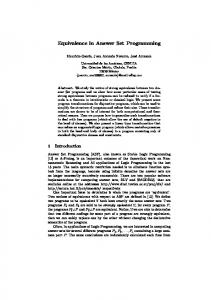
Fig. 2. Overestimate and underestimate improvement during execution In order to further confirm the above observations, we analyze in detail the behavior of the algorithms after simplifications. In particular, Figure 2 plots both the number of sound answers (line below) and the number of candidate answers (line above) over time. In particular, Figure 2(b) is devoted to the starred algorithms on an instance of MCS, whereas Figure 2(a) plots the behavior of the basic algorithms on the same instance. First, we note that A3 and A4 perform similarly and outperform A2, which timed out. Notably, A2∗ can produce the underestimate (see the bottom line in Figure 2(b)) whereas A2 can only print the overestimate (there is no underestimate line for A2 in Figure 2(a)). In general, A3 and A4 are able to improve their estimates better than A2. Note that there is a point in the plots for each improvement of estimates, and lines are very dense on MCS instances. This confirms that MCS instances have a huge number of stable models that can be rapidly computed. We observed an analogous behavior for CQA. Plots for SBB instances on Figure 2(c) and Figure 2(d) have, instead, sparse lines, confirming that stable model search is harder for this benchmark. Nevertheless, the starred algorithms can rapidly pro-

10

M. Alviano, C. Dodaro and F. Ricca 

 

 

Up to timeout %

 M

%&'

A2 A2* A3* A4* multi

A2 A2* A3* A4* mu!ti



&*,

A2 A2* A3* A4* multi

A2 A2* A3* A4* mu!ti

SS

'--

A2 A2* A3* A4* multi

A2 A2* A3* A4* mu!ti 0%

2%

0%

(a) Sound answers

%

00%

0%

2"%

"0%

#"%

$00%

(b) Candidates reduction

Fig. 3. Sound answers and candidates reduction after simplification

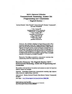
duce most of the sound answers. A deeper look at Figure 2(c) suggests that A2 is much faster than both A3 and A4 in solving this instance. In fact, it improves the overestimate faster than any other algorithm. Figure 2(e) and Figure 2(f) focus on multi and its components. In Figure 2(f), multi is faster and improves estimates better than A2∗ and A4∗ . In contrast, multi is slower than A2∗ in Figure 2(e). A possible cause is the information exchange among processes that modifies the program handled by A2∗ with constraints produced by A3∗ , which in this case results in an harder instance also for the A2∗ process. Note that multi has a non-deterministic behavior due to its parallel nature. Indeed, information exchanged may be different in different runs. More insights on the general behavior of the algorithms in the non-deterministic part of the computation can be obtained by looking at Figure 3. In particular, Figure 3(a) reports the average percentage of sound answers produced after the simplification step, while candidates reduction is shown on Figure 3(b). A3 is not shown in the figure because it performs similarly to A3∗ in this perspective. The same holds for A4 and A4∗ . We point out that all bars refer to sound answers and candidates remaining after simplifications, also for A2. As a general observation, A2 prints sound answers only at the end of the computation, while other algorithms are anytime. Consequently, A2 does not provide sound answers as soon as the other algorithms, as shown on Figure 3(a). Basically, A2 can print something in the first 10s only for easy instances, while A2∗ improves a lot in this respect. For example, A2∗ outputs around 14% of sound answers already in the first 10s of computation in MCS, while A2 produces no output. Nonetheless, A3∗ and A4∗ perform generally better than A2∗ . The difference between A3∗ and A4∗ emerges only in SBB, where finding stable models is harder. In particular, by looking at Figure 3(a), A4∗ produces more sound answers than A3∗ , whereas A3∗ is more effective in reducing the number of candidates on Figure 3(b). Note that A4∗ may change the candidate to test at each restart, and in our implementation it selects the one with the largest value of activity (which very roughly means the one that was involved more often in conflicts). On the other hand, A3∗ insists on the same candidate until the end of a stable model search. As a consequence, A4∗ has more chances to find inconsistent branches and, therefore, to improve the underestimate. On the contrary, A3∗ has more chances to find a stable model and, thus, to improve the overestimate. This suggests that A4∗ should be preferred, since it outputs sound answers more frequently, and also because, as discussed above, A4∗ is faster than A3∗ on the average (see Table 1). Concerning multi, we observe that it outperforms

Anytime Computation of Cautious Consequences in Answer Set Programming 600

600 A2 A2* A3* A4* multi

500

A2 A2* A3* A4* multi

500

400 Execution time (s)

400 Execution time (s)

11

300

300

200

200

100

100

0

0 0

10

20

30

40 50 Number of instances

60

70

80

90

0

(a) 25% of sound answers

10

20

30 40 Number of instances

50

60

70

(b) 100% of sound answers

Fig. 4. Time performance of algorithms for computing underestimates the alternatives on CQA and SBB, while it is less effective in printing sound answers on the average for SBB instances. This is due to the presence of an outlier in this benchmark that spoils the average. That outlier can be explained by the already discussed non-deterministic behavior of multi. Analogous considerations can be done for the reduction of candidates on Figure 3(b). Another perspective on the behavior of the various algorithms can be obtained by looking at Figure 4. Here are reported, for each benchmark, two variants of the classical cactus plot. Recall that, in a cactus plot, the x-axis reports the number of instances that are solved within the time reported on the y-axis. Here we consider variants where on the x-axis is the number of instances for which an algorithm printed 25% (resp. 100%) of sound answers within the time reported on the y-axis. We point out that anytime solvers can print 100% of sound answers before the timeout, even if termination is not reached within the allotted time. Figure 4 confirms that A2 is slower than anytime algorithms in printing sound answers. It is interesting to note that the anytime A2∗ improves sensibly A2 in all benchmarks, especially at the beginning of the computation. We also observe that A4∗ is slightly preferable to A3∗ , and multi is the fastest solution. Note that the differences are more evident in the plots on the left that focus on the first 25% of sound answers. Finally, we confirm that A2∗ is the fastest single-process implementation in SBB. Nonetheless, A3∗ and A4∗ print more sound answers also in non-terminating instances. To sum up, anytime algorithms are convenient in practice because they determine several sound answers already in the first steps of computation. In particular, the starred variants are preferable (A4∗ leading the group) because they provide sound answers as soon as possible and are thus effective also in non-terminating instances. Finally, the parallel system combining A4∗ with A2∗ is the best variant overall.

5 Related Work The computation of cautious consequences in ASP is a feature available in two solvers, namely DLV (Maratea et al. 2008) and clasp (Gebser et al. 2012a). The algorithm implemented by DLV is enumeration of models, while clasp implements overestimate reduction. Our implementation differs from these solvers especially with respect to the output produced during the computation of cautious consequences. In fact, DLV does not print any form of estimation during the computation, and clasp only prints overestimates. Our implementation, instead, is anytime and thus prints both underestimates and overestimates during the computation. Underestimates provide sound answers also when termination is not affordable in reasonable time, and are thus of practi-

12

M. Alviano, C. Dodaro and F. Ricca

cal importance for hard problems. It is interesting to observe that among the strategies supported by our implementation there is A2∗ , an anytime variant of the algorithm used by clasp that performed very well on two of our three benchmarks. We also note that DLV and clasp feature brave reasoning, which is not currently supported by our implementation. Clasp, being a parallel ASP solver (Gebser et al. 2012b), also supports the parallel computation of cautious consequences by means of the overestimate reduction algorithm. Our proposal is different, as it is based on the combination of two different algorithms, namely iterative partial coherence testing and overestimate reduction, for reducing both estimates at the same time. However, we observe that our parallel implementation is a proof-of-concept prototype obtained by combining two instances of WASP (properly modified to share short learned constraints and answer estimates) controlled by a Python script. It is devised to show the benefits of combining two different algorithms, while a more efficient implementation is subject of future work. The computation of cautious consequences of a ground program is related to the problem of backbone computations of propositional formulas (Marques-Silva et al. 2010; Slaney and Walsh 2001). In fact, the backbone of a propositional formula ϕ is the set of literals that are true in all models of ϕ . Several algorithms for computing backbones of propositional formulas are based on variants of the iterative consistency testing algorithm (Marques-Silva et al. 2010; Janota et al. 2014), which essentially corresponds to the iterative coherence testing algorithm analyzed in this paper. Backbone search algorithms usually feature additional techniques for removing candidates to be tested, such as implicant reduction and core-based chunking (Ravi and Somenzi 2004). Most of the implicant reduction techniques are not applicable to normal ASP programs because of the intrinsic minimality of stable models. For example, backbone search algorithms can reduce their overestimate by removing all unassigned variables when a (partial) model is found; in our setting, ASP solvers always terminate with a complete assignment. Core-based chunking, instead, requires a portfolio of algorithms (Janota et al. 2014) in order to be effective, which is beyond the scope of this paper. Note that all considered algorithms work on ground programs. Combinations with query optimization techniques such as magic sets (Greco 2003; Alviano and Faber 2011) are possible but not the focus of the paper.

6 Conclusion Several algorithms for computing cautious consequences of ASP programs were analyzed in this paper. At the time of this writing, ASP solvers do not implement anytime algorithms, which means that computation must terminate in order to obtain some cautious consequences. On the other hand, the computation of cautious consequences is similar to the computation of backbones of propositional theories, for which anytime algorithms do exist. We adapted one of these algorithms to cautious reasoning, showing that underestimates can be effectively obtained in reasonable time also for hard instances. Moreover, we introduced a general strategy to obtain anytime variants of existing algorithms such as those implemented by DLV and clasp. All algorithms as well as a proof-of-concept parallel implementation were implemented in the solver WASP. Our empirical evaluation highlights that sound answers are computable within the first seconds of computation in many cases. Moreover, the performance of the parallel system is encouraging and leaves space for future work on this subject. Acknowledgements. This research has been partly supported by Regione Calabria under the

Anytime Computation of Cautious Consequences in Answer Set Programming

13

EU Social Fund and project PIA KnowRex POR FESR 2007- 2013, and the Italian Ministry of University and Research under PON project “Ba2Know S.I.-LAB” n. PON03PE 0001. References A LVIANO , M., D ODARO , C., FABER , W., L EONE , N., AND R ICCA , F. 2013. WASP: A native ASP solver based on constraint learning. In LPNMR, P. Cabalar and T. C. Son, Eds. LNCS, vol. 8148. Springer, 54–66. A LVIANO , M. AND FABER , W. 2011. Dynamic magic sets and super-coherent answer set programs. AI Communications. IOS Press 24, 2, 125–145. A LVIANO , M., FABER , W., L EONE , N., P ERRI , S., P FEIFER , G., AND T ERRACINA , G. 2011. The disjunctive datalog system DLV. In Datalog 2.0, G. Gottlob, Ed. Vol. 6702. Springer Berlin/Heidelberg, 282–301. A RENAS , M., B ERTOSSI , L. E., AND C HOMICKI , J. 2003. Answer sets for consistent query answering in inconsistent databases. Theory and Practice of Logic Programming 3, 4-5, 393–424. BARAL , C. 2003. Knowledge Representation, Reasoning and Declarative Problem Solving. Cambridge University Press. B REWKA , G. AND E ITER , T. 2007. Equilibria in heterogeneous nonmonotonic multi-context systems. In AAAI. AAAI Press, 385–390. C ALIMERI , F., I ANNI , G., AND R ICCA , F. 2014. The third open answer set programming competition. Theory and Practice of Logic Programming 14, 1, 117–135. DAVIS , M., L OGEMANN , G., AND L OVELAND , D. 1962. A machine program for theorem proving. Commun. ACM 5, 394–397. E E´ N , N. AND B IERE , A. 2005. Effective preprocessing in SAT through variable and clause elimination. In SAT. LNCS, vol. 3569. Springer, 61–75. ¨ E E´ N , N. AND S ORENSSON , N. 2003a. An extensible SAT-solver. In SAT, E. Giunchiglia and A. Tacchella, Eds. LNCS, vol. 2919. Springer, 502–518. ¨ E E´ N , N. AND S ORENSSON , N. 2003b. Temporal induction by incremental sat solving. Electr. Notes Theor. Comput. Sci. 89, 4, 543–560. E ITER , T. 2005. Data integration and answer set programming. In LPNMR, C. Baral, G. Greco, N. Leone, and G. Terracina, Eds. LNCS, vol. 3662. Springer, 13–25. E ITER , T., I ANNI , G., L UKASIEWICZ , T., S CHINDLAUER , R., AND T OMPITS , H. 2008. Combining answer set programming with description logics for the semantic web. Artif. Intell. 172, 12-13, 1495– 1539. G ASCHNIG , J. 1979. Performance measurement and analysis of certain search algorithms. Ph.D. thesis, Carnegie Mellon University, Pittsburgh, PA, USA. Technical Report CMU-CS-79-124. ¨ G EBSER , M., K AMINSKI , R., K ONIG , A., AND S CHAUB , T. 2011. Advances in gringo series 3. In LPNMR, J. P. Delgrande and W. Faber, Eds. LNCS, vol. 6645. Springer, 345–351. G EBSER , M., K AUFMANN , B., AND S CHAUB , T. 2012a. Conflict-driven answer set solving: From theory to practice. Artif. Intell. 187, 52–89. G EBSER , M., K AUFMANN , B., AND S CHAUB , T. 2012b. Multi-threaded ASP solving with clasp. Theory and Practice of Logic Programming 12, 4-5, 525–545. G ELFOND , M. AND K AHL , Y. 2014. Knowledge Representation, Reasoning, and the Design of Intelligent Agents: The Answer-Set Programming Approach. Cambridge University Press. G ELFOND , M. AND L IFSCHITZ , V. 1991. Classical negation in logic programs and disjunctive databases. New Generation Computing 9, 365–385. G OMES , C. P., S ELMAN , B., AND K AUTZ , H. A. 1998. Boosting combinatorial search through randomization. In Proceedings of AAAI/IAAI 1998. AAAI Press, 431–437. G RECO , S. 2003. Binding propagation techniques for the optimization of bound disjunctive queries. IEEE Transactions on Knowledge and Data Engineering 15, 2 (March/April), 368–385.

14

M. Alviano, C. Dodaro and F. Ricca

JANOTA , M., LYNCE , I., AND M ARQUES -S ILVA , J. 2014. Algorithms for computing backbones of propositional formulae. AI Commun.. To appear. ¨ J ARVISALO , M., B ERRE , D. L., ROUSSEL , O., AND S IMON , L. 2012. The international SAT solver competitions. AI Magazine 33, 1. KOLAITIS , P. G., P EMA , E., AND TAN , W.-C. 2013. Efficient querying of inconsistent databases with binary integer programming. PVLDB 6, 6, 397–408. L EONE , N., P FEIFER , G., FABER , W., E ITER , T., G OTTLOB , G., P ERRI , S., AND S CARCELLO , F. 2006. The DLV system for knowledge representation and reasoning. ACM Transactions on Computational Logic 7, 3 (July), 499–562. L IERLER , Y. AND M ARATEA , M. 2004. Cmodels-2: SAT-based answer set solver enhanced to nontight programs. In Proceedings of the 7th International Conference on Logic Programming and NonMonotonic Reasoning (LPNMR-7), V. Lifschitz and I. Niemel¨a, Eds. LNAI, vol. 2923. Springer, 346– 350. L IFSCHITZ , V. 2002. Answer set programming and plan generation. Artificial Intelligence 138, 39–54. L IFSCHITZ , V. AND T URNER , H. 1994. Splitting a logic program. In Proceedings of the 11th International Conference on Logic Programming (ICLP’94), P. Van Hentenryck, Ed. MIT Press, Santa Margherita Ligure, Italy, 23–37. L UBY, M., S INCLAIR , A., AND Z UCKERMAN , D. 1993. Optimal speedup of Las Vegas algorithms. Inf. Process. Lett. 47, 173–180. M ANNA , M., R ICCA , F., AND T ERRACINA , G. 2013. Consistent query answering via ASP from different perspectives: Theory and practice. Theory and Practice of Logic Programming 13, 2, 227–252. M ARATEA , M., R ICCA , F., FABER , W., AND L EONE , N. 2008. Look-back techniques and heuristics in dlv: Implementation, evaluation, and comparison to qbf solvers. J. Algorithms 63, 1-3, 70–89. ´ M AREK , V. W. AND T RUSZCZY NSKI , M. 1999. Stable models and an alternative logic programming paradigm. In The Logic Programming Paradigm – A 25-Year Perspective, K. R. Apt, V. W. Marek, M. Truszczy´nski, and D. S. Warren, Eds. Springer Verlag, 375–398. M ARQUES -S ILVA , J., JANOTA , M., AND LYNCE , I. 2010. On computing backbones of propositional theories. In ECAI, H. Coelho, R. Studer, and M. Wooldridge, Eds. Frontiers in Artificial Intelligence and Applications, vol. 215. IOS Press, 15–20. N IEMEL A¨ , I. 1999. Logic programming with stable model semantics as constraint programming paradigm. Annals of Mathematics and Artificial Intelligence 25, 3–4, 241–273. R AVI , K. AND S OMENZI , F. 2004. Minimal assignments for bounded model checking. In TACAS, K. Jensen and A. Podelski, Eds. LNCS, vol. 2988. Springer, 31–45. S LANEY, J. K. AND WALSH , T. 2001. Backbones in optimization and approximation. In IJCAI, B. Nebel, Ed. Morgan Kaufmann, 254–259. Z HANG , L., M ADIGAN , C. F., M OSKEWICZ , M. W., AND M ALIK , S. 2001. Efficient conflict driven learning in boolean satisfiability solver. In Proceedings of the International Conference on ComputerAided Design (ICCAD 2001). 279–285.

Appendix A Proof of Theorem 1 The proof is split into several lemmas using Pi , Li ,Ui , Oi , Ii to denote the content of variables P, L,U, O, I at step i of computation (i ≥ 0). More in detail, in Lemma 1 we will first show that underestimates form an increasing sequence and, on the contrary, overestimates form a decreasing sequence. Then, in Lemma 2 we will prove properties of stable models of programs Pi ∪Li (i ≥ 0). Correctness of estimates will be shown in Lemmas 3–4, and termination of the algorithms in Lemma 5. Finally, in Lemma 6 we will extend the proof to variants using ComputeStableModel∗. Lemma 1 Ui ⊆ Ui+1 and Oi+1 ⊆ Oi ⊆ Q for each i ≥ 0.

Anytime Computation of Cautious Consequences in Answer Set Programming

15

Proof Variable U is initially empty. EnumerationOfModels and OverestimateReduction reassign U only once. IterativeCoherenceTesting and UnderestimateReduction always enlarge the set stored in U by means of set union (line 4). Concerning variable O, it is initially equal to Q and restricted at each reassignment by means of set intersection (line 7 for OverestimateReduction; line 6 for the other procedures). Lemma 2 SM(Pi+1 ∪ Li+1 ) ⊆ SM(Pi ∪ Li ) for each i ≥ 0. For IterativeCoherenceTesting and IterativePartialCoherenceTesting we also have SM(Pi+1 ∪ Li+1 ) = SM(Pi ∪ Li ) for each i ≥ 0. Proof Variable P is reassigned only by EnumerationOfModels and OverestimateReduction, where constraints are added to the previous program. Constraints can only remove stable models (as a consequence of the Splitting Set Theorem by Lifschitz and Turner 1994). On the other hand, learned constraints stored in variable L are implicit in the program stored by variable P, and thus cannot change its semantics. Lemma 3 Oi ⊇ Q ∩CC(P) for each i ≥ 0. Proof The base case is true because O0 = Q. Assume the claim is true for some i ≥ 0 and consider Oi+1 = Oi ∩ Ii+1 , where Ii+1 ∈ SM(Pi ∪ Li ). By i applications of Lemma 2, we obtain Ii+1 ∈ SM(P0 ∪ L0 ), i.e., Ii+1 ∈ SM(P). We can thus conclude a ∈ Oi \ Oi+1 implies a ∈ / CC(P), and we are done. Lemma 4 Ui ⊆ Q ∩CC(P) for each i ≥ 0. Proof The base case is true because U0 = 0. / Assume the claim is true for some i ≥ 0 and consider Ui+1 . If Ui+1 = Ui then the claim is true. Otherwise, we distinguish two cases. For IterativeCoherenceTesting and IterativePartialCoherenceTesting,Ui+1 = Ui ∪{a} for some a ∈ Oi \ Ui . Moreover, there is no M ∈ SM(Pi ∪ Li ) such that a ∈ / M because Ii+1 = ⊥. From Lemma 2, we can conclude that there is no M ∈ SM(P) such that a ∈ / M, i.e., a ∈ CC(P). Since a ∈ Oi \ Ui , we have a ∈ Oi and thus a ∈ Q by Lemma 1. Therefore, a ∈ Q ∩CC(P) and we are done. For EnumerationOfModels and OverestimateReduction, Ui+1 = Oi and the algorithm terminates. Exactly i + 1 constraints were added to P, one for each stable model of P found, i.e., I1 , . . . , Ii . Moreover, Ii+1 = ⊥ holds. Assume by contradiction that there is a ∈ Oi \CC(P). Hence, there is M ∈ SM(P) such that a ∈ / M. Moreover, a ∈ I j ( j = 1, . . . , i) and thus M is a model of all constraints added at line 1. Consequently, M is a stable model of Pi ∪ Li , which contradicts Ii+1 = ⊥.

16

M. Alviano, C. Dodaro and F. Ricca

Lemma 5 Algorithm 1 terminates after finitely many steps. Proof When EnumerationOfModels is used, termination is guaranteed because P has a finite number of stable models. OverestimateReduction either sets U equal to O, or reduces O, which initially is equal to Q, a finite set. IterativeCoherenceTesting either increases U, or reduces O, and thus terminates because O is finite and Ui ⊆ Oi holds for each i ≥ 0 by Lemmas 3 and 4. Termination of IterativePartialCoherenceTesting is guaranteed if restarts are properly delayed during the computation, as it must be done already for guaranteeing termination of stable model search. Lemma 6 Underestimates produced by ComputeStableModel∗ are sound. Proof Follows by the fact that L contains constraints that are implicit in the program stored by variable P.