Complex Optimization in Answer Set Programming

Under consideration for publication in Theory and Practice of Logic Programming

1

arXiv:1107.5742v1 [cs.LO] 28 Jul 2011

Complex Optimization in Answer Set Programming Martin Gebser and Roland Kaminski and Torsten Schaub∗ Institut für Informatik, Universität Potsdam submitted [TBA]; revised [TBA]; accepted [TBA]

Abstract Preference handling and optimization are indispensable means for addressing non-trivial applications in Answer Set Programming (ASP). However, their implementation becomes difficult whenever they bring about a significant increase in computational complexity. As a consequence, existing ASP systems do not offer complex optimization capacities, supporting, for instance, inclusion-based minimization or Pareto efficiency. Rather, such complex criteria are typically addressed by resorting to dedicated modeling techniques, like saturation. Unlike the ease of common ASP modeling, however, these techniques are rather involved and hardly usable by ASP laymen. We address this problem by developing a general implementation technique by means of meta-programming, thus reusing existing ASP systems to capture various forms of qualitative preferences among answer sets. In this way, complex preferences and optimization capacities become readily available for ASP applications.

1 Introduction Preferences are often an indispensable means in modeling since they allow for identifying preferred solutions among all feasible ones. Accordingly, many forms of preferences have already found their way into systems for Answer Set Programming (ASP; (Baral 2003)). For instance, smodels provides optimization statements for expressing cost functions on sets of weighted literals (Simons et al. 2002), and dlv (Leone et al. 2006) offers weak constraints for the same purpose. Further approaches (Delgrande et al. 2003; Eiter et al. 2003) allow for expressing various types of preferences among rules. Unlike this, no readily applicable implementation techniques are available for qualitative preferences among answer sets, like inclusion minimality, Pareto-based preferences as used in (Sakama and Inoue 2000; Brewka et al. 2004), or more complex combinations as proposed in (Brewka 2004). This shortcoming is due to their higher expressiveness leading to a significant increase in computational complexity, lifting decision problems (for normal logic programs) from the first to the second level of the polynomial time hierarchy (cf. (Garey and Johnson 1979)). Roughly speaking, preferences among answer sets combine an NP with a coNP problem. The first one defines feasible solutions, while the second one ensures that there are no better solutions according to the preferences at hand. For implementing such problems, Eiter and Gottlob invented in (1995) the saturation technique, using the elevated complexity of disjunctive logic programming. In stark contrast

∗ Affiliated with Simon Fraser University, Canada, and Griffith University, Australia.

2

Martin Gebser and Roland Kaminski and Torsten Schaub

to the ease of common ASP modeling (e.g., strategic companies can be “naturally” encoded (Leone et al. 2006) in disjunctive ASP), however, the saturation technique is rather involved and hardly usable by ASP laymen. For taking this burden of intricate modeling off the user, we propose a general, saturation-based implementation technique capturing various forms of qualitative preferences among answer sets. This is driven by the desire to guarantee immediate availability and thus to stay within the realm of ASP rather than to build separate (imperative) components. To this end, we take advantage of recent advances in ASP grounding technology, admitting an easy use of meta-modeling techniques. The idea is to reinterpret existing optimization statements in order to express complex preferences among answer sets. While, for instance in smodels, the meaning of #minimize is to compute answer sets incurring minimum costs, we may alternatively use it for selecting inclusion-minimal ones. In contrast to the identification of minimal models, investigated by Janhunen and Oikarinen in (2004; 2008), a major challenge lies in guaranteeing the stability property of implicit counterexamples, which must be more preferred answer sets rather than (arbitrary) models. For this purpose, we develop a refined meta-program qualifying answer sets as viable counterexamples. Unlike the approach of Eiter and Polleres (2006), our encoding avoids “guessing” a level mapping to describe the formation of a counterexample, but directly denies models for which there is no such construction. Notably, our meta-programs apply to (reified) extended logic programs (Simons et al. 2002), possibly including choice rules and #sum constraints, and we are unaware of any existing meta-encoding of their answer sets, neither as candidates nor as counterexamples refuting optimality.

2 Background We consider extended logic programs (Simons et al. 2002) allowing for (proper) disjunctions in heads of rules (Gelfond and Lifschitz 1991). A rule r is of the following form: H ← B1 , . . . , Bm , ∼Bm+1 , . . . , ∼Bn . By head (r) = H and body(r) = {B1 , . . . , Bm , ∼Bm+1 , . . . , ∼Bn }, we denote the head and the body of r, respectively, where “∼” stands for default negation. The head H is a disjunction a1 ∨ · · · ∨ ak over atoms a1 , . . . , ak , belonging to some alphabet A, or a #sum constraint L #sum[ℓ1 = w1 , . . . , ℓk = wk ] U . In the latter, ℓi = ai or ℓi = ∼ai is a literal and wi a non-negative integer weight for ai ∈ A and 1 ≤ i ≤ k; L and U are integers providing a lower and an upper bound. Either or both of L and U can be omitted, in which case they are identified with the (trivial) bounds 0 and ∞, respectively. A rule r such that head (r) = ⊥ (H is the empty disjunction) is an integrity constraint. Each body component Bi is either an atom or a #sum constraint for 1 ≤ i ≤ n. If body (r) = ∅, r is called a fact, and we skip “←” when writing facts below. For a set {B1 , . . . , Bm , ∼Bm+1 , . . . , ∼Bn }, a disjunction a1 ∨ · · · ∨ ak , and a #sum constraint L #sum[ℓ1 = w1 , . . . , ℓk = wk ] U , we let {B1 , . . . , Bm , ∼Bm+1 , . . . , ∼Bn }+ = {B1 , . . . , Bm }, (a1 ∨ · · · ∨ ak )+ = {a1 , . . . , ak }, and (L #sum[ℓ1 = w1 , . . . , ℓk = wk ] U )+ = [ℓi = wi | 1 ≤ i ≤ k, ℓi ∈ A]. Note that the elements of a #sum constraint form a multiset, possibly containing duplicates. For some S = {a1 , . . . , ak } or S = [a1 = w1 , . . . , ak = wk ], we define atom(S) = {a1 , . . . , ak }.

Complex Optimization in Answer Set Programming

3

A (Herbrand) interpretation is represented by the set X ⊆ A of its entailed atoms. The satisfaction relation “|=” on rules r is inductively defined as follows: • • • • •

X X X X X

|= ∼B if X 6|= B, |= (a1 ∨ · · · ∨ ak ) if {a1 , . . . , ak } ∩ X 6= ∅, P |= (L #sum[ℓ1 = w1 , . . . , ℓk = wk ] U ) if L ≤ 1≤i≤k,X|=ℓi wi ≤ U , |= body (r) if X |= ℓ for all ℓ ∈ body(r), and |= r if X |= head (r) or X 6|= body(r).

A logic program Π is a set of rules r, and X is a model of Π if X |= r for every r ∈ Π. The reduct of the head H of a rule r wrt X is H X = {a1 ∨ · · · ∨ ak } if H = a1 ∨ · · · ∨ ak , and H X = atom(H + ) ∩ X if H = L #sum[ℓ1 = w1 , . . . , ℓk = wk ] U . Furthermore, the reduct of some (positive) bodyelement B ∈ body (r)+ is B X = B if B ∈ A, and B X = P + L − 1≤i≤k,ℓi =∼ai ,ai ∈X / wi #sum B if B = L #sum[ℓ1 = w1 , . . . , ℓk = wk ] U . The reduct of Π wrt X is the following logic program: X ΠX = H ← B1X , . . . , Bm | r ∈ Π, X |= body(r), H ∈ head (r)X , body(r)+ = {B1 , . . . , Bm } . That is, for all rules r ∈ Π whose bodies are satisfied wrt X, the reduct is obtained by replacing #sum constraints in heads with individual atoms belonging to X and by eliminating negative components in bodies, where lower bounds of residual #sum constraints (with trivial upper bounds) are reduced accordingly. Finally, X is an answer set of Π if X is a model of Π such that no proper subset of X is a model of ΠX . In view of the latter condition, note that an answer set is a minimal model of its own reduct. The definition of answer sets provided above applies to logic programs containing extended constructs (#sum constraints) under “choice semantics” (Simons et al. 2002), while additionally allowing for disjunctions under minimal-model semantics (wrt a reduct). We use these features to embed extended constructs of an object program into a disjunctive meta-program, so that their combination yields optimal answer sets of the object program. To this end, we reinterpret #minimize statements of the following form: #minimize[ℓ1 = w1 @J1 , . . . , ℓk = wk @Jk ].

(1)

Like with #sum constraints, every ℓi is a literal and every wi an integer weight for 1 ≤ i ≤ k, while Ji additionally provides an integer priority level.1 Priorities allow for representing a sequence of lexicographically ordered #minimize objectives, where greater levels are more significant than smaller ones. By default, a #minimize statement distinguishes optimal answer sets of a program Π in the following way. For any X ⊆ A and integer J, let ΣX J denote the sum of weights w over all occurrences of weighted literals ℓ = w@J in (1) such that X |= ℓ. An answer set X of Π is dominated if there is an answer Y X ′ set Y of Π such that ΣYJ < ΣX J and ΣJ ′ = ΣJ ′ for all J > J, and optimal otherwise. In the following, we assume that every logic program is accompanied with one (possibly 1

Explicit priority levels are supported in recent versions of the grounder gringo (Gebser et al.). This avoids a dependency of priorities on input order, which is considered by lparse (Syrjänen) if several #minimize statements are provided. Priority levels are also supported by dlv (Leone et al. 2006) in weak constraints. Furthermore, we admit negative weights in #minimize statements, where they cannot raise semantic problems (cf. (Ferraris 2005)) going along with the rewriting of #sum constraints suggested in (Simons et al. 2002).

4


empty) #minimize statement of the form (1). Instead of the default semantics, we consider Pareto efficiency wrt priority levels J, weights w, and several distinct optimization criteria. In view of this, we use levels for inducing a lexicographic order, while weights are used for grouping literals (rather than summation). Pareto improvement then builds upon a two-dimensional structure of orderings among answer sets, induced by J and w. In turn, each such pairing is associated with some of the following orderings. By Y ≤w J X, we denote that the cardinality of the multiset of occurrences of ℓ = w@J in (1) such that Y |= ℓ is not greater than the one of the corresponding multiset for X |= ℓ. Furthermore, we write Y ⊆w J X if, for any weighted literal ℓ = w@J occurring in (1), Y |= ℓ implies X |= ℓ. As detailed in the extended version of this paper (Gebser et al. 2011), we additionally consider the approach of (Sakama and Inoue 2000) and denote by Y w J X that Y is preferable to X according to a (given) preference relation among literals ℓ such that ℓ = w@J occurs in (1). Given a logic program Π and a collection M of relations of the form ⋄w J for priority levels J, weights w, and ⋄ ∈ {≤, ⊆, }, an answer set Y of Π dominates an answer set X of Π wrt M if there are a priority level J and a weight w such w w′ w′ that X ⋄w J Y does not hold for ⋄J ∈ M , while Y ⋄J ′ X holds for all ⋄J ′ ∈ M where J ′ ≥ J. In turn, an answer set X of Π is optimal wrt M if there is no answer set Y of Π that dominates X wrt M . As an example, consider the following program, referred to by Π0 : 1 {p, t}

← 1 {r, s, ∼t} 2.

(2)

{q, r} 1 ← 1 {p, t}.

(3)

← ∼q, ∼r.

(4)

s

This program has five answer sets, viz. {p, q}, {p, r}, {p, s}, {p, s, t}, and {s, t}. (Sets {a1 , . . . , ak } in (2) and (3) are used as shorthands for #sum[a1 = 1, . . . , ak = 1].) In addition, let Π1 denote the union of Π0 with the following #minimize statement: #minimize[p = 1@1, q = 1@1, r = 1@1, s = 1@1].

(5)

This statement specifies that all atoms of Π0 except for t are subject to minimization. Passing Π1 to gringo and an answer set solver like smodels yields the single ≤11 -minimal answer set {s, t}. Note, however, that Π0 has three ⊆11 -minimal answer sets, namely {p, q}, {p, r}, and {s, t}. They cannot be computed directly from Π1 via any available ASP system. We implement the complex optimization criteria described above by meta-interpretation in disjunctive ASP. For transparency, we provide meta-programs as true ASP code in the first-order input language of gringo (Gebser et al.), including not and | as tokens for ∼ and ∨, respectively, as well as {a1 ,. . . ,ak } as shorthand for #sum[a1 =1,. . . ,ak =1]. Further constructs are informally introduced by need in the remainder of this paper. Note that our (disjunctive) meta-programs apply to an extended object program that does not include proper disjunctions (over more than one atom). Unless stated otherwise, we below use the term extended program to refer to a logic program without proper disjunctions. 3 Basic Meta-Modeling For reinterpreting #minimize statements by means of ASP, we take advantage of recent advances in ASP grounding, admitting an easy use of meta-modeling techniques. To be

Complex Optimization in Answer Set Programming 1 2 3 4

rule(pos(sum(1,0,2)),pos(conjunction(0))). % 1 { p, t } :- 1 { r, s, not t } 2. wlist(0,0,pos(atom(p)),1). wlist(0,1,pos(atom(t)),1). set(0,pos(sum(1,1,2))). wlist(1,0,pos(atom(r)),1). wlist(1,1,pos(atom(s)),1). wlist(1,2,neg(atom(t)),1).

6 7 8

rule(pos(sum(0,2,1)),pos(conjunction(1))). % { q, r } 1 :- 1 { p, t }. wlist(2,0,pos(atom(q)),1). wlist(2,1,pos(atom(r)),1). set(1,pos(sum(1,0,2))).

10 11

rule(pos(atom(s)),pos(conjunction(2))). set(2,neg(atom(q))). set(2,neg(atom(r))).

13 14 15

scc(0,pos(atom(p))). scc(0,pos(atom(r))). scc(0,pos(atom(t))). scc(0,pos(conjunction(0))). scc(0,pos(sum(1,1,2))). scc(0,pos(conjunction(1))). scc(0,pos(sum(1,0,2))).

17 18 19

minimize(1,3). % #minimize [ p = 1 @ 1, q = 1 @ 1, r = 1 @ 1, s = 1 @ 1 ]. wlist(3,0,pos(atom(p)),1). wlist(3,1,pos(atom(q)),1). wlist(3,2,pos(atom(r)),1). wlist(3,3,pos(atom(s)),1).

5

% s :- not q, not r.

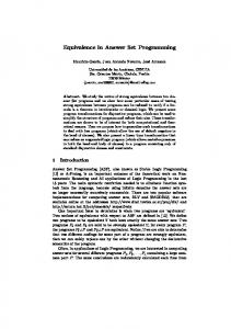
Listing 1. Facts describing a reified extended logic program.

precise, we rely upon the unrestricted usage of function symbols and program reification as provided by gringo (Gebser et al.). The latter allows for turning an input program along with a #minimize statement into facts representing the structure of their ground instantiation. For illustrating the format output by gringo, consider the facts in Line 1–15 of Listing 1, obtained by calling gringo with option --reify on program Π0 . Let us detail the representation of the rule in (2) inducing the facts in Line 1–4. The predicate rule/2 is used to link the rule head and body. By convention, both are positive rule elements, as indicated via the functor pos/1. Furthermore, the term sum(1,0,2) tells us that the head is a #sum constraint with lower bound 1 and (trivial) upper bound 2 over a list labeled 0 of weighted literals. In fact, the included literals are provided via the facts over wlist/4 given in Line 2, whose first arguments are 0. While the second arguments, 0 and 1, are simply indexes (enabling the representation of duplicates in multisets), the third ones provide literals, p and t, each having the (default) weight 1, as given in the fourth arguments. Again by convention, the body of each rule is a conjunction, where the term conjunction(0) in Line 1 refers to the set labeled 0. Its single element, a positive #sum constraint with lower bound 1 and upper bound 2 over a list labeled 1, is provided by the fact in Line 3. The corresponding weighted literals are described by the facts in Line 4; observe that the negative literal not t is represented in terms of the functor neg/1, applied to atom(t). The rules in (3) and (4) are represented analogously in Line 6–8 and 10–11, respectively. It is still interesting to note that recurrences of lists of weighted literals (and sets) can reuse labels introduced before, as done in Line 8 by referring to 0. In fact, gringo identifies repetitions of structural entities and reuses labels. In addition to the rules of Π0 , the elements of non-trivial strongly connected components of its positive dependency graph (cf. (6) below) are provided in Line 13–15. Albeit their usage is explained in the next section, note already that the members of the only such component, labeled 0, include atoms as well as (positive) body elements, i.e., conjunctions and #sum constraints, connecting the component. Indeed, the existence of facts over scc/2 tells us that Π0 is not tight (cf. (Fages 1994)).

6


1

% extract rule elements

3 4 5

litb(B) :- rule(_,B). litb(E) :- litb(pos(conjunction(S))), set(S,E). litb(E) :- eleb(sum(_,S,_)), wlist(S,_,E,_).

7 8

eleb(P) :- litb(pos(P)). eleb(N) :- litb(neg(N)).

10 11 12 13

elem(E) elem(E) elem(P) elem(N)

15

% generate answer set from reified rules

17 18 19 20 21 22

hold(conjunction(S)) :- eleb(conjunction(S)), hold(P) : set(S,pos(P)), not hold(N) : set(S,neg(N)). hold(sum(L,S,U)) :- eleb(sum(L,S,U)), L #sum [ hold(P) = W : wlist(S,Q,pos(P),W), not hold(N) = W : wlist(S,Q,neg(N),W) ] U.

24 25 26 27 28

hold(atom(A)) :- rule(pos(atom(A)), pos(B)), hold(B). L #sum [ hold(P) = W : wlist(S,Q,pos(P),W), not hold(N) = W : wlist(S,Q,neg(N),W) ] U :- rule(pos(sum(L,S,U)),pos(B)), hold(B). :- rule(pos(false), pos(B)), hold(B).

30

% project output to atoms of answer set

32

#hide. #show hold(atom(A)).

::::-

eleb(E). rule(pos(E),_). rule(pos(sum(_,S,_)),_), wlist(S,_,pos(P),_). rule(pos(sum(_,S,_)),_), wlist(S,_,neg(N),_).

Listing 2. Basic meta-program (meta.lp) for reified extended logic programs. Now, we may compute all five answer sets of Π0 (given in p0.lp) by combining the facts in Line 1–15 of Listing 1 with the basic meta-program in Listing 2 (meta.lp):2 gringo --reify p0.lp | gringo meta.lp - | clasp 0 Each answer set of the meta-program applied to a reified program corresponds to an answer set of the reified program. More precisely, a set X of atoms is an answer set of the reified program iff the meta-program yields an answer set Y such that X = {a | hold(atom(a)) ∈ Y }, e.g., hold(atom(q)) stands for q. As indicated in the comments (preceded by %), our meta-program consists of three parts. Among the rule elements extracted in Line 3–13, only those occurring within bodies, identified via eleb/1, are relevant to the generation of answer sets specified in Line 17–28. (Additional head elements, given by elem/1, are of interest in the next section.) In fact, answer set generation follows the structure of reified programs, identifying conjunctions and #sum constraints that hold3 to further derive atoms occurring in rule heads, either singular or within #sum constraints (cf. Line 24–27). Line 28 deals with integrity constraints represented via the constant false in heads of reified rules. The last part in Line 32 restricts the output of the meta-program’s answer sets to the representations of original input atoms. Finally, note that meta.lp does not inspect facts representing a reified #minimize statement, such as the ones in Line 17–19 of Listing 1 stemming from the statement in (5).

2 3

Following Unix customs, the minus symbol “-” stands for the output of “gringo --reify p0.lp.” The “:” connective expands to the list of all instances of its left-hand side such that corresponding instances of literals on the right-hand side hold (cf. (Syrjänen) and (Gebser et al.)).

Complex Optimization in Answer Set Programming

7

Such facts over minimize/2 provide a priority level as the first argument and the label of a list of weighted literals, like the ones referred to from within terms of functor sum/3, as the second argument. Rather than simply mirroring the standard meaning of #minimize statements (by encoding them analogously to rules; cf. Line 17–28 of Listing 2), we support flexible customizations. In fact, the next section presents our meta-programs implementing preference relations and Pareto efficiency, as described in the background. 4 Advanced Meta-Modeling Given the reification of extended logic programs and the encoding of their answer sets in meta.lp, our approach to complex optimization is based on the idea that an answer set generated via meta.lp is optimal (and thus acceptable) only if it is not dominated by any other answer set. For implementing our approach, we exploit the capabilities of disjunctive ASP to compactly represent the space of all potential counterexamples, viz. answer sets dominating a candidate answer set at hand. To this end, we encode the subtasks of 1. guessing an answer set as a potential counterexample and 2. verifying that the counterexample dominates a candidate answer set. A candidate answer set passes both phases if it turns out to be infeasible to guess a counterexample that dominates it. For expressing the non-existence of counterexamples, we make use of an error-indicating atom bot and saturation (Eiter and Gottlob 1995), deriving all atoms representing the space of counterexamples from bot. Since the semantics of disjunctive ASP is based on minimization, saturation makes sure that bot is derived only if it is inevitable, i.e., if it is impossible to construct a counterexample. However, via an integrity constraint, we can stipulate bot (and thus the non-existence of counterexamples) to hold, yet without providing any derivation of bot. In view of such a constraint and saturation, a successful candidate answer set is accompanied by all atoms representing counterexamples. Given that the reduct drops negative literals, the necessity that all atoms representing counterexamples are true implies that we cannot use their default negation in any meaningful way. Hence, we below encode potential counterexamples, i.e., answer sets of extended programs, and (non-)dominance of a candidate answer set in disjunctive ASP without taking advantage of default negation (used in meta.lp). For encoding the first subtask of guessing a counterexample, we rely on a characterization of answer sets in terms of an immediate consequence operator T (cf. (Lloyd 1987)), defined as follows for a logic program Π and a set X ⊆ A of atoms: T Π (X) = {head (r) | r ∈ Π, X |= body (r)}. Furthermore, an iterative version of T can be defined in the following way: T Π0 (X) = X and T Πi+1 (X) = T Πi (X) ∪ T Π (T Πi (X)). In the context of an extended program Π, possibly including choice rules, default negation, and upper bounds of weight constraints, we are interested in the least fixpoint of T applied wrt the reduct ΠX . Since a fixpoint is reached in at most |atom(Π)| applications of T , where atom(Π) ⊆ A |atom(Π)| denotes the set of atoms occurring in Π, the least fixpoint is given by T ΠX (∅). As pointed out in (Liu and You 2010), a model X of an extended program Π is an answer |atom(Π)| set of Π iff T ΠX (∅) = X. Furthermore, Liu and You (2010) show that X violates the loop formula of some atom or loop if X is a model, but not an answer set of Π. This property motivates a “localization” of T on the basis of (circular) positive dependencies.

8


The (positive) dependency graph of an extended program Π is given by the following pair of nodes and directed edges: atom(Π), {(a, b) | r ∈ Π, a ∈ atom(head (r)+ ), B ∈ body(r)+ , b ∈ atom(B + )} . (6) A strongly connected component (SCC) is a maximal subgraph of the dependency graph of Π such that all nodes are pairwisely connected via paths. An SCC is trivial if it does not contain any edge, and non-trivial otherwise. Note that the SCCs of the dependency graph of Π induce a partition of atom(Π) such that every atom and every loop of Π is contained in some part. Hence, we can make use of the partition to apply T separately to each part. Proposition 1 Let Π be an extended logic program, C1 , . . . , Ck be the sets of atoms belonging to the SCCs of the dependency graph of Π, and X ⊆ atom(Π). S |C | |atom(Π)| Then, we have that T ΠX (∅) = X iff 1≤j≤k (T ΠXj (X \ Cj ) ∩ Cj ) = X. The above property is used in our encoding of answer sets (as counterexamples) in disjunctive ASP. In a nutshell, it combines the following parts: 1. guessing an interpretation, 2. deriving the error-indicating atom bot if the interpretation is not a supported model (where each true atom occurs positively in the head of some rule whose body holds), 3. deriving bot if the true atoms of some non-trivial SCC are not acyclicly derivable (checked via determining the complement of a fixpoint of T ), and 4. saturating interpretations that do not correspond to answer sets by deriving all truth assignments (for atoms) from bot. Note that the third part, checking acyclic derivability, concentrates on atoms of non-trivial SCCs, while checking support in the second part is already sufficient for trivial SCCs. The meta-program in Listing 3 implements the sketched idea. In the following, we concentrate on describing its crucial features. For evaluating support, the meta-rules in Line 3 and 4 collect atoms having a positive occurrence in the head of a rule along with the rule’s body. Note that, for atoms contained in a #sum constraint in the head, the associated bounds and weights are inessential in the context of support. On the other hand, the meta-rule in Line 6 sums the weights of all literals in a #sum constraint; this is needed to evaluate bounds in the sequel, where (non-reified) default negation and upper bounds (acting negatively) are inapplicable in view of saturation. The meta-rules in Line 10–29 generate an interpretation by guessing some truth value for each atom (Line 10) and evaluating further constructs occurring in a reified program accordingly (Line 12–29). While the special constant false (used as head of integrity constraints) holds in no interpretation (fail(false) is a fact) and the evaluation of conjunctions is straightforward, more care is required for evaluating #sum constraints. For instance, the case that a #sum constraint holds is in the meta-rule in Line 19–23 identified via sufficiently many literals that hold to achieve the lower bound L and also sufficiently many literals that do not hold to fill the gap between the upper bound U and the sum T of all weights. Note that the latter condition is encoded by the lower bound T-U, rather than taking U as an upper bound (as done in meta.lp). The complementary cases that a #sum constraint does not hold are described in the same manner in Line 24–29, where the lower

Complex Optimization in Answer Set Programming 1

% extract supports of atoms and sums of weight lists’ weights

3 4

supp(atom(A),B) :- rule(pos(atom(A)), pos(B)). supp(atom(A),B) :- rule(pos(sum(_,S,_)),pos(B)), wlist(S,_,pos(atom(A)),_).

6

sum(S,T)

8

% generate interpretation

:- elem(sum(_,S,_)), T = #sum [ wlist(S,Q,_,W) = W ].

10

true(atom(A)) | fail(atom(A)) :- elem(atom(A)).

12

fail(false).

14 15 16 17

true(conjunction(S)) :- elem(conjunction(S)), true(P) : set(S,pos(P)), fail(N) : set(S,neg(N)). fail(conjunction(S)) :- elem(conjunction(S)), set(S,pos(P)), fail(P). fail(conjunction(S)) :- elem(conjunction(S)), set(S,neg(N)), true(N).

19 20 21 22 23 24 25 26 27 28 29

true(sum(L,S,U))

31

% verify supported model properties

33 34

bot :- rule(pos(H),pos(B)), true(B), fail(H). bot :- true(atom(A)), fail(B) : supp(atom(A),B).

36

% verify acyclic derivability

38

step(C,Z)

:- scc(C,_), Z = #sum [ scc(C,pos(atom(A))) ].

40 41

sccw(A)

:- scc(C,pos(atom(A))), fail(B) : supp(atom(A),B) : not scc(C,pos(B)).

43

wait(E,D-1)

:- scc(C,pos(E)), fail(E), step(C,Z), D = 1..Z.

45 46 47

wait(atom(A),0) wait(atom(A),D)

:- scc(C,pos(atom(A))). :- scc(C,pos(atom(A))), sccw(A), step(C,Z), D = 1..Z, wait(B,D-1) : supp(atom(A),B) : scc(C,pos(B)).

49 50 51 52

wait(sum(L,S,U),D-1) :- scc(C,pos(sum(L,S,U))), sum(S,T), step(C,Z), D = 1..Z, T-L+1 #sum [ fail(P) = W : wlist(S,Q,pos(P),W) : not scc(C,pos(P)), wait(P,D-1) = W : wlist(S,Q,pos(P),W) : scc(C,pos(P)), true(N) = W : wlist(S,Q,neg(N),W) ].

54 55

wait(conjunction(S),D-1) :- scc(C,pos(conjunction(S))), set(S,pos(P)), scc(C,pos(P)), wait(P,D-1), step(C,Z), D = 1..Z.

57

bot :- scc(C,pos(atom(A))), true(atom(A)), wait(atom(A),Z), step(C,Z).

59

% saturate interpretations that are not answer sets

61 62

true(atom(A)) :- elem(atom(A)), bot. fail(atom(A)) :- elem(atom(A)), bot.

fail(sum(L,S,U))

fail(sum(L,S,U))

9

:- elem(sum(L,S,U)), sum(S,T), L #sum [ true(P) = W : wlist(S,Q,pos(P),W), fail(N) = W : wlist(S,Q,neg(N),W) ], T-U #sum [ fail(P) = W : wlist(S,Q,pos(P),W), true(N) = W : wlist(S,Q,neg(N),W) ]. :- elem(sum(L,S,U)), sum(S,T), T-L+1 #sum [ fail(P) = W : wlist(S,Q,pos(P),W), true(N) = W : wlist(S,Q,neg(N),W) ]. :- elem(sum(L,S,U)), U+1 #sum [ true(P) = W : wlist(S,Q,pos(P),W), fail(N) = W : wlist(S,Q,neg(N),W) ].

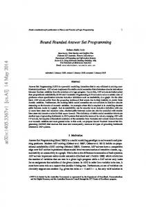
Listing 3. Disjunctive meta-program (metaD.lp) for reified extended logic programs. bound T-L+1 (or U+1) for weights of literals that do not hold (or hold) is used to indicate a violated lower (or upper) bound of the reified #sum constraint. Given an interpretation of atoms and the corresponding truth values of further constructs in an extended program, the meta-rules in Line 33 and 34 are used to derive bot if the

10


interpretation does not provide us with a supported model. To avoid such a derivation of bot, every rule of the reified program must be satisfied, and every true atom must have a positive occurrence in the head of some rule whose body holds. It remains to check the acyclic derivability of atoms belonging to non-trivial SCCs. To this end, the meta-rule in Line 38 determines the number Z of atoms in an SCC labeled C as the maximum step at which a fixpoint of T , applied locally to C, is reached. Furthermore, the meta-rule in Line 40–41 derives sccw(A) if the atom referred to by A does not have a derivation external to C. (Recall that the positive body elements of rules internally connecting an SCC, i.e., rules contributing the SCC’s edges to the dependency graph, are marked by facts over scc/2; cf. Listing 1.) The acyclic derivability of atoms indicated by sccw(A) is of particular interest in the sequel. In fact, our encoding identifies the complement of a fixpoint of T in terms of atoms A for which wait(atom(A),Z) is derived. To accomplish this, the meta-rule in Line 45 marks all atoms of C as underived at step 0. As encoded via the meta-rule in Line 46–47, an atom A stays underived at a later step D if there is no external derivation of A (sccw(A) holds) and the bodies B of all componentinternal supports of A are yet underived at step D-1 (wait(B,D-1) holds). The latter is checked via the meta-rules in Line 49–52 and 54–55, respectively. The former applies to #sum constraints and identifies cases where the weights of literals that do not hold along with the ones of yet underived atoms of C exceed T-L, so that the lower bound L is not yet established. Similarly, the underivability of a conjunction is recognized via a yet underived positive body element internal to the component C. Also note that the falsity of elements of C is propagated via the meta-rule in Line 43, so that false atoms, #sum constraints, and conjunctions do not contribute to derivations of atoms of C. As mentioned above, the complement of a fixpoint of T contains the atoms A such that wait(atom(A),Z) is eventually derived. If any such atom A is true, failure to construct an answer set is indicated by deriving bot via the meta-rule in Line 57. Finally, saturation of interpretations that do not correspond to answer sets is accomplished via the meta-rules in Line 61 and 62 of Listing 3. They make sure that bot is included in an answer set of the meta-program only if it is inevitable wrt every interpretation. When considering the encoding part in Listing 3 in isolation, it like meta.lp describes answer sets of a reified program, and bot is derived only if there is no such answer set. Our meta-programs meta.lp and metaD.lp in Listing 2 and 3 have not yet considered facts minimize(J,S) in reified programs, reflecting input #minimize statements. In fact, complex optimization is addressed by the meta-program metaO.lp, shown in Listing 4. It allows for separate optimization criteria per priority level J and weight W (in facts wlist(S,Q,E,W)). Particular criteria can be provided via the user predicate optimize(J,W,O), where the values card, incl, and pref for O refer to minimality regarding cardinality, inclusion, and preference (Sakama and Inoue 2000), respectively, among the involved literals E. Such criteria are reflected via instances of cxopt(J,W,O), derived via the rules in Line 7 and 8–9, where card is taken by default if no criterion is provided by the user. At each priority level J, Pareto improvement of a counterexample (constructed via the rules in metaD.lp) over all weights W and criteria O such that cxopt(J,W,O) holds is used for deciding whether a candidate answer set (constructed via the rules in meta.lp) is optimal. To this end, similarity at a priority level J is indicated by deriving equal(J) from equal(J,W,O) over all instances of cxopt(J,W,O) via

Complex Optimization in Answer Set Programming 1 2 3

% extract (complex) optimization criteria per priority level and weight % (relative to user predicate optimize/3; cardinality taken by default; % Pareto improvement over weights used for comparison at a priority level)

5

cxopt(card).

7 8 9

cxopt(J,W,O) :- minimize(J,S), wlist(S,_,_,W), cxopt(O), optimize(J,W,O). cxopt(J,W,card) :- minimize(J,S), wlist(S,_,_,W), not optimize(J,W,O) : optimize(J,W,O).

cxopt(incl).

cxopt(pref).

11

% verify dominance

13

equal(J)

15 16

chain(J1,J2) :- cxopt(J1;J2,_,_), J2 < J1, not cxopt(J3,W,O) : cxopt(J3,W,O) : J2 < J3 : J3 < J1.

18 19

check(J2) check(J2)

:- cxopt(J2,_,_), not chain(J1,J2) : chain(J1,J2). :- chain(J1,J2), check(J1), equal(J1).

21 22 23

bot bot bot

:- not cxopt(J,W,O) : cxopt(J,W,O). :- check(J1), worse(J1). :- check(J1), equal(J1), not chain(J1,J2) : chain(J1,J2).

25

% require non-existence of dominating answer set

27

:- not bot.

29

% check inclusion criteria

31 32 33 34 35 36 37 38

ndiff(pos(P)) ndiff(pos(P)) ndiff(neg(N)) ndiff(neg(N))

:- cxopt(J,_,_), equal(J,W,O) : cxopt(J,W,O).

:- cxopt(J,W,incl), minimize(J,S), true(P). :- cxopt(J,W,incl), minimize(J,S), not hold(P). :- cxopt(J,W,incl), minimize(J,S), fail(N). :- cxopt(J,W,incl), minimize(J,S), hold(N).

wlist(S,_,pos(P),W), wlist(S,_,pos(P),W), wlist(S,_,neg(N),W), wlist(S,_,neg(N),W),

40

equal(J,W,incl) :- cxopt(J,W,incl), minimize(J,S), ndiff(E) : wlist(S,_,E,W).

42 43 44 45

worse(J) worse(J)

11

:- cxopt(J,W,incl), minimize(J,S), wlist(S,_,pos(P),W), true(P), not hold(P). :- cxopt(J,W,incl), minimize(J,S), wlist(S,_,neg(N),W), fail(N), hold(N).

Listing 4. Meta-program for complex optimization (metaO.lp) on reified logic programs.

the rule in Line 13. Furthermore, the rules in Line 15–19 are used to chain successive priority levels, where a greater level J1 is more significant than its smaller neighbor J2, and to signal whether a priority level J2 is taken into account. The latter is the case if equal(J1) has been derived at all more significant priority levels J1. If it turns out that a candidate answer set is not refuted by a dominating counterexample, we derive bot via the rules in Line 21, 22, and 23: the first rule applies if there are no optimization criteria at all, the second one checks whether the counterexample is worse (or incomparable), as indicated by worse(J1) at an inspected priority level J1, and the third one detects lack of Pareto improvement from equality at the lowest priority level. Finally, the integrity constraint in Line 27 stipulates bot to hold. Along with saturation (in metaD.lp), this implies that a candidate answer set (constructed via the rules in meta.lp) is accepted only if there is no dominating counterexample, thus selecting exactly the optimal answer sets of an input program. The described rules serve the general purpose of identifying un-

12


dominated answer sets, and the remainder of metaO.lp defines equal(J,W,O) and worse(J) relative to particular optimization criteria. Inclusion-based minimization, indicated via cxopt(J,W,incl), is implemented by the rules in Line 31–45. The test for equality, attested by deriving equal(J,W,incl) via the rule in Line 40, is accomplished by checking whether a candidate answer set and a (comparable) counterexample agree on all involved literals E; otherwise, ndiff(E) is not derived via the rules in Line 31–38. Furthermore, the counterexample is incomparable to the candidate answer set if it includes some literal not shared by the latter; in such a case, worse(J) is derived via the rules in Line 42–43 and 44–45. In fact, the three ⊆11 -minimal answer sets of Π1 (given in p1.lp), consisting of the rules in (2)–(4) and the #minimize statement in (5) can now be computed in the following way: gringo --reify p1.lp | gringo meta.lp metaD.lp metaO.lp \