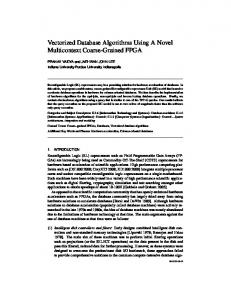
Dec 5, 1995 - Janitor. Fields. Building. Name. House ID. Dorm. Fields. Student ID. Figure 4: Determining the join fields and validity of generated queries.
Anytime Database Algorithms Joshua Grass, Shlomo Zilberstein and Eliot Moss Computer Science Department University of Massachusetts Amherst, MA 01003 U.S.A. {jgrass,shlomo,moss}@cs.umass.edu December 5, 1995 Abstract Optimized queries greatly increases the speed in which queries can be answered by a database. Unfortunately, query optimization is computationally expensive. Can query optimization be combined with anytime algorithm techniques to determine the amount of time to spend optimizing a query and the amount to actually spend executing the query on the database? In this paper I create a database optimizer that searches the entire space of possible logically equivalent queries and accurately estimates the cost of evaluating each query. I evaluate the results of the expected query execution time versus query optimization time and show that the resulting graphs exhibit the qualities we want out of a well-behaved anytime algorithm.
1 Introduction As databases increase in size, and the number of users accessing a database at any one time increases, database systems need to optimize computational resources. One effective way of reducing search time is to optimize queries made to the system. Unfortunately, query optimization is a computationally intensive process itself, and may not be worth pursuing completely. Fortunately, query optimization does not need to be executed to completion in order to increase the speed of search. Since query optimization can be written as an iterative function of increasing quality, it may be possible to make query optimization an anytime algorithm. If we did make query optimization an anytime algorithm we would want it to have the properties of a well-behaved anytime algorithm. Not only because the properties themselves are useful, but also because then the performance profile of the query optimization engine could be combined with the performance profiles of functions that use the database results [11, 8]. We could then use an anytime database query engine 1
as a component in more complex anytime systems. A well behaved anytime algorithm has a number of properties: 1. Quality measure: An anytime algorithm must return results that have a measurable quality. 2. Monotonicity: The quality of the results must increase as the function is given more time. 3. Consistency: The quality must be predictable given the input quality and the amount of time the algorithm is allowed to work. 4. Diminishing returns: The increase in quality must be greater in the beginning of execution than towards the end of execution. 5. Interruptibility: The function must not fail if it is interrupted. It must return a usable result at any time during execution. 6. Resumability: The function must be able to be resumed without difficulty. The purpose of this synthesis project is to determine if we can create an anytime query optimizer that has these properties. In this paper I will describe the algorithm that the anytime query optimizer will use, the cost evaluation function, and the results of several experiments on a sample database.
2 The optimizer The optimizer searches through the space of all possible query trees that use the same databases. It eliminates trees that are not possible, and keeps a record of the least expensive tree using an accurate cost function(see section 3) . When the system is interrupted, or the time for optimization has ended, the least expensive query found so far in the search is returned. If evaluation is to be resumed then only three integers need to be stored in order to continue evaluation at a later point. The search space is enumerated and thus there is no chance of looping.
2.1 The language The language used for querying the system is a subset of QUEL. The syntax is:
2
retrieve sort Where:
{into temp}{(field field...)} [from database | where database.field COMP [database.field | constant]] ; database into temp by field ; {} = Optional [A | B] = A OR B temp = a temporary database(will be lost after query) field = a database field database = a database or temp database COMP = Comparison [= | < | > | =] constant = number or string
If a query command does not have an {into temp}then it is assumed to be the output.
This simple language allows a user to make complex queries into a database system that the interpreter can manipulate into a tree structure containing five different node types. Some of these nodes may be pipelined, which greatly speeds up the process of evaluating the node. These node types are: Database – Database nodes open a database file and pass records to a parent node. Since the still has to be read into memory no pipelining out is allowed. Filter – Filter nodes compare a field to a constant. If the field passes the comparison, then the record is passed upward. This node allows pipelining out and will pipeline in if the input allows. Sort – Sort nodes sort an entire database based on the contents of a field. Since a file must be used, no pipelining is allowed into the node, but it can pipeline out. Select – Select nodes allow only certain fields of a record to continue up the tree. This node allows pipelining into itself and out of itself. Join – Join nodes search two databases for fields that are equal. If two records(one from each database) have equal fields, then the concatenation of the two records is passed upward. This node allows pipelining out of itself and may or may not allow pipelining into itself.
2.2 Representation The query interpreter takes a QUEL form query and builds a tree structure. This tree structure is used for optimization, cost analysis and execution of the query. The interpreter uses the temporary database names to connect children to parents. The tree itself contains a double-linked tree with type and argument information.
2.3 The search space Enumeration through the search space requires three indices: A database ordering index, a tree shape index and a sort index. Using these three values a query tree can 3
Database
Filter
File
Sort Field COND constant
Select
Field
Join
(Field Field...) Field
Field
Figure 1: The five different node types and their representation
(first last dorm)
last
retrieve into residence where student.stid = housing.hid retrieve into older where residence.age >= 21 sort older into directory by last retrieve (first last dorm) from directory
age >= 21
stid Student
hid Housing
Figure 2: Converting a query into a query tree be built that contains all possible join and sort configurations. The reason we do not need to consider all possible positions for filter and selection nodes is that they have an optimal position that we can quickly add to the join-sort tree. First the optimizer scans down the tree searching for all of the databases in the query, adding them to a list of databases used. The query optimizer can determine the number of iterations required to completely search the query space from the number of databases used by the original query.
4
2.3.1 Building the join-sort tree The join-sort tree is built by determining an order for the database nodes, combining them together in different tree configurations, and possibly inserting sort nodes between the children of a join and the join node. The order of the initial database nodes is determined by an integer to permutation algorithm. Given n database nodes we have n! potential orderings. The ordering index tells us which ordering we are currently on. We take the index mod n ( o1 ), and select that database node from the original database list compiled when the query is first passed to the optimization function. We than mark that node as taken and take the index divided by n mod n-1( o2 ). Then we select the o2 th database that hasn’t been selected yet. We continue this process until we have an list of database nodes ordered by the ordering index. Just like any permutation ( o1o2 : : : on ) we can easily predict the number of permutations ( n! ) and can generate a list of the permutations.
c
b
a
d
Figure 3: A generated query tree with order index=13 and tree index=4
5
For instance let’s suppose we have a four node list(a b c d) and an index of 13. 0 a
1 b
2 c
3 d
unselected index index mod n ( on ) index / n ordered database nodes database nodes 4 abcd 13 1 3 b 3 acd 3 0 1 ba 2 cd 1 1 0 bad 1 c 0 0 0 badc Once we have the ordering we can determine the tree structure from the tree shape index. Since each database will need to be connected together, there are (n ? 1) join nodes that we will use to build the query. Much like we did the ordering we need to determine what order to combine the nodes. If we look at the node pairs we can see that the enumeration algorithm is almost identical. n
0 a
1 b
2 c
d
We try every permutation of pair selections. This way every tree configuration will be generated.(And unfortunately, so will some extras, see 2.4) To continue our example, let’s suppose that our tree index was 4. n node list index index mod n ( on ) index / n after joining node on and on + 1 cd c 3 badc 4 1 1 ba 2
cd c ba d
1
1
0
d cc d d c
bad
cd c badc 1 ba 0 0 0 For each join node the arguments that specify the two fields that they will compare need to be determined by the optimization algorithm. This is the first of many functions that will use the original query tree as a guide to determine how to act. In this case we need to determine which fields to place on the branches of the join nodes so that the query is logically equivalent. There will also be cases where this is not possible and we can disregard the tree. We need to start maintaining information about each node’s field list(which fields are in the record), if it is a database this will simply be read from the file and stored in the node data. If it is a join node then the field list will be the concatenation of the field lists of the two child nodes. To determine the two fields for the join node arguments we have to look at each join node in the original query. If there is a join node in the original query in which the join arguments are in the field lists of both nodes of the generated query, then we have a connection and we can use those same arguments. Figure 4 makes this a bit more clear. 6
The original query tree Fields Student ID Name House ID
5
Dorm Building Janitor
Fields Student ID
Dorm
Name House ID
Building
4
Janitors
Dorm Student ID Student
House ID Housing
Fields Student ID
Fields House ID
Name
Dorm Fields Student ID
A valid generated tree
An invalid generated tree
Name House ID Dorm Building
2 Fields Building
Fields Building Janitor
Janitor House ID
Janitor House ID Dorm
Student ID
1
Students
Fields Student ID
3
Housing
Dorm
Name Building Janitors Fields Building Janitor
Fields House ID
Dorm
No match
Housing
Janitors
Fields House ID
Fields Building Janitor
Dorm
No match Students Fields Student ID Name
Figure 4: Determining the join fields and validity of generated queries When generating the valid tree, on the lower left, we first try to determine the argument fields for node 1. To do this we start scanning the original query to see if any of it’s join nodes have two arguments that are in both of the field lists of the generated join node’s children. When we look at node 5 in the original query tree we see one of it’s arguments is dorm, and the other is building. Since dorm is in the field list of one of node 1’s children(Housing), and building is in the other child’s field list(Janitors) we know that this is a valid join node. Since the original was looking for equal dorms and buildings, our graph will remain equivalent if it has the same arguments in it’s join node between these two databases. Node 2 of the valid tree is also valid. As we search each join node of the original query we find a node(4) in which student id and house id are joined. Since student id is in the field list of the student database, and house id is in the field list of the janitor-housing join, we can use these arguments in node 2. Node 3 in the invalid generated tree cannot be joined because no node exists in the original query in which two fields from either of these field list are ever joined. Since
7
these two database do not share any direct connection the node is invalid. b
a
c
Sort index=9
d
b
d
Sort index=9
4 even c Field
9 odd a
d
Sort index=2
Sort index=0 0 even
2 even
0 even
1 odd
b
d
Field
b Field
c Field
c
a Field
a
Figure 5: The sort node with a sort index of 9 Finally, we need to add the sort nodes using the sort index. We can place a sort node on either branch of every join node. Since we know what field the join will use for that database, we know which field to sort the database by if we decide to sort. We can either sort or not sort the 2(n ? 1) branches for (n ? 1) join nodes. This gives us a sort index that ranges from 0 to 22(n?1). The implementation for the sort insertions is simple: when two nodes are joined, if the sort index is odd then a sort node is added to the left branch. Then the sort index is divided by 2 and if it is odd a sort node is added to the right branch, and then the index is divided by 2 again. The algorithm does this for each join node it creates. 2.3.2 Adding filters Adding filters is relatively easy since there is an optimal location for filters to be placed. Since filters are always pipable and either reduce the size of a database or don’t effect it, we simply push each filter we find down until it reaches the database. At execution time, the filter node can be executed as the database is loaded in. In figure 6 you can see the process by which the filter is pushed down the tree until a database is found.
8
A valid generated tree
Fields Student ID Name House ID Dorm Building Janitor
1 Fields Building
House ID
Janitor House ID
Student ID
2
Dorm
Students
Fields Student ID Name
Building
3
Dorm Housing
Building > "M" Fields House ID Dorm Janitors Fields Building Janitor
Figure 6: A filter going down a generated query tree When there is a choice between two children(a join node) the filter can use the field lists of each child to decide which branch to continue down. The child that has the filter’s field argument(in the figure 6 “building”) in it’s field list is the correct node to follow. In figure 6 the circled numbers trace the path of the filter until it reaches the database node, Janitors. 2.3.3 Adding selection A selection node contains a list of fields that are formed into a new record that is passed to the parent of the selection node. The selection node for a tree generated by the optimization algorithm is created from the field list of the top node of the original query. Since selections reduce the size of a database, we want to push the selection commands as far down as possible, to reduce the amount of information through the system. The selection node begins at the top of the generated query, as it proceeds downward it can encounter join, sort, filter and database nodes. In each situation it acts slightly differently. Figure 7 has a visual example of each of the three cases described below. The simplest case is when the selection node encounters a database node. If it’s
9
Database (name age)
(name age)
(name age)
Current selection node
Current selection node Database
Database
Database
Fields
Fields
Fields
Database Fields
name
name
name
name
age
age
age
age
student id
student id
Sort or Filter (name age) (name age) (name age)
age > 21
Current selection node
Current selection node
dorm age > 21
dorm
(name age)
Current selection node (name age dorm)
Current selection node
Join (name dorm)
(name dorm)
Current selection node
name
Fields name age
guest-list
Fields
name
(name)
guest-list
(guest-list dorm)
guest-list dorm
Current selection node
Figure 7: A selection node encountering other nodes field list exactly matches the database field list, then no fields are to be removed and the selection node is useless. In this case it is not added to the query. If the selection node does eliminate some fields then the selection node is added to the database immediately after the database node. The sort and filter cases both effect the selection node the same way. First the argument field of the filter or sort are checked to see if they are a part of the selection nodes field list. If they are, then the selection node moves on to their single child node with no change to itself or the query. If the field argument of a sort or filter node is not in the selection node’s field list, then the selection node is inserted directly above the sort or filter node and a copy of the selection node with the sort or filter node’s argument added to the selection list is propagated to the node’s child. This way, the information needed for the sort or filter node will be in the database for it, but removed after it is no
10
longer needed. The final case is a join node. When a selection node encounters a join node on it’s path to the bottom of the query tree, it divides into two selection nodes. Each new selection node contains a selection field list of all the fields that are both in the join child’s field list and in the original selection node field list. Also, if the argument field for the join is not in the field list of the new selection node, then it is added, and the original selection node is inserted directly above the join.
2.4 Search space size In order to build all possible tree configurations and possibly add a sort to each branch of each join, we have a search space of size: 2(n?1) |{z} | ?{z } | {z } Orders Sorts n!
(n
1)! 2
(1)
Trees
Where n is the number of database nodes. It has recently come to my attention that I have over searched the tree space. For instance, I consider
a
b
c
d
! abb
a
b
c
d
!
c
a
b
b cdb ! abb cdb ! abd b cdb b ! abb cdb ! abd cd d
to be two separate cases, when in actuality they are not. The actual formula for the tree search space is:
1
n
�
2n ? 2 n?1
�
I have not yet been able to add this new enumeration to the tree construction algorithm.
3 The cost function The cost function gives an approximation of the amount of time required to execute a query. In order to be as accurate as possible it keeps track of the database size and configuration at each node in the tree. In order to give the most reliable estimates possible for join and filter nodes(other then actually doing the computation) the cost function uses histogram representations of the database to predict the number of hits [5]. Each node contains information about the database that will be output by that node. This information will generally become less and less accurate the further away a node is from a database node, where it can read this information from the database header. Number of rows – The estimated number of rows in the database at this node. 11
Number of columns – The number of columns in the database. Size – The estimated size(in bytes) of the database. Pipable – Whether information from this node can and is being piped upward, instead of being stored in a temporary file. Field list – A list of the fields in the database. Unique – An estimate of the number of unique values in each field. Sorted – Whether the field is sorted. Sometimes more then one field can be sorted due to joins. Unit cost – The cost to execute this one node. Total cost – The cost to execute the child nodes and this one. Using the above node information, histograms of the databases, and the assumption that field values are independent, Kooi [5] has shown that this cost model is very accurate. The cost model is based on the number of blocks written and read during the course of the query.
3.1 Database Database nodes do not load information, and are thus not pipable. They open a file pointer that the parent node may use for loading individual records or for sorting. If a database did load information, a sort node would just have to ignore it. This way disk-time is only used if needed. Number of rows read from file header Number of columns read from file header Size read from file header Pipable false Field list read from file header Unique read from histogram Sorted read from file header Unit Cost 0
3.2 Selection Selection has a very simple cost model. If the input node is pipable, the cost is 0 since it can edit records in memory and pass each up one at a time to the parent node. If the input node is not pipable, then the cost is equal to loading in the file.
12
Number of rows Number of columns Size Pipable Field list Unique Sorted Unit Cost
same as input node same as number of selection fields calculated from rows and columns true equal to selection list same as input node same as input node size 0 if pipable, input blocksize if not pipable
3.3 Filters Since filters do not change the order of the database and only need to look at one record at a time their cost is 0 if the input node is pipable. Otherwise, they must load in the file. Number of rows see below Number of columns same as the input node Size calculated from rows and columns Pipable true Field list same as input node Unique see below Sorted same as input node size Unit Cost 0 if pipable, input blocksize if not pipable To determine the number of rows for a filter function the cost function must descend down the query tree until it finds the database node that contains the field that filter uses. Once this database is found, the histogram for the database is accessed to determine the number of rows that would be passed through the filter if it were being applied directly to the database. If it is not, then the ratio between the number of rows in the database and the number of rows of the input node is used to calculate the estimated number of rows in the filter. As long as independence is true this should be an accurate estimate. “Database” is the original database. rows = hits(f ilter; database
histogram )
rows rows
database input
The number of unique values is also calculated from a ratio of the filter’s number of rows and the input node’s number of rows. The number of unique values for the field the filter uses for comparison is calculated from the histogram.
3.4 Sorting Sorting is quite expensive and unless it helps several joins, it is not worth the trouble. It also must be done on disk and has to write records completely out to a file if it is receiving piped input. 13
Number of rows Number of columns Size Pipable Field list Unique Sorted Unit Cost
same as input node same as input node same as input node false same as input node same as input node argument field is true inputsize (if piped to sort) + blocksizenumRows input size + blocksize
inputsize blocksize
If the data is piped to the sort node then the data must be written out to the disk before sorting can be done. Since sorting requires access to the entire database and not just one row at a time.
3.5 Joining We will refer to the left input node as left, and the right input node as right. The original databases for the left and right database are referred to by lo and ro. Number of rows see below Number of columns left.columns + right.columns Size calculated from rows and columns Pipable true Field list left field list concatenated with the right field list Unique see below Sorted see below Unit Cost see below Determining the number of rows for join is very similar to how the rows are determined for a filter. First the original left and right databases are found. Then using the histograms the number of hits is determined. Assuming that field values are independent, the new number of rows for the join node is determined by this formula: rows = hits(lef t
histogram ; righthistogram )
rows rightrows lorows rorows
lef t
The number of unique values is calculated from the input node’s number unique values and the new number of rows. The unit cost is determined by several factors, depending on whether the left or right input nodes are sorted, piped and/or unique.
14
left sorted yes
right sorted yes
left piped yes
right piped yes
left unique yes
cost
yes
yes
yes
no
yes
leftsize blocksize
yes
yes
no
yes
yes
rightsize blocksize
yes
yes
no
no
yes
leftsize rightsize blocksize
yes
yes
yes
yes
no
2
yes
yes
yes
no
no
bufSize(leftrows ? leftunique) bufSize(leftrows ? leftunique )
yes
yes
no
yes
no
2
yes
yes
no
no
no
leftsize bufSize(leftrows ? leftunique ) + blocksize
no
–
yes
–
–
rightsize blocksize
leftrows leftrows
0
+
leftsize bufSize(leftrows ? leftunique) + blocksize
–
no
yes
–
–
rightsize blocksize
no
–
no
–
–
rightsize blocksize
leftsize leftrows + blocksize
–
no
no
–
–
rightsize blocksize
leftsize leftrows + blocksize
Where bufSize is the average amount of re-reading you’ll need to do in a non-unique right sided database. This value is: buf Size =
cols f ieldlengthrightrows rightunique blocksize
right
3.6 Calculating the tree cost Calculating the cost of a query involves recursively calculating the cost of children nodes on the query tree. At the end of the calculate cost function the cost of writing the results back to the disk must also be added to determine the final cost of the query. This cost is:
totalcost + f ractopsize blocksize
top
4 Experiments In this section I demonstrate the anytime optimizer working on a single problem and on several classes of problems. The first experiment shows the output of the optimizer running to completion, displaying the current, best and worst queries. The second experiment shows two performance profiles that were created when the optimizer was run on groups of queries that are of two different sizes. From these we can evaluate if the anytime query optimizer is well-behaved as described in the introduction.
15
4.1 The database For the following experiments, I created a small database based on a college record system. There are five databases: Student – The student database contains a first and last name, a student id and the age of the student. Class – The class database contains the title of a class, a class number, the building and room it is in, and the time of the class. Enrollment – The enrollment database contains an enrollment id(eid) and an enrollment class number(eclass). Housing – The housing database contains the housing id(hid) the dorm and the apartment number of a student. Clean – The cleaning database contains information about the structure to clean (building or dorm) the team that cleans it every night and what time they usually start. Database Student Class Enroll Housing Clean
Fields first last stid age title clnum building room time eclass eid hid dorm apt structure team time
Rows 25 10 94 25 8
Blocks 3 2 5 2 1
Summary of the databases, the fields, the size in rows and the size in file blocks
4.2 An example query For the first experiment I ran the query optimizer on the following query: retrieve retrieve retrieve retrieve retrieve
into temp where student.stid = housing.hid into temp2 where temp.age >= 20 into temp3 where temp2.stid = enroll.eid into temp4 where temp3.eclass = class.clnum (last building time) from temp4
Here is the output of the anytime optimizer evaluating the original query: Building the query tree... Calculating the cost of the tree... Select (last building time) from: eclass = clnum stid = eid age >= "20" stid = hid Database student Database housing Database enroll Database class Total cost: 226
Cost:0/222 R:51 C:3 P:1 S:1792 Cost:102/222 R:51 C:14 P:1 S:8084 Cost:70/120 R:51 C:9 P:1 S:5204 Cost:0/50 R:14 C:7 P:1 S:1174 Cost:50/50 R:25 C:7 P:1 S:2032 Cost:0/0 R:25 C:4 P:0 S:1174 Cost:0/0 R:25 C:3 P:0 S:888 Cost:0/0 R:94 C:2 P:0 S:2189 Cost:0/0 R:10 C:5 P:0 S:620
16
Figure 8: A performance profile for a single query The optimizers best response was: Select (last building time) from: Cost:0/87 R:51 C:3 P:1 S:1781 stid = eid Cost:0/87 R:51 C:5 P:1 S:2925 Select (last stid) from: Cost:0/35 R:14 C:2 P:1 S:358 stid = hid Cost:14/35 R:14 C:3 P:1 S:523 Sort by stid Cost:16/19 R:14 C:2 P:0 S:331 Select (last stid) from: Cost:0/3 R:14 C:2 P:1 S:349 age >= "20" Cost:0/3 R:14 C:3 P:1 S:514 Select (last stid age) from: Cost:3/3 R:25 C:3 P:1 S:888 Database student Cost:0/0 R:25 C:4 P:0 S:1174 Select (hid) from: Cost:2/2 R:25 C:1 P:1 S:316 Database housing Cost:0/0 R:25 C:3 P:0 S:888 Sort by eid Cost:0/52 R:94 C:3 P:1 S:3238 Select (building time eid) from: Cost:0/52 R:94 C:3 P:1 S:3238 clnum = eclass Cost:50/52 R:94 C:5 P:1 S:5328 Select (building time clnum) from: Cost:2/2 R:10 C:3 P:1 S:378 Database class Cost:0/0 R:10 C:5 P:0 S:620 Database enroll Cost:0/0 R:94 C:2 P:0 S:2189 Total cost: 91
The optimizers worst response was: Select (last building time) from: Cost:0/1743 R:51 C:3 P:1 S:1772 hid = stid Cost:125/1743 R:51 C:5 P:1 S:2916 Select (hid) from: Cost:2/2 R:25 C:1 P:1 S:316 Database housing Cost:0/0 R:25 C:3 P:0 S:888 Sort by stid Cost:265/1616 R:51 C:4 P:0 S:2304 Select (last building time stid) from: Cost:0/1351 R:51 C:4 P:1 S:2344
17
stid = eid Cost:98/1351 R:51 C:5 P:1 S:2916 Select (last stid) from: Cost:0/3 R:14 C:2 P:1 S:349 age >= "20" Cost:0/3 R:14 C:3 P:1 S:514 Select (last stid age) from: Cost:3/3 R:25 C:3 P:1 S:888 Database student Cost:0/0 R:25 C:4 P:0 S:1174 Sort by eid Cost:672/1250 R:94 C:3 P:0 S:3204 Select (building time eid) from: Cost:0/578 R:94 C:3 P:1 S:3247 eclass = clnum Cost:89/578 R:94 C:5 P:1 S:5337 Sort by eclass Cost:475/475 R:94 C:2 P:0 S:2173 Database enroll Cost:0/0 R:94 C:2 P:0 S:2189 Sort by clnum Cost:12/14 R:10 C:3 P:0 S:350 Select (building time clnum) from: Cost:2/2 R:10 C:3 P:1 S:378 Database class Cost:0/0 R:10 C:5 P:0 S:620 Total cost: 1747
Cost R C P S
Cost of executing current node / cost of executing current branch Estimated number of rows after executing this command Estimated number of columns after executing this command Is the output pipable to the parent command? (1–Yes, 0–No) Estimated size of the database after executing this command, in bytes The optimizers analysis of the database at each operation
The performance profile in figure 8 exhibits the characteristics that we want, namely, monotonicity and diminishing returns. The improvement from the original query to the optimized one was large (50% of the execution time was saved) and we can see that the optimizer can be allocated a large amount of time and still make up for it in performance savings. These databases are also small and the effects on a larger database would be even more noticeable.
4.3 Performance profiles The performance profiles in figure 9 show the characteristics that we want out a performance profile for an anytime algorithm. Especially the performance profile for the four database node graph. We can see monotonicity and diminishing returns. Also important for practical reasons is that the performance profile points are fairly clumped together, this means that the performance profile’s standard deviation is small, meaning the execution savings is more predictable given an optimization time.
5 Conclusion The anytime query optimizer that I created demonstrates the six principles of a wellbehaved anytime algorithm that we were looking for:
18
Figure 9: The performance profile for a group of 3 database queries(left) and for a group of 4 database queries(right) Quality Measure – The work of Kooi’s [5] paper demonstrates that using histograms and given independence between variables the query cost function is very accurate. Monotonicity – The code enforces monotonicity by keeping the lowest cost query in memory in case of interrupt and for comparison with new queries. Consistency – Here we look at the small standard deviation for the performance profile of the class of queries. The class performance profile generator(which we used to build the performance profiles of a given size) generates queries of all possible configurations of the same size. Diminishing returns – Again the class graphs show diminishing returns. Interruptibility – The optimization algorithm, by maintaining the highest scoring query in memory, can be interrupted and return the best query so far. Resumability – Since the query optimizer only needs three integers to remember it’s state, it is very easy to resume computation. Thus all six criteria for the anytime optimizer begin a well-behaved anytime algorithm have been met. Of course, with an improved search function, the performance profiles would most likely be smoothed. Unfortunately, I not sure what the cost of an improved search function will be in terms of Resumability and memory requirements. Maintaining a list of previously explored nodes would be prohibitively expensive. I believe the correct approach is to try to optimally order the database nodes initially, so that the same permutation mechanism could be used. An anytime query optimizer will be extremely useful in resource-bounded reasoning problems with databases. 19
6 Future work There are still many avenues to explore in anytime query optimization. One of the first is to try and determine an effective search technique so that we can make the performance profile exhibit the characteristics(monotonicity and diminishing returns) we want. The optimizer already has the other four characteristics from the algorithms we use. A more long term goal would be to utilize meta-knowledge about the structure of the database. For instance, in our example database perhaps each year all new students are placed in the same dorm. We could easily infer information about the location of all of the students for free if we knew their year in school. This semantic knowledge adds another area in which queries might be optimized. Partial evaluation could also be investigated. By extending my querying language to given utility to the number of results and an ordering, the query optimizer could determine how much time to spend on query execution. For example, if I wanted to know the GPA’s of students but I mostly wanted the people with the lowest GPA’s, the system could be expanded to find the most relevant records first depending on the resource constraints. Currently, not much work has been done combining resource-bounded reasoning and database systems. Many problems still need to be addressed and solved.
Acknowledgements This work was partially supported by the University of Massachusetts under a Faculty Research Grant and by the National Science Foundation under grant IRI-9409827.
References [1] M. Boddy and T.L. Dean. Solving time-dependent planning problems. In Proceedings of the Eleventh International Joint Conference on Artificial Intelligence, pages 979–984, Detroit, Michigan, 1989. [2] Johann Christoph Freytag. A rule-based view of query optimization. In Proceedings ACM-SIGMOD, pages 173–180. ACM, 1987. [3] Goetz Graefe and David J. DeWitt. The exodus optimizer generator. In Proceedings ACM-SIGMOD, pages 160–172. ACM, 1987. [4] Joshua Grass and Shlomo Zilberstein. Programming with anytime algorithms. In Anytime Alogrithms and Deliberation Scheduling, pages 22–27, Montreal, Canada, 1995. IJCAI-95.
20
[5] Robert Philip Kooi. The Optimization of Queries in Relational Databases. PhD thesis, Case Western Reserve University, 1980. [6] Shashi Shekhar, Jaideep Srivastava, and Soumitra Dutta. A fromal model of tradeoff between optimization and execution costs in semantic query optimization. In Proceedings of the 14th VLDB Conference, pages 457–467, Los Angeles, California, 1988. [7] Sreekumar T. Shenoy and Z. Meral Ozsoyoglu. A system for semantic query optimization. In Proceedings ACM-SIGMOD, pages 181–195. ACM, 1987. [8] S. Zilberstein. Operational Rationality through Compilation of Anytime Algorithms. PhD thesis, University of Califonia, Berkeley, 1993. also Technical Report No. CSD-93-743, Available on-line at http://anytime.cs.umass.edu/�shlomo. [9] S. Zilberstein and S. J. Russell. Efficient resource-bounded reasoning in at-ralph. In Proceedings of the First International Conference on AI Planning Systems, pages 260–266, College Park, Maryland, 1992. [10] S. Zilberstein and S. J. Russell. Anytime sensing, planning and action: A practical model for robot control. In Proceedings of the Thirteenth International Joint Conference on Artificial Intelligence, pages 1402–1407, Chambery, France, 1993. [11] S. Zilberstein and S. J. Russell. Optimal composition of real-time systems. Artificial Intelligence, 1995.
21