Benchmarking Punctuated Anytime Learning for Evolving a Multi-Agent Team’s Binary Controllers
H. JOSEPH BLUMENTHAL, GEORGE MASON UNIVERSITY, USA
[email protected] GARY B. PARKER, CONNECTICUT COLLEGE, USA
[email protected]
ABSTRACT Punctuated anytime learning (PAL) is a system that can be used for evolving cooperative teams of agents. PAL applied to evolving multiple populations is a kind of cooperative coevolutionary algorithm (CCEA). Here we compare PAL to a canonical genetic algorithm (GA) on a widley used GA benchmarking optimization function called the Rosenbrock function. The Rosenbrock function was chosen for experimentation because it is a highly non-linear function and difficult to optimize. Results are shown from a variety of experiments with different dimensionalities of the Rosenbrock function. These findings are discussed in the context of evolving binary controllers for mutli-agent cooperative teams of robots.
KEYWORDS: Evolutionary Algorithms, Optimization, Co-evolution, Robot Control, Learning 1. INTRODUCTION In recent years there has been much interest in studying teams of robots. One major reason for this focus is their wide range of potential applications. Multi-agent teams can be used for a variety of tasks including search and rescue missions and toxic waste cleanup. Teams of cooperative agents have great potential to accomplish goals that single agents cannot complete alone. A design issue facing any practitioner when organizing teams of agents is the question of whether or not specialization of roles is beneficial for solving a particular problem. If every member of a team uses identical controllers the team is said to be homogeneous. There are many problem domains in which a single set of behaviors is sufficient for a team of agents to accomplish the goal. When members of a team have unique control systems, the team is said to be heterogeneous. We choose to focus on methods that produce heterogeneous teams because a team exhibiting specialized behaviors can often find more appropriate solutions to complex tasks. One system devised for producing heterogeneous teams of agents is the cooperative coevolutionary algorithm (CCEA) [1]. The standard genetic algorithm initializes a pool of candidate solutions in the form of random bit-strings and probabilistically applies mutation and recombination operators to drive the parallel search. However, a CCEA operates by decomposing the solution into two or more coevolving populations. We have developed a particular implementation of CCEA that uses punctuated anytime learning (PAL). Our research has established PAL’s ability to evolve heterogeneous teams of agents for non-trivial tasks while reducing computation time [2]. In this paper, we compare our PAL system to a standard GA on a commonly used benchmarking test function to show the advantage of using PAL for evolving complex multi-agent coordination strategies. We will start by discussing some previous work germane to our research followed by a detailed description of the PAL method. We will then outline our experiments and discuss the results. We will then finish with our conclusions and plans for future research.
2 PREVIOUS WORK Many different methods have been used to learn the control and coordination of cooperative teams of agents. Our research focuses on evolutionary approaches to learning cooperative behaviors. We specifically explore cooperative coevolutionary approaches to evolving teams of agents. We have developed a particular coevolution system that is a based on a traditional evolutionary algorithm (EA). Our primary interest in this work is to compare our coevolutionary method against a standard genetic algorithm. To serve as a base of comparison we use a common benchmarking function for evolutionary algorithms. One example of learning to control a heterogeneous team is the work done by Luke and Spector [3]. In this research, they use an EA to evolve team members using a single population. In this model, a single member of
the population contains the perspective team members. In order to test their methodology, they used a simulated predator/prey scenario that was designed to be an abstraction of the African Serengeti. In this research a team of four agents represented as “lions” cooperate to capture a fifth agent representing a “gazelle”. This method of evolving all of the team members in a single population is the method to which we will compare our method. The cooperative coevolutionary algorithm, (CCEA) was originally proposed by Potter and De Jong [1]. This coevolutionary technique is very similar to ours. The main feature of the CCEA is that each member of the team is evolved in a separate population. The CCEA method uses the best individual found during the previous generation of training from each population to evaluate any perspective team member. Potter and De Jong also experimented with increasing the number of collaborators used to evaluate an individual. In their investigation, they tested both the best individual and another random collaborator from its own population. Potter, Meeden, and Schultz applied this system to a robot shepherding task [4]. The problem involved multiple shepherding agents controlled by neural networks to coordinate to herd sheep into a corral. Wiegand, Liles, and De Jong, examined pertinent issues to coevolution when increasing the number of collaborators at trial time [5]. One of their conclusions was that the most important factor in the success of coevolution is the number of partners used to test the candidate solution. This fact may seem rather intuitive but it highlights a central issue in coevolution. While the number of collaborators tested increases linearly, the number of evaluations expended increases exponentially. Our method of coevolution has similarities to the CCEA described above. In subsequent sections of the paper we describe in greater detail the mechanics of the algorithm. We have applied our method of coevolution to a box-pushing task and a predator/prey scenario with good results. From the research presented in this paper, we hope to better understand how our method extends to a large number of populations and how our method compares to a standard genetic algorithm.
3 Evolutionary Algorithms for Learning Cooperation An evolutionary algorithm is essentially a massive parallel search strategy that is loosely based on Darwin’s theory of natural selection. In an EA a population of candidate solutions, traditionally represented as binary strings, is randomly generated. A particular metric called a fitness function is then used to evaluate all of the individuals (bit-strings) in the population. Using this measure of fitness, members of the population are stochastically selected to apply genetic operators. Though there exists an abundance of genetic operators, the two most commonly used are recombination and mutation. In recombination, two or more individuals are selected from the population and sections of each individual’s bit-string are combined to form a new individual. A mutation operator is often used after recombination has produced a new individual to probabilistically flip a particular bit in the new individual’s bit string. This process of applying genetic operators is repeated until a new population of individuals has been created. The process of evaluating a population and creating a new population is referred to as a generation of learning. The EA continues this process for a set number of generations or until a pre-determined level of fitness is obtained. Our punctuated anytime learning (PAL) method of coevolution was originally created to solve very difficult cooperative coevolution problems. The algorithm is based on the anytime learning system developed by Grefenstette and Ramsey and was later renamed continuous embedded learning [6]. The continuous embedded learning architecture is comprised of an onboard learning system, an internal model of the environment, and a monitor. The monitor’s purpose is to detect discrepancies between the internal model and the external environment. When the monitor detects that a factor in the environment has changed, it updates the robot’s internal model. Parker developed punctuated anytime learning to strengthen offline genetic algorithms. The basic idea is that although an offline genetic algorithm cannot get continuous updates triggered by a monitor component, it can update its simulation model at consistently spaced generations of training called punctuated generations. PAL updates take the form of running tests on the real robot at these punctuated generations which result in periods of accelerated fitness growth. The algorithm then uses this information for fitness biasing or the coevolution of model parameters [7]. This is very similar to the way our learning system behaves except that the updated information that our learning algorithm receives is a more accurate model of the populations that are coevolving. At the punctuated generations an alpha individual is selected as the best representative of the nature of its population. Our algorithm for alpha selection can be described as follows:
1. For each population select a random sample of S individuals. 2. For each individual in each population, test the individual using the S partner combinations collected from all of the other populations. 3. Average the vector of fitness scores resulting from testing the S partner combinations. 4. For each population select the individual with the highest fitness relative to its own population members. During non-punctuated generations, the alphas selected from the last punctuated generation are used as collaborators for evaluating individuals. When we first developed our method, we wanted the most accurate alpha individuals as possible so we set the sample size of collaborators used for alpha selection to the size of each population [2]. This meant that at each punctuated generation we were testing every single possible partner combination. This method was applied to a simple box-pushing task with only two agents. While this method worked well for small numbers of populations like two, it was too computationally expensive for tasks requiring three or more partners. For example, if there was a task requiring 4 populations with 100 individuals in each population, a single round of alpha selection would incur 1004 or 100,000,000 evaluations. This level of computation is unacceptable. We reasoned we could still get an accurate estimate of a population by sampling less than an exhaustive search of partner combinations (Parker and Blumenthal 2002b). To get a clearer picture of how the PAL with sampling method compares to the original PAL method, it is helpful to see Equation 1. For a task requiring P populations, of I individuals each, and a sample size of S, the number of evaluation for alpha selection becomes:
P*(I*SP-1)
(1)
If there are 4 populations with 100 individuals each and a sample size of 2 a single round of alpha selection would expend 3,200 comparisons. Looking back at our original PAL method we have reduced the number of computations for alpha selection from 100,000,000 to only 3,200. In this example PAL with sampling has reduced the number of computations by a factor of 31,250 times. After discovering the effectiveness of our new method for saving computation time, we tested several sample sizes on our box-pushing problem to establish their properties [8]. In order to prove PAL’s capacity to learn challenging coordination problems we applied our new sampling method to two different predator/prey problem domains with success [9].
4 THE ROSENBROCK FUNCTION The purpose of this paper is to compare our coevolution method PAL to a standard GA on a benchmarking function. The function we chose for comparison is the Rosenbrock function. The Rosenbrock function has been frequently used to test the performance of a GA as part of the De Jong test suite [10]. We believe Rosenbrock to be an excellent benchmarking function because it has been extensively studied across GA literature and has even been used to test the strength of CCEAs [1]. The Rosenbrock function is presented as Equation 2. The Rosenbrock function is traditionally defined in terms of a two variable function optimization problem. However to grant flexibility in our experiments we wanted to test the function with a wider range of dimensionalities. To accomplish this we created our own N dimensional extension. Our N dimensional extension of the Rosenbrock function is shown as Equation 3.
f ( x1 , x2 ) = 100( x2 ! x12 ) 2 + (1 ! x1 ) 2 n
[
f ( x) = ! 100( xi " xi2"1 ) 2 + (1 " xi "1 ) 2 i =2
(2)
]
(3)
The Rosenbrock function has a global minimum of 0. This minimum is reached when all input variables are 1.0. The traditional initialization range for a Rosenbrock function variable is between -2.048 and 2.048. We selected the Rosenbrock function because it is a difficult function to optimize. The characteristic of the Rosenbrock function that presents difficulty is the high level of variable interaction or epistasis present in the
function. The level of epistasis between variables becomes clear when Equation 2 is expanded out in Equation 4. f ( x1 , x2 ) = 100 x14 + 100 x22 ! 200 x2 x12 + x12 ! 2 x1 + 1
(4)
Examining the terms in Equation 4, it is clear that the function is not linearly separable meaning that the algorithm cannot independently optimize terms in the equation, instead it must capture the variable interactions to minimize the function. To get a feel for the difficulty of the Rosenbrock function it is helpful to look at examples of its local minimums in Table 1.
Inputs
(0,0)
(0,1)
(1,1)
(-1,1)
Output
1
101
0
4
Table 1: A set of sample input and resulting output values for the Rosenbrock function. Notice how the functions local minimum draw the search away from the global minimum. The Rosebrock function has several deep local minimums which become substantially deeper when considered in more than two dimensions. It is very easy for algorithms to get stuck in the deep local minimum of (0,0). The Rosenbrock function tends to lead searches away from the global minimum because the input (0,0) gives a good fitness of 1 but the input of (0,1) gives a large fitness of 101. The same is true for the local minimum of (-1,1) which gives a good fitness value of 4.
5 IMPLEMENATATION OF THE GA AND PAL The implementations of both the GA and the PAL were meant to share as many similarities as possible in order to make a fair comparison. Both algorithms used binary representations with a genotype to phenotype mapping over 16 bits. It should be noted that we are aware that an evolutionary strategy with real valued representation is a more effective search, indeed GAs are not function optimizers [11]. Our primary concern is to have a fair comparison between the two algorithms instead of focusing on the best representation to solve the problem. Our primary goal is to test the relative strengths of the two algorithms for evolving binary robot controllers. The major difference in the implementation of the GA and PAL is the encoding of their respective chromosomes. In the implementation of the GA all perspective solutions are represented in a single population. Each chromosome in the GA’s population contains all N variable inputs to the Rosenbrock function. The implementation of PAL is quite different. In this case, each function input variable has its own population. Figure 1 illustrates this fundamental difference using an example of a two variable function input with a population size of five. Aside from the difference in representation, both algorithms share the same parameters. Both implementations have a population size of 100 individuals, use single point crossover, bit-flip mutation, roulette wheel parent selection, with an elitist strategy where the best individual from each population is
PAL
GA Pop (x1,x2) (x1,x2) (x1,x2) (x1,x2) (x1,x2)
Pop 1 x1 x1 x1 x1 x1
Pop 2 x2 x2 x2 x2 x2
Figure 1: Shown above are the different implementations of the GA and PAL shown with a population size of five.
automatically placed with the offspring. The probability of mutation is one out of sixteen corresponding to 1/L where L is the number of bits in the genotype. Additionally, the PAL method uses a sample size of two and selects new alphas every other generation.
6 RESULTS In our experimentation we wanted to try a range of dimensionalities to determine the strength of the PAL method compared to the standard GA. We decided to test the two algorithms on a two, five, and ten variable Rosenbrock function. Figure 2 shows a best-so-far plot of the performance of these two algorithms. In Figure 2, the y-axis represents the fitness of the best-so-far and the x-axis shows the number of evaluations incurred. Each data series is averaged over 10 independent tests of each algorithm. The dashed line is the plot for the standard GA and the solid line is the plot for the PAL algorithm. One of the most noticeable differences between the two algorithms is their starting points at evaluation zero. The PAL algorithm invariably starts at a much worse fitness. This is explained by the fact that PAL begins by testing the random samples for alpha selection. In this process at evaluation zero, there is an overwhelming probability that a poorly fit collaborator will be chosen causing a very poor fitness average. From examining Figure 2, it is clear that for a two variable minimization the standard GA outperforms PAL, though by evaluation 5,000 PAL reaches the same level of fitness. This is a fairly easy problem to solve and the GA must only sequence 32 bits. What happens when the GA has to sequence a larger number of bits in order to minimize the function? Figure 3 shows the two algorithms on a five dimensional extension of the Rosenbrock function. It is easy to see that the PAL algorithm quickly passes the GA’s fitness level. It follows that the GA would have greater difficulty in sequencing five variables than two variables. 0.8
0.7
0.6
Fitness
0.5
0.4
0.3
0.2
0.1
0 0
1000
2000
3000
4000
5000
Evaluations
Figure 2: Two best-so-far plots showing the comparison between the standard GA (dashed line) and the PAL method (solid line) for minimizing the two variable Rosenbrock function. Each line is the average of 10 independent test runs.
50
45
40
35
Fitness
30
25
20
15
10
5
0 0
20000
40000
60000
80000
100000
Evaluations
Figure 3: A best-so-far plot comparison of a five variable Rosenbrock minimization problem. The dashed line represents the GA’s performance and the solid line shows PAL’s performance. In the case of the two variable Rosenbrock function the GA needed to sequence only 32 bits, but it must now sequence a string containing 5 variables of 16 bits each giving a total of 80 bits. The graph shown in Figure 4 reinforces the point that as the number of input variables increases it increasingly stifles the GA’s performance. In this case the GA has to sequence 160 bits. Figure 4 plot lines are each averaged over 10 independent test runs of the algorithm. Although the point x = 0 can not be shown in Figure 4, the GA starts with an average fitness value of 786.55 and PAL starts with a much worse fitness of 1979.73. Examining Figures 2, 3, and 4 give a clear picture of a trend developing in the data. The trend shows that as the number of dimensions of the Rosenbrock function increases so PAL’s relative advantage over the GA. One quality that should be noted is that when the PAL method is run out for a large number of evaluations it usually forges ahead until the global minimum is reached. Up to this point in the discussion we have merely presented the graphs and spoke in vague terms about which algorithm performs “better”. The term “better” is very subjective and it would be helpful to discuss the graphs based on a specific criteria. We will define two different criteria by which to measure the algorithms performance. One way to measure two algorithms’ performances is to evaluate their relative performances given a fixed budget of evaluations. Using this criteria, the question becomes “Given a fixed budged of evaluations to spend, which algorithm will give a more accurate solution?” A second standard for comparing multiple algorithms’ performances is a race to a particular solution quality. Using this measure of performance the question becomes “Which algorithm can reach a solution quality in fewer evaluations?” Although the distinction between these two questions may seem subtle, they are two entirely different questions. In order to effectively use these two measures of performance it is necessary to predetermine either a budget of evaluations or a particular solution quality. The key to equitably applying these metrics is to predetermine these values before running experiments, because assigning these values “post facto” puts the researcher in an ethical bind. Since we have no evaluation budget or time to a solution quality concerns we choose to discuss the application of these metrics in the most general terms. Examining Figure 2 it should be obvious that the GA performs better from both the evaluation budget and time to solution quality perspectives. The answers to these questions become much less clear when
considering the five and ten dimensional extensions of the Rosenbrock function. If the practitioner has a small budget of evaluations, the GA will always be a better choice. As we have discussed in earlier sections the challenge of working with PAL or any other CCEA is balancing the tradeoff between accuracy and computation time. Using the ten variable function input as an example, after only the first generation of training the PAL algorithm has incurred 512,000 evaluations compared to the GA which has only made 100 comparisons. Therefore, when trying to get a good solution with a smaller evaluation budget, the GA will most likely be the best option. When considering the time to solution quality question the answer is a little less predictable. The choice of algorithms for fastest to reach a solution quality is entirely dependent upon the desired accuracy of the solution. Taking the ten variable Rosenbrock comparison as an example, if a practitioner wants a solution below a fitness of 40 then they would choose PAL to optimize the function. On the other hand if a practitioner only needs a solution of quality better than 70, they would elect to use the canonical GA.
7 CONCLUSIONS This paper shows a comparison between a typical GA and our PAL method on a commonly used benchmarking function. We chose to use the Rosenbrock function as our basis of comparison because it is historically used to compare the performance of GAs and has been used to benchmark CCEAs such as PAL. The heart of our comparison is to determine how the algorithms would perform in the context of evolving binary robot controllers for team coordination. We set the parameters for each algorithm to be almost identical so that our comparison would be as fair as possible to both algorithms. We tested both algorithms on the Rosenbrock function in two, five, and ten dimensions. We found that in the case of the two variable Rosenbrock function, the GA performs better than the PAL method. Alternatively, the PAL algorithm eventually reaches a better level of fitness than the GA on the five and ten variable inputs. We define two measures of performance based on fitness and evaluations expended. The first question concerns finding the most accurate solution given a fixed budget of evaluations. The second question addresses getting a solution of predetermined quality in the least number of evaluations. The answers to these two questions depend greatly on the particular needs of the practitioner. 200
180
160
140
Fitness
120
100
80
60
40
20
0 0
1000000
2000000
3000000
4000000
5000000
6000000
7000000
Evaluations
Figure 4: This is a best-so-far plot comparing the GA with PAL on a ten dimensional Rosenbrock minimization problem. The plot shown as a dashed line represents the performance of the GA and the solid line represents the performance of the PAL algorithm. The plots show the best fitness attained after a particular number of evaluations.
Our study was not only meant to address optimization of the Rosenbrock function. We are using the Rosenbrock function as an example of a highly non-linear coordination problem. The Rosenbrock function is a good example of a difficult problem displaying this property of high levels of epistasis present between parts of the solution. In the end we were testing the GA’s ability to sequence a long bit-string represented in a single chromosome compared to PAL’s ability to sequence the same number of bits while evolving the variables in separate populations. In this paper we show some situations where it is advantageous to use the PAL method over a standard GA to evolve team coordination. In the future work we hope to expand our knowledge of PAL’s capabilities by applying it to other classes of problems. Since we have shown that there are times when it is more efficient to use a standard GA, we would like to further our understanding of appropriate applications for our system of coevolution. We also hope to compare our PAL method with other existing CCEA methods to understand how our method’s performance differs.
8 REFERENCES [1] Potter M. A. and De Jong K. A. (1994) “A Cooperative Coevolutionary Approach to Function Optimization,” In Proceedings of the Third Conference on Parallel Problem Solving from Nature, 249-257. [2] Parker, G. B. and Blumenthal, H. J. (2002) “Punctuated Anytime Learning for Evolving a Team,” In Proceedings of the World Automation Congress, Vol. 14, Robotics, Manufacturing, Automation and Control, 559-566. (WAC2002). [3] Luke, S. and Spector, L. 1996. “Evolving Teamwork and Coordination with Genetic Programming,” In Proceedings of First Genetic Programming Conference, 150-156. [4] Potter, M. A., Meeden L. A., and Schultz A. C. (2001) “Heterogeneity in the Coevolved Behaviors of Mobile Robots: The Emergence of Specialists,” In Proceedings of the Seventeenth International Conference on Artificial Intelligence. (2001). [5] Wiegand, R. P., Liles W. C., and De Jong K. A. (2001) “An Empirical Analysis of Collaboration Methods in Cooperative Coevolutionary Algorithms,” In Proceedings of the Genetic and Evolutionary Computation Conference, 1235-1245. (GECCO 2001). [6] Grefenstette, J. J. and Ramsey, C. L. (1992) “An Approach to Anytime Learning,” In. Proceeding of the Ninth International Conference on Machine Learning, 189-195. [7] Parker, G. B. (2002) “Punctuated Anytime Learning for Hexapod Gait Generation,” In Proceedings of the 2002 IEEE/RSJ International Conference on Intelligent Robots and Systems, 2664-2671. (IROS 2002). [8] Parker, G. B. and Blumenthal, H. J. (2002) “Sampling the Nature of A Population: Punctuated Anytime Learning For Co-Evolving A Team,” In Intelligent Engineering Systems Through Artificial Neural Networks, Vol. 12 207-212. (ANNIE 2002). [9] Parker, G. B. and Blumenthal H. J. (2003) “Comparison of Sampling Sizes for the Coevolution of Cooperative Agents,” In Proceedings of the 2003 Congress on Evolutionary Computation, 536-543. (CEC 2003). [10] De Jong, K. A. (1975) “An analysis of the behavior of a class of genetic adaptive systems,” PhD Thesis. [11] De Jong, K.A. (1992) “Genetic algorithms are NOT function optimizers,” in Foundations of Genetic Algorithms: Proceedings 24-29 July 1992, (Edited by D. Whitley), Morgan Kaufman, Vail, CO, (1992).