Anytime learning of anycost classifiers - CS, Technion

Mach Learn (2011) 82: 445–473 DOI 10.1007/s10994-010-5228-1

Anytime learning of anycost classifiers Saher Esmeir · Shaul Markovitch

Received: 4 July 2009 / Revised: 24 October 2010 / Accepted: 30 October 2010 / Published online: 25 November 2010 © The Author(s) 2010

Abstract The classification of new cases using a predictive model incurs two types of costs—testing costs and misclassification costs. Recent research efforts have resulted in several novel algorithms that attempt to produce learners that simultaneously minimize both types. In many real life scenarios, however, we cannot afford to conduct all the tests required by the predictive model. For example, a medical center might have a fixed predetermined budget for diagnosing each patient. For cost bounded classification, decision trees are considered attractive as they measure only the tests along a single path. In this work we present an anytime framework for producing decision-tree based classifiers that can make accurate decisions within a strict bound on testing costs. These bounds can be known to the learner, known to the classifier but not to the learner, or not predetermined. Extensive experiments with a variety of datasets show that our proposed framework produces trees with lower misclassification costs along a wide range of testing cost bounds. Keywords Decision trees · Cost-sensitive learning · Resource-bounded reasoning · Anytime algorithms

1 Introduction Assume that a hardware manufacturer has decided to use a machine-learning based tool for assuring the quality of produced chips (e.g., Wang 2010). In realtime, each chip in the pipeline is scanned and several features can be extracted from the image. The features vary in their computation time. The manufacturer trains the component using thousands of chips whose validity is known. Because the training is done offline, the manufacturer can provide

Editor: Johannes Fürnkranz.

S. Esmeir (!) · S. Markovitch Computer Science Department, Technion—Israel Institute of Technology, Haifa, Israel e-mail: [email protected] S. Markovitch e-mail: [email protected]

446

Mach Learn (2011) 82: 445–473

the values of all possible features, regardless of their computation time. When used in realtime, however, the model must make a decision within 2 seconds. Therefore, for each chip, the classifier may use features whose total computation time is at most 2 seconds. A similar situation may occur in medical diagnoses, where machine learning techniques are increasingly popular (Kononenko 2001). In many cases, for example due to limits on insurance coverage, there is a fixed, possibly different, budget for diagnosing each patient. Therefore, the classifier should reach a decision under predetermined per-patient cost bounds. A third scenario is when we do not know the bound on resources in advance. Consider, for example, a real-time classifier for detecting network attack traffic (e.g., Kim et al. 2004). The resources available for classifying each packet may vary according to the current network load, and the model must be prepared to return a prediction upon the arrival of the next packet. An algorithm that can improve the quality of its output with an increase in allocated resources is called an anytime algorithm (Boddy and Dean 1994). We use a similar notation and refer to a classifier whose expected misclassification costs decrease with the increase in allocation of testing resources as an anycost classifier. One way to produce an anycost classifier is to select a subset of the features whose total cost fits the budget and to build a model using features from this set. Selecting a single subset may be helpful when the learner is aware of the bound on classification cost, but not when this bound is determined after learning the model (either before or during classification). Moreover, some features might be irrelevant for some cases. Counting their cost in the quota prevents the learner from using other relevant features. An alternative is to use tree-based classifiers. In addition to their comprehensibility and ease of use, decision trees are considered attractive when classification costs need to be controlled because they ask only for the values of the features along a single path from the root to a leaf. Obviously, decision trees can be easily converted into anycost classifiers. If the learner stores at each node a default class label, the classification procedure can easily be terminated at any time. However, solutions that do not consider the test costs during learning may result in prohibitively expensive trees. Consider, for example, a decision tree with some very expensive tests at the top levels. If the classification budget is relatively low, traversing the entire decision path would be impossible and the classifier would have to stop too early and return a prediction. This situation could be avoided if the learner takes into account testing costs when choosing the splitting tests in the tree. Recently, several researchers have proposed cost-sensitive decision-tree learners that attempt to minimize the total cost during classification, that is, the sum of testing costs and misclassification costs. Among these classifiers are ICET (Inexpensive Classification with Expensive Tests, Turney 1995), DTMC (Decision Trees with Minimal Cost, Sheng et al. 2006), and our own algorithm, ACT (Anytime learning of Cost-sensitive Trees, Esmeir and Markovitch 2007a). While successful in minimizing the total cost and producing costefficient trees, cost-sensitive learners are not designed to build trees that operate under strict bounds on classification resources. As a result, the produced classifier may exceed the classification budget or underuse it. Moreover, cost-sensitive learners require the testing costs and the misclassification costs to be given in the same scale, which is what disqualifies these learners in many real world scenarios. What is needed is a learning algorithm for producing decision trees that can operate under strict classification budgets and yield low misclassification costs. Greiner et al. (2002) were pioneers in studying classifiers that actively decide what tests to administer. They defined an active classifier as a classifier that given a partially specified

Mach Learn (2011) 82: 445–473

447

instance, returns either a class label or a strategy that specifies which test should be performed next. Greiner et al. also analyzed the theoretical aspects of learning optimal active classifiers using a variant of the probably-approximately-correct (PAC) model. They showed that the task of learning optimal cost-sensitive active classifiers is often intractable. However, this task is shown to be achievable when the active classifier is allowed to perform only (at most) a constant number of tests, where the limit is provided before learning. For this setup they proposed taking a dynamic programming approach to build decision trees of at most depth d. Their proposed method requires O(nd ) time to find the optimal d-depth tree over n attributes. Although this complexity is polynomial in n, it can be used, in practice, only when n and d are small. Kapoor and Greiner (2005) extended this work to support predetermined limits on test costs rather than on the number of tests. In addition, while these works can be applied when the budget is determined before learning, other scenarios may occur when the maximal budget is not available to the learner but is provided to the classifier, or when it is determined only during classification. To address these challenges we introduce TATA (Tree-classification AT Anycost), a novel framework for resource-bounded learning and classification. TATA is an anytime algorithm that can utilize additional learning time to produce anycost classifiers that can exploit additional resources during classification. TATA is general and can be adapted to any time-cost scheme. The learning time can be preallocated or determined dynamically. Similarly, the classification budget may be given to the learner, after which TATA outputs a classifier that operates under the given cost constraints. Alternatively, TATA can be configured to produce a classifier that either takes the budget as a parameter, or proceeds with classification until interrupted. The TATA framework can operate under each combination of the above. Extensive experimental evaluation with several datasets and under a variety of setups indicates that TATA performs better than existing alternatives and exhibits good anytime and anycost behavior. The rest of this paper is organized as follows. In Sect. 2, we formalize the problem setup. Next, in Sect. 3, we present three versions of TATA for the three different points at which the maximal cost is determined: (1) before learning, (2) before classification, and (3) during classification. In Sect. 4, we evaluate TATA experimentally. In Sect. 5, we discuss related work, and finally, in Sect. 6, we conclude.

2 Resource-bounded learning and classification In real-life applications, inductive concept learning involves several types of cost (Turney 2000). In the learning phase costs are associated with the acquisition of feature-values (Melville et al. 2004; Lizotte et al. 2003; Sheng and Ling 2007a) and with tagging examples (Lindenbaum et al. 2004). 2.1 Learning costs Once the data has been collected, the next stage is model learning. This stage usually requires resources such as memory and computation time. Algorithms whose results improve with an increase in the allocated resources are called anytime algorithms. There are two main classes of anytime algorithms, namely contract and interruptible (Russell and Zilberstein 1996). A contract algorithm is one that gets its resource allocation as a parameter. If interrupted at any point before the allocation is completed, it might not yield any useful results. An interruptible algorithm is one whose resource allocation is not given in advance

448

Mach Learn (2011) 82: 445–473

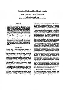
Fig. 1 Overview of our proposed framework. The training examples are provided to an anytime learner that can trade computation speed for better classifiers. The learning time, ρ l , can be preallocated (contract learning), or not (interruptible learning). Similarly, the maximal classification budget, ρ c , may be provided to the learner (pre-contract classification), provided to the classifier (contract classification), or be unknown (interruptible classification)

and thus must be prepared to be interrupted at any moment. While the assumption of preallocated resources holds for many induction tasks, in many other real-life applications it is not possible to allocate the resources in advance. By definition, every interruptible algorithm can serve as a contract algorithm because one can stop the interruptible algorithm when all the resources have been consumed. Russell and Zilberstein (1996) showed that the other direction works as well: any contract algorithm A can be converted into an interruptible algorithm B with a constant penalty. B is constructed by running A repeatedly with exponentially increasing time limits. One problem with this sequencing approach is the exponential growth of the gaps between the times at which an improved result can be obtained. Another problem is the use of the contract algorithm as a black box, disallowing the use of intermediate results. While we focus in this work on contract learners, we will discuss how the proposed contract algorithms can be made interruptible using iterative improvement techniques that address the shortcomings of the general sequencing approach. 2.2 Classification costs During classification, costs are associated with the measurements required by the model and with the prediction errors. Following previous works on cost-sensitive induction, we adopt the model described by Turney (1995). In a problem with |C| classes, a misclassification cost matrix M is a |C| × |C| matrix whose Mi,j entry defines the penalty of assigning the class ci to an instance that actually belongs to the class cj . Let "(H, e) be the set of tests required by a hypothesis H to classify a case e. We denote by cost(θ)!the cost of administering the test θ . The testing cost of e in H is therefore tcost(H, e) = θ∈" cost(θ). In addition, the model allows attributes that share a common cost to be part of a group. When the first test from the group is administered, we charge for the full cost. If another test from the same group is administered, we apply a group discount. The total cost of classification is the sum

Mach Learn (2011) 82: 445–473

449

of the miscalculation cost and the testing cost. Cost-sensitive classifiers, which aim to reduce the total cost of classification, require Mi,j and cost(θ) to be given in the same currency. Many environments, however, involve strict limits on the testing costs. To operate in such environments, the classifier needs to do its best without exceeding the bounds. Hence, classifiers that focus on reducing the total cost may be inappropriate. Like the bound on learning time, the bound on classification cost can be preallocated and given to the learner (pre-contract classification), provided only to the classifier (contract classification), or determined during classification (interruptible classification). 2.3 Anytime learning, anycost classification The allocation of resources for learning and for classification is driven by different factors. Therefore, our proposed framework needs to allow each allocation to be controlled independently. Moreover, the interruptibility of the learner is not necessarily tied to that of the classifier: an interruptible learner should be able, if required, to produce a contract classifier, and vice versa. Figure 1 gives an overview of the different possible scenarios for learning and classification. More formally, let E be the set of training examples, A be the set of attributes, along with their costs, and M be the misclassification cost matrix. Further, let ρ l be the allocation for learning resources and ρ c be the limit on classification resources for classifying a case e. For the scenarios where ρ l or ρ c are unknown, we assume two binary functions f l () and f c (), which can be queried by the learner and the classifier respectively to find out whether their resources have been exhausted. In this work we propose a novel framework that can be applied in the following constraint combinations: – Contract learning, pre-contract classification (CLPC): the learner is aware of both ρ l and ρ c . It produces a classifier that uses at most ρ c (the classifier does not benefit from any remaining surplus). Formally, CLPC(E, A, M, ρ l , ρ c ) → h(e). – Interruptible learning, pre-contract classification (ILPC): similar to CLPC but the learning time is not preallocated. Formally, ILPC(E, A, M, f l (), ρ c ) → h(e). – Contract learning, contract classification (CLCC): the learner is aware of ρ l but not of ρ c , which becomes available right before classification. The learner must produce a classifier that can operate under different cost constraints. The produced classifier should act according to the provided ρ c . Formally, CLCC(E, A, M, ρ l ) → h(e, ρ c ). – Interruptible learning, contract classification (ILCC): similar to CLCC but the learning time is not predetermined. Formally, ILCC(E, A, M, f l ()) → h(e, ρ c ). – Contract learning, interruptible classification (CLIC): the learner is aware of ρ l . Neither the learner nor the classifier is provided with ρ c . The learner must produce a classifier that utilizes the available resources until interrupted and queried for a solution. Formally, CLIC(E, A, M, ρ l ) → h(e, f c ()). – Interruptible learning, interruptible classification (ILIC): similar to CLIC but the learning time is unknown. Formally, ILIC(E, A, M, f l (), ρ c ) → h(e, f c ()). In each of the aforementioned scenarios, and unlike the cost-sensitive setup used by Turney (1995), we do not require Mi,j and ρ c to be provided in the same currency. This allows us to operate in environments where it is not possible to convert from one scale to another, for example time to money or money to risk. In the next section we present TATA, our proposed framework for anytime learning of anycost classifiers. TATA can operate under each of the aforementioned scenarios.

450

Mach Learn (2011) 82: 445–473

3 The TATA framework To act under the different cost scenarios presented in Sect. 2, we propose a framework into which any anytime pre-contract learner may be plugged. When configured to produce contract or interruptible classifiers, the framework builds a repertoire (committee) of precontract classifiers, each of which is designed to operate under a different classification budget. We start by motivating and describing our choice of tree-based pre-contract classifiers. We then introduce our anytime algorithm for learning pre-contract trees, and conclude by presenting our repertoire approach for contract and interruptible classification. 3.1 Tree-based pre-contract classifiers The pre-contract component should be able to control testing costs efficiently, and to exploit additional learning resources in order to improve the produced models. For the first requirement, a decision-tree based classifier would make an ideal candidate. When classifying a new case, decision trees ask only for the values of the tests on a single path from the root to one of the leaves. Decision tree models are also considered attractive due to their interpretability (Hastie et al. 2001), an important criterion for evaluating a classifier (Craven 1996), their simplicity of use, and their accuracy, which has been shown to be competitive with other classifiers for several learning tasks. Decision trees, however, cannot be used as is: when the classification budget does not allow exploring the entire path, the tree cannot make a decision. This problem can be overcome by storing a default class at each internal node. If classification is stopped early, the prediction is made according to the last explored node. Formally, let ρ c be the bound on testing costs for each case. When classifying an example e using a tree T , we propagate e down the tree along a single path from the root of T until a leaf is reached or classification resources are exhausted. Let "(T , e) be the set of tests along this path. We denote by cost(θ) ! the cost of administering the test θ . The testing cost of e in T is therefore tcost(T , e) = θ∈"(T ,e) cost(θ). Note that tests that appear several times are charged for only once. The cost of a tree is defined as the maximal cost of classifying an example using T . Formally,  0, T is a leaf Test-Cost(T ) = cost(θ ˆ ) + max Test-Cost( T ), otherwise. root(T )  Tˆ ∈ Children (T ) Having decided about the model, we are interested in a learning algorithm that can exploit additional time resources, preallocated or not, in order to improve the induced anycost trees. We recently presented two anytime algorithms for learning decision trees. The first, called LSID3 (Esmeir and Markovitch 2007b), can trade computation speed for smaller and more accurate trees, and the second, ACT, can exploit extra learning time to produce more cost-efficient trees. Neither algorithm, however, can produce trees that operate under given classification budgets; therefore, they are inappropriate for our task. 3.2 Anytime learning of pre-contract trees The most common method for learning decision trees is TDIDT (top-down induction of decision trees). TDIDT algorithms start with the entire set of training examples, partition it into subsets by testing the value of an attribute, and then recursively build subtrees. The TDIDT scheme, however, does not take into account bounds on the testing cost. Therefore, we first

Mach Learn (2011) 82: 445–473

451

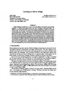
Fig. 2 Exemplifying the recursive invocation of TDIDT$. The initial ρ c was $60 (left-hand figure). Since two tests (a2 and a5 ) with a total cost of $30 have been used, their current cost is zero and the remaining budget for the TDIDT$ process is $30. a1 , whose cost is $40, is filtered out. Assume that, among the remaining candidates, a6 is chosen. The subtrees of the new split (right-hand figure) are built recursively with a budget of $20 Fig. 3 Top-down induction of anycost decision trees. E is the set of examples and A is the set of attributes

Procedure TDIDT$(E, A, ρ c ) If E = ∅ Or ρ c ≤ 0 Return Leaf(nil) If ∃c such that ∀e ∈ E class(e) = c Return Leaf(c) θ ← C HOOSE -T EST(A, E, ρ c ) V ← O UTCOMES(θ) Foreach vi ∈ V Ei ← {e ∈ E | θ (e) = vi } Si ← TDIDT$(Ei , A, ρ c − cost(θ)) Return Node(θ, {*vi , Si + | i = 1 . . . |V |})

describe TDIDT$, a modification for adapting any TDIDT algorithm to the pre-contract scenario. TDIDT$ filters out splits whose cost exceeds the remaining budget, and stops the recursive partitioning when additional splits cannot be afforded. We then consider the question of split selection in TDIDT$ algorithms, and introduce the pre-contract component in the TATA framework. 3.2.1 Top-down induction of anycost trees Traditional TDIDT algorithms do not consider limits on classification costs. Expensive tests, in this case, may block their subtrees and make them useless. In the pre-contract setup, ρ c , the maximal testing cost, is known in advance. Figure 3 formalizes our modified TDIDT procedure, denoted TDIDT$. TDIDT$ avoids exceeding ρ c by considering only tests whose costs are lower. When a choice is made to split on a test θ , the cost bound for building the subtree under it is decreased by cost(θ). Figure 2 exemplifies the recursive invocation of TDIDT$. The initial ρ c was $60 (left-hand figure). Since two tests (a2 and a5 ) with a total cost of $30 have been used, their current cost is zero and the remaining budget for the TDIDT$ process is $30. a1 , whose cost is $40, is filtered out. Assume that, among the remaining candidates, a6 is chosen. The subtrees of the new split (right-hand figure) are built recursively with a budget of $20.

452

Mach Learn (2011) 82: 445–473

TDIDT$ is designed to search in the space of trees whose test-cost is at most ρ c . It can be instantiated by means of an attribute selection procedure. 3.2.2 Greedy TDIDT$ instantiations Our first proposed anycost learner, called C4.5$, instantiates TDIDT$ by taking information gain as the split selection criterion, as in C4.5. Unlike the original C4.5, C4.5$ filters out unaffordable tests. It does not, however, consider the costs of the remaining candidates. Assume, for example, that the cost of the attribute with the highest information gain is exactly ρ c , the maximal classification budget. C4.5$ will choose to split on it and will not be able to further develop the tree. The EG2 algorithm (Nunez 1991) chooses attributes based on their Information Cost Function, ICF(θ) = (2$I (θ) − 1)/(cost(θ) + 1), where $I is the information gain. We denote by EG2$ an instantiation of TDIDT$ that uses ICF. EG2$ does not use ρ c when evaluating splits and therefore might over-penalize informative yet costly attributes, even when ρ c is large enough. This problem is intensified when the immediate information gain of relevant attributes is low, for example due to inter-correlation as in XOR-like concepts. 3.2.3 The pre-contract-TATA algorithm Both C4.5$ and EG2$ require a fixed short runtime and cannot exploit additional resources to improve the resulting classifier. Our recently introduced ACT algorithm overcomes the problems greedy cost-sensitive learners encounter by allowing learning time to be traded for lower total classification costs. ACT is an anytime TDIDT algorithm that invests more time resources for making better split decisions. For every candidate split, ACT attempts to estimate the total expected cost of using the resulting subtree were the split to take place. The estimation is based on a biased sample of the space of trees rooted at the evaluated attribute. The sample is obtained using a stochastic version of EG2, denoted Stochastic-EG2. ACT is a contract anytime algorithm parameterized by r, the number of trees in the sample.1 When r is larger, the resulting estimations are expected to be more accurate, improving the final tree. ACT attempts to minimize the sum of the testing and misclassification costs. However, it does not consider the maximal classification budget and may violate testing cost limits. Therefore, it is inappropriate for building pre-contract anycost classifiers. TATA, our proposed anytime learner, has a different goal: minimizing the misclassification costs given a bound on the testing costs. Hence, TATA must take a different approach for (1) top-down induction, (2) pruning, (3) biasing the sample, and (4) evaluating trees in the sample. While ACT adopts the TDIDT approach, in TATA we use TDIDT$. This carries 2 benefits: first, it guarantees that the produced tree will not violate the maximal cost, and second, it filters out some of the attributes and saves their evaluation time, which can be costly in the anytime setup. Once the tree is built, ACT post-prunes it in an attempt to reduce testing and misclassification costs. In TATA reducing testing costs is not beneficial because the built tree already fits the budget. Therefore, the objective of TATA’s post-pruning is to reduce misclassification costs, regardless of testing costs. When misclassification costs are uniform, this problem reduces to maximizing accuracy and thus we adopt C4.5’s error-based pruning (EBP). When misclassification cost is not uniform, we slightly modify EPB, and prune if the expected misclassification costs decrease (rather than the expected error). 1 As a contract algorithm, ACT assumes that the learning time is predetermined. Mapping contract time to r was discussed in a previous work (Esmeir and Markovitch 2007b).

Mach Learn (2011) 82: 445–473

453

Fig. 4 Attribute evaluation in Pre-contract-TATA. E-MC stands for the expected misclassification cost. For each candidate split, we sample the space of trees under it that fit the remaining budget ($60 in the example) and evaluate the split by the minimal expected misclassification cost in the sample ($110 in the example)

Procedure TATA-C HOOSE -ATTRIBUTE (E, A, r, ρ c ) If r = 0 Return C4.5$-C HOOSE -ATTRIBUTE(E, A, ρ c ) Foreach θ ∈ {θ ∈ A|cost(θ) < ρ c } V ← O UTCOMES(θ) Foreach vi ∈ V Ei ← {e ∈ E | θ (e) = vi } T ← C4.5$(Ei , A, ρ c − cost(θ)) mini ← E XPECTED MC(T ) Repeat r − 1 times T ← S TOCHASTIC -C4.5$(Ei , A, ρ c − cost(θ)) mini ← min(mini , E XPECTED MC(T )) ! | totalθ ← |V i=1 mini Return θ for which totalθ is minimal Fig. 5 Attribute selection in pre-contract-TATA. E XPECTED MC(T ) returns the expected misclassification cost of T

Like ACT, TATA samples the spaces of subtrees under each split to estimate its utility. ACT uses Stochastic-EG2 to bias the sample towards low-cost trees. In TATA, however, we would like to bias our sample towards accurate trees that fit our testing costs budget. Therefore, instead of using Stochastic-EG2, we designed a stochastic version of C4.5$, called Stochastic-C4.5$.2 In Stochastic-C4.5$ attributes are chosen semi-randomly, proportionally to their information gain. Note that the cost of the attributes affects the split decisions twice: first, TDIDT$ filters out the unaffordable tests, and second, the sampled trees themselves must fit the remaining budget, which penalizes expensive tests when the budget is relatively 2 Unlike the Stochastic-ID3 algorithm used in our previous work (Esmeir and Markovitch 2007b), Stochastic-

C4.5 and Stochastic-C4.5$ post-prune the induced trees.

454

Mach Learn (2011) 82: 445–473

low. We also tried to sample using stochastic versions of EG2 and DTMC. However, these cost-sensitive samplers did not yield any benefit and in some cases over-punished features with high costs. Having decided about the sampler, we need to decide how to evaluate the sampled trees. ACT favors trees whose expected total cost is lowest. In TATA all sampled trees fit the budget and therefore we choose to split on the attribute whose subtree is expected to have the lowest misclassification cost, as exemplified in Fig. 4. Figure 5 formalizes the split selection component in pre-contract-TATA. Pre-contractTATA is a contract anytime algorithm parameterized by r, the number of trees to sample. For a given set of examples and attributes, the runtime complexity of TATA grows linearly with r, just as it does in ACT (Esmeir and Markovitch 2007a). When we cannot afford sampling (r = 0), TATA builds the tree using C4.5$. r is predetermined according to the allocated resources. In Sect. 3.2.4 we discuss the interruptible learner, which does not assume preallocation of resources. 3.2.4 Interruptible learning of pre-contract classifiers The algorithm presented in Sect. 3.2.3 requires r, the number of trees in the sample, as a parameter. When the learning resources are not predetermined, we would like the learner to utilize extra time until interrupted. In a previous work we presented IIDT (Esmeir and Markovitch 2007b), a general framework for Interruptible Induction of Decision Trees, that need not be allocated resources a priori. IIDT starts with building a greedy tree. Then, it repeatedly selects a subtree whose reconstruction is expected to yield the highest marginal utility, and rebuilds the subtree with a doubled allocation of resources. This iterative improvement approach presents a tradeoff between short and long term benefit. Rebuilding subtrees in upper levels results in significant improvements but requires more resources. Choosing deeper nodes, on the other hand, allows more frequent, yet smaller improvements. IIDT allows us to control the tradeoff between efficient resource use and anytime performance flexibility, by setting a granularity parameter. Depending on the specific task, the user can guide IIDT to rebuild the entire tree at every iteration, or focus on smaller, deep subtrees. The same iterative improvement approach can be applied to convert pre-contract-TATA into an interruptible algorithm. The initial greedy tree would be built with C4.5$, and subtree reconstructions would be made using pre-contract-TATA. The marginal utility of constructing a tree would take into account both the expected misclassification cost of the tree and the expected resources required by the reconstruction process. The interruptible version of pre-contract-TATA allows the learning process to be interrupted at anytime. The resulting classifier, however, is pre-contract: it is designed to operate under the provided cost budget. In the following subsections we present algorithms for learning contract and interruptible classifiers. 3.3 Learning contract classifiers The pre-contract classification scenario assumes that ρ c , the bound on testing costs, is known to the learner. In many real-life scenarios, however, we do not know ρ c before building the model; we therefore require classifiers that either get ρ c as a parameter before proceeding with classification (contract classification) or can do their best until stopped and queried for a decision (interruptible classification). Note that TDIDT$-based algorithms cannot be used as is because ρ c is unavailable at the time of learning. Obviously, C4.5 and EG2 can be

Mach Learn (2011) 82: 445–473 Fig. 6 Classifying a case using repertoires in contract-TATA

455

Procedure C ONTRACT-TATA-C LASSIFY (B, e, ρ c ) c∗ ← max{c | c ≤ ρ c ∧ ∃T , *c, T + ∈ B} T ∗ ← T | *c∗ , T + ∈ B Return C LASSIFY(T ∗ , e)

Procedure C ONTRACT-TATA-U NIFORM -L EARN (E, A, r, k) c ← M INIMAL -ATTRIBUTE -C OST(A) ρmin c ← T OTAL -ATTRIBUTE -C OSTS(A) ρmax % i c c c C ← k−1 i=0 {ρmin + k−1 (ρmax − ρmin )} Return {*c, P RE - CONTRACT-TATA(E, A, r, c)+ | c ∈ C} Fig. 7 Building repertoires in contract-TATA with uniform cost gaps

slightly modified, by storing default classifications at each internal node to produce contract and interruptible trees; these algorithms do not need the value of ρ c . However, they are not designed to exploit a given testing budget. Therefore, we are looking for a learner that has the advantages of pre-contract-TATA without getting the value of ρ c as parameter. 3.3.1 Repertoire of trees Clearly, different classification budgets lead to different decision making strategies. When allocated a low budget, the contract classifier should rely on a small number of inexpensive tests. On the other hand, when the budget is high, the same classifier can afford to conduct expensive tests. Therefore, a good contract classifier must be prepared to utilize any ρ c it gets. For this purpose we suggest using pre-contract-TATA to build a collection of k trees, each with a different value of ρ c . We call such a collection a repertoire. In pre-contractTATA we exploit extra learning resources in order to increase r, the number of trees in the sample, and thus improve attribute-utility estimations. When composing a repertoire we can benefit from additional learning time either for building trees of higher quality or for increasing the granularity of the repertoire. The values of k and r impose a tradeoff between tree quality and granularity. Larger values of r mean better trees. Larger values of k mean less time to invest in each tree and higher memory requirements but increase the chances of finding a tree that fits the allocation. These chances depend also on the selection of ρ c c c values. Let ρmax be the cost of taking all tests and let ρmin be the cost of the least expensive c c or ρ c < ρmin . Therefore, attribute. Obviously, there is no need to build trees with ρ c > ρmax c c − ρmax ], where the difference in the we uniformly distribute the k values in the range [ρmin ρc

−ρ c

cost contract of each two successive trees is δ = mink−1max . Similarly to ensemble-based methods, a repertoire stores the k trees in memory. Therefore, its space complexity grows linearly with k. The runtime complexity also grows, on average, linearly with k.3 Figure 7 formalizes the procedures for forming repertoires with uniform gaps under the contract setup. Repertoires with nonuniform cost gaps are considered in Sect. 3.3.2.

3 Building trees for lower classification budgets takes, on average, less time, while building trees that can

exploit higher classification budgets takes, on average, more time.

456

Mach Learn (2011) 82: 445–473

Procedure C ONTRACT-TATA-H ILL -L EARN (E, A, r, k) c ← M INIMAL -ATTRIBUTE -C OST(A) ρmin c ← T OTAL -ATTRIBUTE -C OSTS(A) ρmax c ) Tmin ← P RE - CONTRACT-TATA(E, A, r, ρmin c ) Tmax ← P RE - CONTRACT-TATA(E, A, r, ρmax c c , Tmin +, *ρmax , Tmax ++ B ← **ρmin While |B| < k i ← arg maxi=1,...,|B|−1 (EE(Ti ) − EE(Ti+1 )) ∗ (ci+1 − ci+1 ) c +c c +c I NSERT-S ORTED(B, * i 2 i+1 , P RE - CONTRACT-TATA(E, A, r, i 2 i+1 )+) Return B Fig. 8 Building repertoires in contract-TATA using the hill-climbing approach

Unlike ensembles that combine predictions from several trees, the final decision of a repertoire classifier is based on a single tree. In the contract setup, classification resources are preallocated and therefore we pick a tree from the repertoire that best fits the cost bound. ρ c −ρ c Given a repertoire B and a classification budget ρ c , we would use the ( δ min + 1)th tree in the repertoire. However, a tree does not necessarily use the maximal cost it is allowed to use. Therefore when a tree is formed, we store it along with its actual maximal cost ρ&c . In the classification phase, we choose the tree associated with the largest c that does not exceed ρ&c . Figure 6 formalizes the procedures for using a repertoire to classify a case under the contract setup. 3.3.2 Learning repertoires with nonuniform cost gaps

In repertoires with uniform cost distribution, every two successive trees are built with maximal cost allocations that differ by δ. In many domains, however, increasing the contract by δ results in the same tree or a tree that performs similarly. In such a case, the efforts to build the second tree are wasted. These efforts could have been invested in more interesting cost regions where increasing the contract is useful. This problem is intensified when k, the repertoire size, is small. Consider, for example, a problem with 4 attributes, 3 of which c c = 1 and ρmax = 16. Assume that we cost $1 and 1 of which costs $13. In this case, ρmin would like to build a repertoire of size k = 4. Because δ = 5, the four trees will be built with ρ c = 1, 6, 11, 16 respectively. As a result, the 2nd and the 3rd trees would be identical because they can test the same set of attributes (all but the expensive one). Another problem with the uniform approach is the requirement that k, the repertoire size, be decided in advance. This is affordable when learning resources are predetermined (contract learning) but imposes a problem if the learning process itself needs to be interruptible. In Sect. 3.2.4 we described an interruptible version of the pre-contract learner, which produces a single tree and iteratively improves it. This technique, nevertheless, cannot be applied to build a repertoire of several trees. To overcome the aforementioned shortcomings, we propose a different approach for choosing the sequence of ρ c values in a repertoire. Rather than uniform gaps, we propose an iterative improvement solution. We start with a repertoire that consists of two trees: one c c and the other with ρmax . We then repeatedly choose two successive trees, built with ρmin T1 and T2 , built with ρ1c and ρ2c respectively, and add another tree with ρ c = 0.5(ρ1c + ρ2c ). Throughout the process, the stored trees are sorted by ρ c . Choosing ρ1c and ρ2c is not trivial. We are interested in maximizing the benefit from adding a new tree. Therefore, ρ2c − ρ1c should be large enough to cover a wide range of potential ρ c

Mach Learn (2011) 82: 445–473 Fig. 9 Using repertoires in interruptible-TATA

457

Procedure I NTERRUPTIBLE -C LASSIFY (&, e) While N OT-I NTERRUPTED T ← N EXT-T REE(&) l ← C LASSIFY(T , e) Return l

values. At the same time, the expected reduction in misclassification costs, if a tree is built in between, should be significant. To estimate the latter we use the expected errors of the built trees. Two successive trees whose expected errors vary significantly indicate that it may be worthwhile to build a tree in between them. Combining these two criteria, we choose T1 and T2 that maximize (ρ2c − ρ1c ) · (EE(T2 ) − EE(T1 )). In this case, setting ρ c of the new tree to 0.5(ρ1c + ρ2c ) is optimal. We refer to this method as a hill-climbing repertoire. This process can be repeated until the learner is interrupted, or until a predetermined number of trees have been built. Figure 8 formalizes the procedure for building hill-climbing repertoires. Similarly to the uniform-gaps case, each tree is stored along with its actual maximal classification cost. When classifying an instance, we choose the tree that best fits the given classification limit. 3.4 Learning interruptible classifiers In the interruptible setup, the classification budget is provided neither to the learner nor the classifier. The classifier is expected to utilize resources until it is interrupted and queried for class label. To operate in such a setup, we again form repertoires. Unlike the contract setup, however, ρ c is available to the classifier. Therefore, we cannot choose a single tree for classification. We first describe the use of repertoires for interruptible classification, and then address the problems that may arise when traversing multiple trees. 3.4.1 Forming repertoires for interruptible classification One solution is to form a repertoire with uniform gaps, similarly to the contract setup (see Fig. 7). When we need to classify an instance, we start by using the lowest-cost tree, which c . We then move on to the next tree, as long as resources allow. When is built with ρ c = ρmin interrupted, we use the prediction of the last fully explored tree as the final decision. Since the trees in the repertoire are sorted by their ρ c , the last fully explored tree is expected to have better predictability than those preceding it.4 Figure 9 formalizes the classification procedure under the interruptible setup. While simple, this approach raises two important considerations. First, because we are charged for the cumulative cost of using the trees, it is no longer ideal to have as many trees in the repertoire as possible. Second, when forming the repertoire, the learner should take into account tests that appear in previous trees in the repertoire because their outcome might have been already known when using the tree for classification. 3.4.2 Determining the size of interruptible repertoires Determining the repertoire size is not trivial. Even if we are not limited in our learning resources, we would like to limit the number of trees in the repertoire to avoid wasting 4 Instead of relying solely on the last tree, a weighted voting decision can be made. However, in this work we

chose to focus on single-tree decisions, which allow better interpretability.

458

Mach Learn (2011) 82: 445–473

Fig. 10 An example of applying cost discounts when forming a repertoire for interruptible classification. The numbers represent the number of examples that follow each edge. Because the value of a1 is required at the root of T1 , any subsequent tree can obtain this value at no cost. The probability for testing a2 is 50% in T2 . When inducing T3 , the attribute a2 has already been measured with a probability of 50%. Hence, we discount the cost of a2 by 50% ($5 instead of $10). Similarly, the cost of a3 is discounted by 80% ($2 instead of $10)

classification resources on trees that will not affect the final decision. On the other hand, if the repertoires are too small, it might not be possible to optimally exploit the available classification resources. Obviously, the optimal size depends much on the characteristics of the problem. In our experimental study we will consider using a fixed number of trees. In the future, we intend to analyze this problem theoretically and find the optimal value. This task is even more challenging because of the second issue (re-administering tests). 3.4.3 Discounting repeated tests Once a tree is used for classification and the relevant tests in the decision path are administered, we do not charge for the same test in the subsequent trees because its outcome is already at hand. The learner could use this information to improve the structure of the repertoire. Assume, for example, that the value of an attribute a1 is measured at the root node of the first tree in the repertoire. Subsequent trees that ask for a1 ’s value are not charged. Therefore, when building the subsequent trees, the cost of a1 should be treated as zero. Nevertheless, given a case to classify, not all tests that appear in earlier trees are necessarily administered, but only those that appear in decision paths that have been followed. Obviously, one cannot know in advance which tree paths will be followed because this depends on the feature values of the actual case. To handle this situation we take a probabilistic approach. We assume that future test cases will come from the same distribution as the training examples. Let T1 , . . . , Ti be the trees that have already been built. When building Ti+1 , we discount the cost of each attribute by the probability of examining its value at least once in T1 , . . . , Ti . For an attribute a, we measure this probability by the percentage of training examples whose a value would have been queried by previous trees. Consider, for example, the trees in Fig. 10. The probability to measure a1 in T1 is 100%. Therefore, when building subsequent trees, the cost of a1 would be zero. The probability for testing a2 is in T2 20%. Hence, when inducing T3 , we discount the cost of a2 by 20% ($8 instead of $10). Similarly, the cost of a3 is discounted by 80% ($2 instead of $10). Because the trees may be strongly correlated, we cannot simply calculate this probability independently for each tree. For example, if T3 in the aforementioned example tests a2 for 70% of the examples, we would like to know for how many of these examples a2 has been tested also in T2 . Therefore, we traverse the previous trees with each of the training examples and mark the attributes that are tested at least once. For efficiency, the matrix that

Mach Learn (2011) 82: 445–473

459

Procedure A PPLY-D ISCOUNT (E, A, &) Mi,j ← 0 Foreach e ∈ E Foreach T ∈ & Aˆ ← attributes whose values tested by T when classifying e Foreach a ∈ A Me,a ← 1 Foreach a ∈ Aˆ !|E|

M

a,e pa ← e=1 |E| cost(a) ← cost(a) · (1 − pa )

Fig. 11 Procedure for applying discounts when forming discount repertoires for interruptible classification

Fig. 12 The different components of the TATA framework. Pre-contract-TATA (top) is provided with ρ c , and produces a classifier that operates within that bound. Contract-TATA (left) and Interruptible-TATA (right) build a repertoire of pre-contract classifiers, learned using pre-contract-TATA. The classifiers are ordered by ρ c (lowest first). In the case of contract classification, a single classifier (grayed) is chosen to classify each instance. In the case of interruptible classification, the classifiers are explored while resources permit (grayed). The last result obtained before interruption is returned

represents which tests were administered for which case is built incrementally and updated after building each new tree. We refer to this method as a discount repertoire. The repertoire is formed using the same method in Fig. 7 with a single change: before building each tree, cost discounts are applied; the discounts are based on the trees already in the repertoire. Figure 11 formalizes the procedure for updating test costs. During classification we iterate over the trees until interrupted, as described in Fig. 9. 3.5 The TATA framework components: a summary We presented three different components of TATA for the three different classification cost scenarios. Pre-contract-TATA allows learning decision trees that can operate under a predetermined classification budget. Contract-TATA builds a repertoire of pre-contract trees, each

460 Table 1 Comparing MC, the misclassification cost, for different testing cost contracts. The numbers represent the average over 100 datasets. The last column indicates whether the advantage of TATA(r = 5) is statistically significant according to the Wilcoxon test (α = 5%)

Mach Learn (2011) 82: 445–473 Learner TATA(r = 5) C4.5

TATA(r = 0)

c ' ρmax

1 ρc 3 max

MC(ρ c )

21.12 28.84 26.93

EG2

31.21

EG2$

30.48

Wilcoxon

√

√ √ √

with a different classification budget. When classifying a new case, the classifier picks the tree that best suits the available resources and uses it for classification. Similar to contractTATA, interruptible-TATA builds a repertoire of pre-contract trees. During classification, however, it explores the trees in the repertoire in order (lowest classification cost first). When interrupted, it returns the decision made by the last fully explored tree. While both contractTATA and interruptible-TATA use pre-contract-TATA to build repertoires, their consideration of repertoire size and tree budgets differ due to the difference in the way the classifiers are used. For each of the three components, we presented a contract anytime learner and discussed what steps to take when learning needs to be interruptible. Figure 12 summarizes the interconnection between TATA’s components. While in this work we focused on tree-based classifiers, any pre-contract classifier can be plugged in TATA to produce contract and interruptible classifiers. 4 Experimental evaluation A variety of experiments were conducted to test the performance and behavior of TATA in 3 different setups: pre-contract, contract, and interruptible. Recently, we presented an automatic method for assigning testing costs to attributes in existing datasets (Esmeir and Markovitch 2007a). We applied this method 4 times on 20 UCI (Asuncion and Newman 2007) problems5 and another 5 datasets that hide hard concepts and have been used in previous machine learning literature. Appendix gives a detailed description of these datasets.6 Following the recommendations of Bouckaert (2003), 10 runs of a 10-fold crossvalidation experiment were conducted for each dataset and the reported results are averaged over the 100 individual runs. This setup allows relatively higher replicability of the results. 4.1 Pre-contract classification We first compare pre-contract TATA to several other pre-contract learners, and then we examine TATA’s anytime behavior. 4.1.1 Comparison under different budgets Our first set of experiments compares C4.5, EG2, EG2$, TATA(r = 0), which is equivalent to C4.5$, and TATA(r = 5), which samples 5 trees at each node to choose a split, in the precontract setup. Misclassification has been set uniformly to 100. Note that the absolute value 5 The datasets vary in size, type of attributes, and dimension. 6 The 4 × 25 datasets are available at http://www.cs.technion.ac.il/~esaher/publications/rbc.

Mach Learn (2011) 82: 445–473

461

Fig. 13 Pre-contract results: the misclassification cost for different preallocated testing costs, as percentage of the total cost. The results are averaged over all 100 datasets

of the misclassification cost does not matter because we do not assume same-scale. ACT, ICET, and DTMC cannot be applied in such a setup because they require the tradeoff factor between misclassification cost and testing cost to be given. This is one of the important differences between TATA and cost-sensitive learners that attempt to minimize the total cost of classification. For each dataset we invoked the algorithms 30 times, each with a different ρ c value taken c ), with uniform steps. Figure 13 describes the misclassification from the range [0, 120%ρmax cost of the different algorithms, as a function of ρ c . For each point (ρ c value), the results are averaged over the 100 datasets. c , the algorithms cannot administer Clearly, TATA(r = 5) is dominant. When ρ c ≤ ρmin c , the atany test and thus their performance is identical. At the other end, when ρ c ≥ ρmax tribute costs are actually not a constraint. In this case TATA(r = 5) performed best, confirming the results reported in Esmeir and Markovitch (2007a) when misclassification costs were dominant. The more interesting ρ c values are those in between. Table 1 lists the normalized c c , ρmax ]. Confirming the area under the misclassification cost curve over the range [ 13 ρmax curves, the results indicate that TATA(r = 5) has the best overall performance. The Wilcoxon test (Demsar 2006), which compares classifiers over multiple datasets, finds TATA(r = 5) to be significantly better than all the other algorithms. As expected, all five algorithms improve with the increase in ρ c because they can use c , we can see that EG2, which is costmore features. For ρ c values slightly larger than ρmin sensitive, performs better than C4.5. The reason is that EG2 takes into account attribute costs and hence will prefer lower cost attributes. With the increase in ρ c and the relaxation of cost constraints, C4.5 becomes better than EG2. It is interesting to compare the TDIDT$ variants of C4.5 and EG2 to their TDIDT counterparts. It is easy to see that both TDIDT$ variants exhibit better anycost behavior, until the c ), where the performance of each point where all relevant attributes can be used (ρ c ∼ ρmax pair becomes identical. The advantage of the TDIDT$ variants is due to their not choosing tests that violate the cost limits; thus, they will not be forced to stop the classification process earlier. A comparison of TATA(r = 0) to TATA(r = 5) indicates that the latter is clearly better: while TATA(r = 0) chooses split attributes greedily, TATA(r = 5) samples the possible subtrees of each candidate and bases its decision on the quality of the sampled trees. Of course, the advantage of TATA(r = 5) comes at a price: it uses far more learning resources.

462

Mach Learn (2011) 82: 445–473

Fig. 14 Pre-contract results: the misclassification cost as a function of the preallocated testing costs contract for one instance of Glass (upper-left), AND-OR (upper-right), MULTI-XOR (lower-left) and KRK (lower-right)

Figure 14 gives the results for 4 individual datasets, Glass, AND-OR, MULTI-XOR and KRK. In all 4 cases TATA is dominant with its r = 5 version being the best method. We can see that the misclassification cost decreases almost monotonically. The curves, however, are less smooth than the average result from Fig. 13 and slight degradations are observed. The reason could be that irrelevant features become available and mislead the learner. The KRK curve looks much like steps. The algorithms improve at certain points. These points represent the budgets when the use of another relevant attribute becomes possible. The graphs of AND-OR and MULTI-XOR do not share this phenomenon because these concepts hide interdependency between the attributes. As a result, an attribute may be useless if other attributes cannot be considered. The performance of the greedy C4.5 and TATA(r = 0) on these problems is very poor. 4.1.2 Anytime behavior of pre-contract TATA Besides being able to produce good anycost trees, TATA itself is an anytime algorithm that can trade learning resources for producing better trees. Our next experiment examines the anytime behavior of TATA by invoking it with different values of r. Figure 15 shows the results. As we can see, all TATA versions are better than C4.5. With the increase in r (larger samples of trees), the advantage of TATA increases. The most significant improvement is from r = 0 to r = 1. TATA with r = 0 is a greedy algorithm that uses local heuristics. When r > 0, TATA uses sampling techniques to evaluate attributes and thus improves notably. For more difficult concepts, where only a combination of a large number of attributes yields information, a larger value of r would be needed.

Mach Learn (2011) 82: 445–473

463

Fig. 15 TATA with different sample sizes on the Multi-XOR dataset

Fig. 16 Contract results: the misclassification cost as a function of the preallocated testing costs contract for Glass (upper-left), AND-OR (upper-right), MULTI-XOR (lower-left) and KRK (lower-right)

4.2 Contract classification TATA uses repertoires to operate in the contract and interruptible setups. To examine the anycost behavior of TATA in the contract setup we built 3 repertoires, each of size 16. The first repertoire uses pre-contract-TATA(r = 0) to induce the trees, with uniform contract gaps. The second repertoire uses pre-contractTATA(r = 3) to induce the trees, with uniform contract gaps. The trees in the third repertoire are also formed using pre-contract-TATA(r = 3), but with the hill-climbing approach instead of uniform gaps.

464

Mach Learn (2011) 82: 445–473

Fig. 17 Learning repertoires with different time allocations and sample sizes. Each curve represents the normalized AUC for a fixed-time allocation and varying r values

The repertoires were used to classify examples in the contract setup. 120 uniformly disc ] were used as contract parameters. Figure 16 tributed ρ values in the range [0–120%ρmax describes the performance of these three repertoires on 4 datasets (Glass, AND-OR, MULTIXOR, and KRK), averaged over the 100 runs of 10 times 10-fold cross-validation. In addition, we report the results of the cost-insensitive C4.5. It is easy to see that across all 4 domains Uniform- and Hill-TATA(r = 3) are dominant. Uniform-TATA(r = 0) is better than C4.5 when the provided contracts are low. When the contracts can afford to use all the attributes, both algorithms perform similarly. In comparison to Uniform-TATA(r = 0), the anycost behavior of Uniform-TATA(r = 3) is better: it is monotonic and utilizes testing resources better. Uniform- and Hill-TATA(r = 3) exhibit interesting performance differences. While both algorithms display similar trends, Hill-TATA reaches better results slightly earlier than Uniform-TATA on 3 out of the 4 domains (with the exception of KRK). The reason is that Hill-TATA selects the series of ρ c ’s heuristically, rather than by means of blind uniform gaps. As a result, it can focus on cost ranges where it is worthwhile to build more trees. These differences are expected to diminish when the repertoires are larger, which enables Uniform-TATA to cover more contracts. To verify this hypothesis, we repeated the experiments with k = 32 and indeed the performance gap closed. It is important to note, however, that while Uniform-TATA is a contract learner that requires k in advance, Hill-TATA is an interruptible learner and is therefore appropriate also for cases where the learning resources are not preallocated. In Sect. 4.1 we examined the anytime behavior of the learner in the pre-contract setup. The results indicate that the misclassification costs decrease with the increase in the sample size (and hence learning resources). In the contract setup, given a fixed learning time, increasing the sample size comes at a price: reducing the number of trees in the repertoire. An interesting question is whether one should invest more resources in building better single trees or in forming larger repertoires. To investigate this, we learned several repertoires using the hill-climbing approach. The trees of each repertoire were induced with a different r parameter for pre-contract-TATA, from 0 up to 7. When r = 0, pre-contract-TATA behaves like the greedy C4.5$. In this case we assumed that an infinite number of trees can be built (in practice a tree was built for every tested value of ρ c ). Because we used the hill-climbing approach, we could stop the learning process at any time. We chose three different stopping points: 1 minutes, 3 minutes, and 5 minutes. We tested the performance of these 8 × 3 repertoires. Figure 17 gives the results. Each curve

Mach Learn (2011) 82: 445–473

465

Fig. 18 Results for interruptible classification: the misclassification cost as a function of the interruption costs for Glass (upper-left), AND-OR (upper-right), MULTI-XOR (lower-left) and KRK (lower-right)

stands for a different time allocation. The first plot gives the normalized AUC in the range c . ρ = 33%–99%ρmax It is easy to see that in all three graphs, increasing the learning time allows the production of more trees: the curve for T = 5 is lower than that of T = 3 and T = 1. Interestingly, for each of the fixed-time curves, a U shape is observed. On the one hand, if the samples are too small, it might be difficult to learn the concept perfectly. On the other hand, increasing r means more time per tree and thus results in smaller repertoires, without covering significant ranges of ρ c . In the extreme case, for example T = 1, r > 3, it is impossible to build even a single tree and the error-rate is 50%, as is the base-line error. We can see that the optimal value of r differs from one time allocation to another. 4.3 Interruptible classification In the interruptible classification setup, TATA forms a repertoire of trees and traverses it until interrupted. Unlike the contract setup, here we would like to limit the number of trees in the repertoire to avoid wasting resources on tests that will not be needed by the tree that makes the final decision. This would be the case even if we had infinite learning resources. However, too small repertoires may lead to poor performance in significant ρ c ranges. To examine the anycost behavior of TATA in the interruptible setup, we built three different repertoires: – Repertoire of 3 TATA(r = 0) trees with uniform distribution learned with attribute discounts. – Repertoire of 3 TATA(r = 3) trees with uniform distribution learned with attribute discounts.

466

Mach Learn (2011) 82: 445–473

– Repertoire of 16 TATA(r = 3) trees with uniform distribution learned with attribute discounts. The repertoires were used to classify examples in the interruptible setup. In addition, we c ] report the results of C4.5. 120 uniformly distributed ρ c values in the range [0–120%ρmax were used as interruption triggers. Figure 18 describes the performance of these repertoires on 4 datasets (Glass, AND-OR, MULTI-XOR, and KRK), averaged over the 100 runs of 10 times 10-fold cross-validation. As we can see, TATA(r = 3) variants achieve the best performance along a wide range of ρ c values. Interestingly, for some cases (e.g., MULTI-ANDOR) it is better to form smaller repertoires while for other cases (e.g., Glass) larger repertoires yield better results. Furthermore, in the MULTI-XOR problem k = 16 is better at the beginning, then at some point k = 3 becomes better, and finally they become almost equal. The reason for this phenomenon is that the k = 3 repertoire does not contain trees suitable for lower ρ c values. The k = 16 repertoire, on the other hand, spends too many resources on cheap trees, and hence its performance when ρ c increases is weaker than k = 3. At some point, however, both reach the same performance because they have administered all the relevant tests. An interruptible classifier can, by definition, operate under the pre-contract and contract classification settings. It cannot, however, exploit the additional information available in these setups, and therefore might underperform. The results reported for pre-contract-TATA and interruptible-TATA show that when the classification budget is known to the learner, precontract-TATA is clearly the best choice. For example, in the MULTI-XOR problem, precontract-TATA reaches its optimal results for ρ c < 250 (Fig. 14), while interruptible-TATA has a higher misclassification cost even with ρ c = 300 (Fig. 18). Moreover, the learning resources used by pre-contract-TATA to build a single tree that fits the known budget are far less than those needed to build a repertoire. 5 Related work While, to the best of our knowledge, no specific attempt has been made to design an anytime algorithm for learning anycost decision trees, several related works, aside from those mentioned in the previous sections, warrant discussion here. Yang et al. (2007) introduced Anytime Averaged Probabilistic Estimators (AAPE) for utilizing additional computational resources during classification. At classification time, AAPE computes Naive Bayes and then exploits extra time to refine the probability estimate. Ueno et al. (2006) showed how to convert nearest neighbor classifiers into anytime classifiers. The proposed algorithm, called Anytime Nearest Neighbor (ANN), utilizes additional classification time by considering more and more examples out of which the nearest neighbor is picked. Unlike TATA, both AAPE and ANN are fixed-time learners and cannot benefit from additional resources during learning. Moreover, ANN and AAPE do not deal with attribute costs and assume that the major constraint is the computation time required by the probabilistic models. Cost-sensitive trees have been the subject of many research efforts. Several works proposed greedy learners that take into account test costs by modifying the split criteria; these include EG2 (Nunez 1991), IDX (Norton 1989), and CS-ID3 (Tan and Schlimmer 1989). These methods, however, do not consider misclassification costs. Other researchers introduced learning algorithms that consider different misclassification costs (Breiman et al. 1984; Pazzani et al. 1994; Provost and Buchanan 1995; Webb 1996; Bradford et al. 1998; Domingos 1999; Drummond and Holte 2000; Elkan 2001; Zadrozny et al. 2003;

Mach Learn (2011) 82: 445–473

467

Lachiche and Flach 2003; Abe et al. 2004; Vadera 2005; Margineantu 2005; Zhu et al. 2007; Sheng and Ling 2007b; O’Brien et al. 2008; Bourke et al. 2008). These methods, however, do not consider test costs and hence are appropriate mainly for domains where test costs are not a constraint. Recently, several research efforts have been invested in developing tree-learners that consider both test costs and misclassification costs, and look for a tree that minimizes their sum. In DTMC (Decision Trees with Minimal Cost), a greedy method that attempts to minimize both types of costs simultaneously, a tree is built top-down, and a greedy split criterion that takes into account both testing and misclassification costs is used (Ling et al. 2004; Sheng et al. 2006). The ICET algorithm (Inexpensive Classification with Expensive Tests, Turney 1995) was a pioneer in non-greedy search for a tree that minimizes test and misclassification costs. ICET uses genetic search to produce a new set of costs that reflects both the original costs and the misclassification cost reduction contributed by each attribute. Then it builds a tree using the EG2 algorithm but with the evolved costs instead of the original ones. Bayer-Zubek and Dietterich (2005) formulated the cost-sensitive learning problem as a Markov Decision Process (MDP), and used a systematic search algorithm based on the AO* heuristic search procedure to solve the MDP. Fan et al. (2000) studied the problem of cost-sensitive intrusion detection systems (IDS), where the goal is to maximize security while minimizing costs. Freitas et al. (2007) presented a greedy algorithm for decision tree induction that considers misclassification costs, testing costs, delayed costs, and costs associated with risk, and applied on several medical tasks. These methods, however, are not designed to produce anycost trees that can utilize strict classification budgets. Greiner et al. analyzed the theoretical aspects of learning cost-sensitive active classifiers using a variant of the probably-approximately-correct (PAC) model. They showed that is it possible to PAC-learn optimal trees that administer at most a predetermined constant number of tests. Their proposed method, however, requires O(nd ) time to find the optimal d-depth tree over n attributes. Farhangfar et al. (2008) presented a fast way to produce near-optimal depth-bounded trees under the Naive Bayes assumption. The proposed approach resulted in a speedup of O(n/ log n) and, despite the unrealistic assumption, it yielded relatively high classification accuracy. Even after this improvement, however, the algorithm is still exponential in d, the depth of the tree, and therefore impractical for problems with large n and d. Costs are also involved in the learning phase, during example acquisition. The problem of budgeted learning has been studied by Lizotte et al. (2003). There is a cost associated with obtaining each attribute value of a training example, and the task is to determine which attributes of which instances to test given a budget. Kun et al. (2007) presented algorithms based on the multi-armed bandit problem to operate in the budgeted learning setup. In a related work, Kaplan et al. (2005) explored the theoretical aspects of learning from data where observing the value of an attribute has an associated cost. An extension to the work on optimal bounded active classifiers (Greiner et al. 2002) is when tests have costs also during the learning phase. Kapoor and Greiner (2005) presented a budgeted learning framework that operates under strict budget for feature-value acquisition during learning and produces a classifier with a limited classification budget. Provost et al. (2007) discussed the challenges electronic commerce environments bring to data acquisition during learning and classification. They discussed several settings and presented a unified framework to integrate acquisition of different types, with any cost structure and any predictive modeling objective. A related problem is active feature-value acquisition. In this setup one tries to reduce the cost of improving accuracy by identifying highly informative instances. Melville et al.

468

Mach Learn (2011) 82: 445–473

(2004) introduced an approach in which instances are selected for acquisition using the accuracy of the current model and its confidence in the prediction. Our setup assumed that we are charged for acquiring each of the feature values of the test cases. The term test strategy (Sheng et al. 2005) describes the process of feature value acquisition: which values to query for and in what order. Several test strategies have been studied, including sequential, single batch and multiple batch (Sheng et al. 2006), each of which corresponds to a different diagnostic policy. These strategies are orthogonal to our work because they assume a given decision tree. Bilgic and Getoor (2007) tackled the problem of feature subset selection when costs are involved. The objective is to minimize the sum of the information acquisition cost and the misclassification cost. Unlike greedy approaches that compute the value of features one at a time, they used a novel data structure called the value of information lattice (VOILA), which exploits dependencies between missing features and makes it possible to share information value computations between different feature subsets. VOILA was shown empirically to achieve dramatic cost improvements without the prohibitive computational costs of comprehensive search. Nijssen and Fromont (2007) presented DL8, an exact algorithm for finding a decision tree that optimizes a ranking function under size, depth, accuracy and leaf constraints. The key idea behind DL8 is that constraints on decision trees are simulated as constraints on itemsets. They show that optimal decision trees can be extracted from lattices of itemsets in linear time. The applicability of DL8, however, is limited by two factors: the number of itemsets that need to be stored, and the time that it takes to compute these itemsets. In some cases, the number of frequent itemsets is so large that it is impossible to compute or store them within reasonable time or space.

6 Conclusions Machine learning techniques are increasingly popular in applications that involve constraints on classification budget, including, among others, hardware fault detection (Wang 2010), medical diagnosis (Kononenko 2001), spam detection (Dredze et al. 2007), network traffic (Kim et al. 2004; Wang and Yu 2009), and intra-day trading (Luss and d’Aspremont 2009). In this work we described three different scenarios for anycost classification. In the precontract setup the maximal cost is known to the learner; in the contract setup it is known after building the predictive model but before proceeding with classification; and in the interruptible setup the cost limit is provided neither to the learner nor the classifier. The major contribution of this paper is the TATA framework, which is designed to operate in such environments. For the pre-contract setup, TATA builds a tree top-down and exploits extra resources to make better split decisions. During the recursive induction, TATA considers only tests that fit the budget. For each split, it samples the space of subtrees under it that fit the remaining budget, and prefers the split under which there is a subtree with a minimal expected misclassification cost. For the contract and interruptible scenarios, TATA builds a repertoire of trees from several invocations of pre-contract-TATA with different cost limits. While in contract-TATA the tree that best fits the budget is picked, in interruptible-TATA the trees in the repertoire are traversed sequentially until interrupted, and the prediction of the last fully explored tree is returned. A great advantage of the repertoire concept is its generality: it can be easily configured to use any base classifier given a pre-contract learning algorithm for that classifier.

Mach Learn (2011) 82: 445–473

469

While our interruptible classifier can operate also under the pre-contract and contract classification setup, it comes at a price. First, during learning, resources are allocated for building trees that are eventually ignored. Unlike the pre-contract learner that invests 100% of the available learning time in a single tree, learners of contract and interruptible classifiers split their resources among several trees. Building 10 trees of the same quality as the precontract learner takes, on average, 10 times longer. Second, during classification, resources are wasted on testing attributes that may not affect the final decision. Unlike pre-contract and contract classifiers, which test only the attributes along a single path of a single tree, interruptible classifiers measure features from several trees. Some of these features may not be needed by the last fully explored tree. The learning components of TATA are themselves anytime, and can utilize extra learning resources to produce better anycost classifiers. These resources may be preallocated (contract learning) or not (interruptible learning). In the pre-contract setup, the TATA learner can utilize extra time to form larger samples and thus improve tree-utility estimations. In the contract and interruptible scenarios, extra time can be invested either to create better single trees or to enlarge the repertoires. The experimental study shows that TATA exhibits good anytime behavior and produces substantially better anycost classifiers. For many real-life problems that involve limits on testing cost, TATA makes it possible to obtain affordable decision trees with notably lower misclassification costs. Depending on the specific needs of the application, the user can choose to provide TATA with the classification budget either before learning the model, or before classifying each case. Alternatively, if the budget is not predetermined, the user can interrupt the classifier when the budget is exhausted without explicitly providing an upper bound. In the future we intend to examine other methods for producing the TATA samples. In addition, we plan to further research the tradeoff between the size of a repertoire and the quality of the trees composing it, both in the contract and interruptible setups.

Appendix: Datasets Table 2 lists the characteristics of the 25 datasets we used. Below we give a more detailed description of the non-UCI datasets used in our experiments: 1. Multiplexer: The multiplexer task was used by several researchers for evaluating classifiers (e.g., Quinlan 1993). An instance is a series of bits of length a + 2a , where a is a positive integer. The first a bits represent an index into the remaining bits and the label of the instance is the value of the indexed bit. In our experiments we considered the 20-Multiplexer (a = 4). The dataset contains 500 randomly drawn instances. 2. Boolean XOR: Parity-like functions are known to be problematic for many learning algorithms. However, they naturally arise in real-world data, such as the Drosophila survival concept (Page and Ray 2003). We considered XOR of five variables with five additional irrelevant attributes. 3. Numeric XOR: A XOR based numeric dataset that has been used to evaluate learning algorithms (e.g., Baram et al. 2003). Each example consists of values for x and y coordinates. The example is labeled 1 if the product of x and y is positive, and −1 otherwise. We generalized this domain for three dimensions and added irrelevant variables to make the concept harder.

470

Mach Learn (2011) 82: 445–473

Table 2 Characteristics of the datasets used Dataset

Instances

Attributes Nominal (binary)

Max att. Numeric

Domain

Classes

Breast Cancer

277

9 (3)

0

13

Bupa

345

0 (0)

5

–

2

Car

1728

6 (0)

0

4

4

Flare

323

10 (5)

0

7

4

Glass

214

0 (0)

9

–

7

Heart

296

8 (4)

5

4

2

Hepatitis

154

13 (13)

6

2

2

Iris

150

0 (0)

4

–

3

KRK

28056

6 (0)

0

8

17

Monks-1

124 + 432

6 (2)

0

4

2

6 (2)

0

4

2

122 + 432

6 (2)

0

4

2

20 (20)

0

2

2

Monks-2 Monks-3 Multiplexer-20

169 + 432 615

2

Multi-XOR

200

11 (11)

0

2

2

Multi-AND-OR

200

11 (11)

0

2

2

Nursery

8703

8 (8)

0

5

5

Pima

768

0 (0)

8

–

2

TAE

151

4 (1)

1

26

3

Tic-Tac-Toe

958

9 (0)

0

3

2

Titanic

2201

3 (2)

0

4

2

Thyroid

3772

15 (15)

5

2

3

Voting

232

16 (16)

0

2

2

Wine

178

0 (0)

13

–

3

XOR 3D

200

0 (0)

6

–

2

XOR-5

200

10 (10)

0

2

2

4. Multi-XOR/Multi-AND-OR: These concepts are defined over 11 binary attributes. In both cases the target concept is composed of several subconcepts, where the first two attributes determines which of them is considered. The other 10 attributes are used to form the subconcepts. In the Multi-XOR dataset, each subconcept is an XOR, and in the MultiAND-OR dataset, each subconcept is either AND or OR.

References Abe, N., Zadrozny, B., & Langford, J. (2004). An iterative method for multi-class cost-sensitive learning. In Proceedings of the 10th ACM SIGKDD international conference on knowledge discovery and data mining (KDD-2004), Seattle, WA, USA (pp. 3–11). Asuncion, A., & Newman, D. (2007). UCI machine learning repository. University of California, Irvine, School of Information and Computer Sciences. http://www.ics.uci.edu/~mlearn/MLRepository.html. Baram, Y., El-Yaniv, R., & Luz, K. (2003). Online choice of active learning algorithms. In Proceedings of the 20th international conference on machine learning (ICML-2003), Washington, DC, USA (pp. 19–26). Bayer-Zubek, V., & Dietterich, T.G. (2005). Integrating learning from examples into the search for diagnostic policies. Artificial Intelligence, 24(1), 263–303.

Mach Learn (2011) 82: 445–473

471

Bilgic, M., & Getoor, L. (2007). Voila: Efficient feature-value acquisition for classification. In Proceedings of the 22nd national conference on artificial intelligence (AAAI-2007), Vancouver, British Columbia, Canada (pp. 1225–1230). Boddy, M., & Dean, T. L. (1994). Deliberation scheduling for problem solving in time-constrained environments. Artificial Intelligence, 67(2), 245–285. Bouckaert, R. R. (2003). Choosing between two learning algorithms based on calibrated tests. In Proceedings of the 20th international conference on machine learning (ICML-2003), Washington, DC, USA (pp. 51– 58). Bourke, C., Deng, K., Scott, S. D., Schapire, R. E., & Vinodchandran, N. V. (2008). On reoptimizing multiclass classifiers. Machine Learning, 71(2–3), 219–242. Bradford, J., Kunz, C., Kohavi, R., Brunk, C., & Brodley, C. (1998). Pruning decision trees with misclassification costs. In Proceedings of the 9th European conference on machine learning (ECML-1998), Chemnitz, Germany (pp. 131–136). Breiman, L., Friedman, J., Olshen, R., & Stone, C. (1984) Classification and regression trees. Wadsworth and Brooks, Monterey. Craven, M. W. (1996). Extracting comprehensible models from trained neural networks. Ph.D. thesis, Department of Computer Sciences, University of Wisconsin, Madison. Demsar, J. (2006). Statistical comparisons of classifiers over multiple data sets. Journal of Machine Learning Research, 7(Jan), 1–30. Domingos, P. (1999). Metacost: a general method for making classifiers cost-sensitive. In Proceedings of the 5th international conference on knowledge discovery and data mining (KDD’1999), San Diego, CA, USA (pp. 155–164). Dredze, M., Gevaryahu, R., & Elias-Bachrach, A. (2007). Learning fast classifiers for image spam. In Proceedings of the 4th conference on email and anti-spam (CEAS-2007), Mountain View, CA, USA Drummond, C., & Holte, R. C. (2000). Exploiting the cost (in)sensitivity of decision tree splitting criteria. In Proceedings of the 17th international conference on machine learning (ICML-2000), San Francisco, CA, USA (pp. 239–246). San Mateo: Morgan Kaufmann. Elkan, C. (2001). The foundations of cost-sensitive learning. In Proceedings of the 17th international joint conference on artificial intelligence (IJCAI-2001), Seattle, Washington, USA (pp. 973–978). Esmeir, S., & Markovitch, S. (2007a). Anytime induction of cost-sensitive trees. In J. Platt, D. Koller, Y. Singer, & S. Roweis (Eds.), Proceedings of the 21st annual conference on neural information processing systems (NIPS-2007), Vancouver, B.C., Canada (pp. 425–432). Cambridge: MIT Press. Esmeir, S., & Markovitch, S. (2007b). Anytime learning of decision trees. Journal of Machine Learning Research, 8(May), 891–933. Fan, W., Lee, W., Stolfo, S. J., & Miller, M. (2000). A multiple model cost-sensitive approach for intrusion detection. In Proceedings of the 11th European conference on machine learning (ECML-2000), Barcelona, Catalonia, Spain (pp. 142–153). Farhangfar, A., Greiner, R., & Zinkevich, M. (2008). A fast way to produce near-optimal fixed-depth decision trees. In Proceedings of the 10th international symposium on artificial intelligence and mathematics (ISAIM-2008), Fort Lauderdale, Florida, USA. Freitas, A., Pereira, A., & Brazdil, P. (2007). Cost-sensitive decision trees applied to medical data. In I. Song, J. Eder, & T. Nguyen (Eds.), Lecture notes in computer science: Vol. 4654. Proceedings of the 9th international conference on data warehousing and knowledge discovery (DaWak-2007), Regensburg, Germany (pp. 303–312). Berlin: Springer. Greiner, R., Grove, A. J., & Roth, D. (2002). Learning cost-sensitive active classifiers. Artificial Intelligence, 139(2), 137–174. Hastie, T., Tibshirani, R., & Friedman, J. (2001). The elements of statistical learning: data mining, inference, and prediction. New York: Springer. Kaplan, H., Kushilevitz, E., & Mansour, Y. (2005). Learning with attribute costs. In Proceedings of the 37th annual ACM symposium on theory of computing (STOC-2005) (pp. 356–365). Kapoor, A., & Greiner, R. (2005). Learning and classifying under hard budgets. In Proceedings of the 9th European conference on machine learning (ECML-2005), Porto, Portugal (pp. 170–181). Kim, H., Kim, J., Bahk S., & Kang, I. (2004). Fast classification, calibration, and visualization of network attacks on backbone links. In H.-K. Kahng (Ed.), Lecture notes in computer science: Vol. 3090. Proceedings of the 18th international conference on information networking (ICOIN-2004), Busan, Korea (pp. 837–846). Berlin: Springer. Kononenko, I. (2001). Machine learning for medical diagnosis: history, state of the art and perspective. Artificial Intelligence in Medicine, 23(1), 89–109. Kun, D., Bourke, C., Scott, S., Sunderman, J., & Zheng, Y. (2007). Bandit-based algorithms for budgeted learning. In Proceedings of IEEE international conference on data mining (ICDM-2007), Omaha, NE, USA (pp. 463–468).

472

Mach Learn (2011) 82: 445–473

Lachiche, N., & Flach, P. (2003). Improving accuracy and cost of two-class and multi-class probabilistic classifiers using ROC curves. In Proceedings of the 20th international conference on machine learning (ICML-2003), Washington, DC, USA. Lindenbaum, M., Markovitch, S., & Rusakov, D. (2004). Selective sampling for nearest neighbor classifiers. Machine Learning, 54(2), 125–152. Ling, C. X., Yang, Q., Wang, J., & Zhang, S. (2004). Decision trees with minimal costs. In Proceedings of the 21st international conference on machine learning (ICML-2004), Banff, Alberta, Canada (pp. 69–77). Lizotte, D. J., Madani, O., & Greiner, R. (2003). Budgeted learning of naive Bayes classifiers. In Proceedings of the 19th conference on uncertainty in artificial intelligence (UAI-2003), Acapulco, Mexico (pp. 378– 385). Luss, R., & d’Aspremont, A. (2009). Predicting abnormal returns from news using text classification. In Proceedings of the 1st international workshop on advances in machine learning for computational finance, London, UK. Margineantu, D. (2005). Active cost-sensitive learning. In Proceedings of the 19th international joint conference on artificial intelligence (IJCAI-2005), Edinburgh, Scotland (pp. 1622–1623). Melville, P., Saar-Tsechansky, M., Provost, F., & Mooney, R. J. (2004). Active feature acquisition for classifier induction. In Proceedings of the 4th IEEE international conference on data mining (ICDM-2004), Brighton, UK (pp. 483–486). Nijssen, S., & Fromont, E. (2007). Mining optimal decision trees from itemset lattices. In Proceedings of the 13th ACM SIGKDD international conference on knowledge discovery and data mining (KDD-2007), San Jose, CA, USA (pp. 530–539). Norton, S. W. (1989). Generating better decision trees. In N. S. Sridharan (Ed.), Proceedings of the 11th international joint conference on artificial intelligence, Detroit, Michigan, USA (pp. 800–805). Nunez, M. (1991). The use of background knowledge in decision tree induction. Machine Learning, 6(3), 231–250. O’Brien, D., Gupta, M., & Gray, R. (2008). Cost-sensitive multi-class classification from probability estimates. In A. McCallum & S. Roweis (Eds.), Proceedings of the 25th international conference on machine learning (ICML-2008), Helsinki, Finland (pp. 712–719). Page, D., & Ray, S. (2003). Skewing: an efficient alternative to lookahead for decision tree induction. In Proceedings of the 18th international joint conference on artificial intelligence (IJCAI-2003), Acapulco, Mexico (pp. 601–607). Pazzani, M., Merz, C., Murphy, P., Ali, K., Hume, T., & Brunk, C. (1994). Reducing misclassification costs: knowledge intensive approaches to learning from noisy data. In Proceedings of the 11th international conference on machine learning (ICML-1994), New Brunswick, NJ, USA (pp. 217–225). Provost, F., & Buchanan, B. (1995). Inductive policy: The pragmatics of bias selection. Machine Learning, 20(1–2), 35–61. Provost, F., Melville, P., & Saar-Tsechansky, M. (2007). Data acquisition and cost-effective predictive modeling: targeting offers for electronic commerce. In Proceedings of the 9th international conference on electronic commerce (ICEC-2007) (pp. 389–398). Quinlan, J. R. (1993). C4.5: programs for machine learning. San Mateo: Morgan Kaufmann. Russell, S. J., & Zilberstein, S. (1996). Optimal composition of real-time systems. Artificial Intelligence, 82(1–2), 181–213. Sheng, V. S., & Ling, C. X. (2007a). Partial example acquisition in cost-sensitive learning. In Proceedings of the 13th ACM SIGKDD international conference on knowledge discovery and data mining (KDD-2007), San Jose, CA, USA (pp. 638–646). Sheng, V. S., & Ling, C. X. (2007b). Roulette sampling for cost-sensitive learning. In Proceedings of the 18th European conference on machine learning (ECML-2007), Warsaw, Poland (pp. 724–731). Sheng, S., Ling, C. X., Ni, A., & Zhang, S. (2006). Cost-sensitive test strategies. In Proceedings of the 21st national conference on artificial intelligence (AAAI-2006), Boston, MA, USA (pp. 482–487). Sheng, S., Ling, C. X., & Yang, Q. (2005). Simple test strategies for cost-sensitive decision trees. In Proceedings of the 9th European conference on machine learning (ECML-2005), Porto, Portugal (pp. 365–376). Tan, M., & Schlimmer, J. C. (1989). Cost-sensitive concept learning of sensor use in approach and recognition. In Proceedings of the 6th international workshop on machine learning, Ithaca, NY, USA (pp. 392–395). Turney, P. D. (1995). Cost-sensitive classification: Empirical evaluation of a hybrid genetic decision tree induction algorithm. Journal of Artificial Intelligence Research, 2, 369–409. Turney, P. (2000). Types of cost in inductive concept learning. In Proceedings of the workshop on costsensitive learning held with the 17th international conference on machine learning (ICML-2000), Stanford, CA, USA (pp. 5–21). Ueno, K., Xi, X., Keogh, E., & Lee, D. (2006). Anytime classification using the nearest neighbor algorithm with applications to stream mining. In Proceedings of the 6th IEEE international conference on data mining (ICDM-2006), Washington, DC, USA (pp. 623–632).

Mach Learn (2011) 82: 445–473

473

Vadera, S. (2005). Inducing cost-sensitive non-linear decision trees (Technical Report 03-05-2005). School of Computing, Science and Engineering, University of Salford. Wang, S. (2010). Machine learning based volume diagnosis of semiconductor chips. Patent application, United States, number 20100005041. Wang, Y., & Yu, S.-Z. (2009). Supervised learning real-time traffic classifiers. Journal of Networks, 4(7), 622–629. Webb, G. (1996). Cost-sensitive specialization. In Proceedings of the 4th pacific rim international conference on artificial intelligence (PRICAI-1996), London, UK (pp. 23–34). Berlin: Springer. Yang, Y., Webb, G., Korb, K., & Ting, K. (2007). Classifying under computational resource constraints: anytime classification using probabilistic estimators. Machine Learning, 69(1), 35–53. Zadrozny, B., Langford, J., & Abe, N. (2003). Cost-sensitive learning by cost-proportionate example weighting. In Proceedings of the 3rd IEEE international conference on data mining (ICDM-2003), Melbourne, FL, USA (pp. 435–442). Berlin: Springer. Zhu, X., Wu, X., Khoshgoftaar, T., & Yong, S. (2007). An empirical study of the noise impact on costsensitive learning. In Proceedings of the 20th international joint conference on artificial intelligence (IJCAI-2007), Hyderabad, India (pp. 1168–1173).