Technion - Israel Institute of Technology. {rani,pechyony}@cs.technion.ac.il. Abstract. We develop a new error bound for transductive learning algo- rithms.
Stable Transductive Learning Ran El-Yaniv and Dmitry Pechyony? Computer Science Department Technion - Israel Institute of Technology {rani,pechyony}@cs.technion.ac.il
Abstract. We develop a new error bound for transductive learning algorithms. The slack term in the new bound is a function of a relaxed notion of transductive stability, which measures the sensitivity of the algorithm to most pairwise exchanges of training and test set points. Our bound is based on a novel concentration inequality for symmetric functions of permutations. We also present a simple sampling technique that can estimate, with high probability, the weak stability of transductive learning algorithms with respect to a given dataset. We demonstrate the usefulness of our estimation technique on a well known transductive learning algorithm.
1
Introduction
Unlike supervised or semi-supervised inductive learning models, in transduction the learning algorithm is not required to generate a general hypothesis that can predict the label of any unobserved point. It is only required to predict the labels of a given test set of points, provided to the learner before training. At the outset, it may appear that this learning framework should be “easier” in some sense than induction. Since its introduction by Vapnik more than 20 years ago [19], the theory of transductive learning has not advanced much despite the growing attention it has been receiving in the past few years. We consider Vapnik’s distribution-free transductive setting where the learner is given an “individual sample” of m+u unlabeled points in some space and then receives the labels of points in an m-subset that is chosen uniformly at random from the m + u points. The goal of the learner is to label the remaining test set of u unlabeled points as accurately as possible. Our goal is to identify learning principles and algorithms that will guarantee small as possible error in this game. As shown in [20], error bounds for learning algorithms in this distribution-free setting apply to a more popular distributional transductive setting where both the labeled sample of m points and the test set of u points are sampled i.i.d. from some unknown distribution. Here we present novel transductive error bounds that are based on new notions of transductive stability. The uniform stability of a transductive algorithm ?
Supported in part by the IST Programme of the European Community, under the PASCAL Network of Excellence, IST-2002-506778.
is its worst case sensitivity for an exchange of two points, one from the labeled training set and one from the test set. Our uniform stability result is a rather straightforward adaptation of the results of Bousquet and Elisseeff [4] for inductive learning. Unfortunately, our empirical evaluation of this new bound (that will be presented elsewhere) indicates that it is of little practical merit because the required stability rates, which enable a non-vacuous bound, are not met by useful transductive algorithms. We, therefore, follow the approach taken by Kutin and Niyogi [12] in induction and define a notion of weak transductive stability that requires overall stability ‘almost everywhere’ but still allows the algorithm to be sensitive to some fraction of the possible input exchanges. To utilize this weak transductive stability we develop a novel concentration inequality for symmetric functions of permutations based on Azuma’s martingale bound. We show that for sufficiently stable algorithms, their empirical error is concentrated near their transductive error and the slack term is a function of their weak stability parameters. The resulting error bound is potentially applicable to any transductive algorithm. To apply our transductive error bound to a specific algorithm, it is necessary to know a bound on the weak stability of the algorithm. To this end, we develop a data-dependent estimation technique based on sampling that provides high probability estimates of the algorithm’s weak stability parameters. We apply this routine on the algorithm of [21].
2
Related Work
The transductive learning framework was proposed by Vapnik [19, 20]. Two transductive settings, distribution-free and distributional, are considered and it is shown that error bounds for the distribution-free setting imply the same bounds in the distributional case. Vapnik also presented general bounds for transductive algorithms in the distribution-free setting. Observing that any hypothesis space is effectively finite in transduction, the Vapnik bounds are similar to VC bounds for finite hypothesis spaces but they are implicit in the sense that tail probabilities are not estimated but are specified in the bound as the outcome of some computational routine. Vapnik bounds can be refined to include prior “beliefs” as noted in [5]. Similar implicit but somewhat tighter bounds were developed in [3]. Explicit general bounds of a similar form as well as PAC-Bayesian bounds for transduction were presented in [5]. Exponential concentration bounds in terms of unform stability were first considered by Bousquet and Elisseeff [4] in the context of induction. Quite a few variations of the inductive stability concept were defined and studied in [4, 12, 16]. It is not clear, however, what is the precise relation between these definitions and the associated error bounds. It is noted in [9, 16] that many important learning algorithms (e.g., SVM) are not stable under any of the stability definitions, including the significantly relaxed notion of weak stability introduced by Kutin and Niyogi [11, 12]. Hush et al. [9] attempted to remedy this by con-
sidering ‘graphical algorithms’ and a new geometrical stability definition, which captures a modified SVM (see also [4]). Stability was first considered in the context of transductive learning by Belkin et al. [2]. There the authors applied uniform inductive stability notions and results of [4] to a specific graph-based transductive learning algorithm.1 We present general bounds for transduction based on particularly designed definitions of transductive stability, which we believe are better suited for capturing practical algorithms. Our weak stability bounds have relatively “standard” form of empirical error plus a slack term (unlike most weak stability bounds for induction [12, 16, 17]). Kearns and Ron [10] were the first to develop standard risk bounds based on weak stability. Their bounds are “polynomial”, depending on 1/δ, unlike the “exponential” bounds we develop here (depending on ln 1/δ).
3
Problem Setup and Preliminaries
We consider the following transductive setting [19]. A full sample Xm+u = {xi }m+u i=1 consisting of m + u unlabeled examples in some space X is given. For each point xj ∈ Xm+u , let yj ∈ {±1} be its unknown deterministic label. A training set Sm consisting of m labeled points is generated as follows. Sample a subset of m points Xm ⊂ Xm+u uniformly at random from all m-subsets of the full sample. For each point xi ∈ Xm , obtain its uniquely determined label yi from the teacher. Then, Sm = (Xm , Ym ) = (zi = hxi , yi i)m i=1 . The set of remaining u (unlabeled) points Xu = Xm+u \ Xm is called the test set. We use the notation Irs for the set of (indices) {r, . . . , s} (for integers r < s). For simplicity we abuse notation, and unless otherwise stated, the indices I1m are reserved for m+u training set points and the indices Im+1 for test set points. The goal of the transductive learning algorithm A is to utilize both the labeled training points Sm and the unlabeled test points Xu and generate a soft classification ASm ,Xu (xi ) ∈ [−1, 1] for each (test) point xi so as to minimize its transductive error with respect to some loss function `, M
M
Ru (A) = Ru (ASm ,Xu ) =
m+u 1 X `(ASm ,Xu (xi ), yi ) . u i=m+1
M ˆ M 1 Pm ˆ m (A) = The empirical error of A is R Rm (ASm ,Xu ) = m i=1 `(ASm ,Xu (xi ), yi ). We consider the standard 0/1-loss and margin-loss functions denoted by ` and `γ , respectively.2 In applications of the 0/1 loss function we always apply the sign function on the soft classification ASm ,Xu (x). When using the margin loss γ ˆm function we denote the training and transductive errors of A by R (A) and γ Ru (A), respectively. 1
2
There is still some disagreement between authors about the definitions of ‘semisupervised’ and ‘transductive’ learning. The authors of [2] study a transductive setting (according to the terminology presented here) but call it ‘semi-supervised’. For a positive real γ, `γ (y1 , y2 ) = 0 if y1 y2 ≥ γ and `γ (y1 , y2 ) = min{1, 1 − y1 y2 /γ} otherwise.
Note that in this transductive setting there is no underlying distribution as in (semi-supervised) inductive models.3 Also, training examples are dependent due to the sampling without replacement of the training set from the full sample. We require the following standard definitions and facts about martingales.4 M M Let Bn1 = (B1 , . . . , Bn ) be a sequence of random variables. The sequence W0n = n (W0 , W1 , . . . , Wn ) is called a martingale w.r.t. the underlying ªsequence B1 if © for any 1 ≤ i ≤ n, Wi is a function of Bi1 and EBi Wi |Bi−1 = Wi−1 . The 1 M
sequence of random variables dn1 = (d1 , d2 , . . . , dn ), where di = Wi − Wi−1 , is called difference sequence of Wn . An elementary fact is that © the martingale ª EBi di |Bi−1 = 0. 1 M
Let f (Zn1 ) = f (Z1 , . . . , Zn ) be an arbitrary function of n (possibly dependent) © ª M M random variables. Let W0 = EZn1 {f (Zn1 )} and Wi = EZn1 f (Zn1 )|Zi1 for any 1 ≤ i ≤ n. An elementary fact is that W0n is a martingale w.r.t. the underlying sequence Zn . Thus we can obtain a martingale from any function of (possibly dependent) random variables. This routine of obtaining a martingale from an arbitrary function is called Doob’s P martingale process. Let dn1 be the martingale n n difference sequence of W0 . Then i=1 di = Wn − W0 = f (Z) − EZn1 {f (Zn1 )}. Consequently, to bound the deviation of f (Z) from its mean it is sufficient to bound the martingale difference sum. A fundamental inequality, providing such a bound, is the Azuma inequality. Lemma 1 (Azuma,[1]). Let W0n be a martingale w.r.t. Bn1 and dn1 be its difference sequences. Suppose that for all i ∈ I1n , |di | ≤ bi . Then µ ¶ ²2 PBn1 {Wn − W0 > ²} < exp − Pn 2 . (1) 2 i=1 bi
4
Uniform Stability Bound
m+u , Given a training set Sm and a test set Xu and two indices i ∈ I1m and j ∈ Im+1 M
M
ij ij is Sm = Sm \ {zi } ∪ {zj = hxj , yj i} and Xuij = Xu \ {xj } ∪ {xi } (e.g., Sm let Sm with the ith example (from the training set) and jth example (from the test set) exchanged). The following definition of stability is a straightforward adaptation of the uniform stability definition from [4] to our transductive setting.
Definition 1 (Uniform Transductive Stability). A transductive learning algorithm A has uniform transductive stability β if for all choices of Sm ⊂ m+u Sm+u , for all i ∈ I1m , j ∈ Im+1 , ¯ ¯ ¯ ¯ ij ij (xk )¯ ≤ β . max ¯ASm ,Xu (xk ) − ASm (2) ,Xu 1≤k≤m+u
3
4
As discussed earlier, Vapnik also considers a second transductive setting where examples are drawn from some unknown distribution; see Chapter 8 in [20]. Results in the model we study here apply to the other model (Theorem 8.1 in [20]). See, e.g., [7], Chapt. 12 and [6] Sec. 9.1 for more details.
M
M
Let Z = Zm+u = (Z1 , . . . , Zm+u ) be a random permutation vector where the 1 variable Zk , k ∈ I1m+u , is the kth component of a permutation of I1m+u , chosen uniformly at random. Let Zij be a perturbed permutation vector obtained by exchanging Zi and Zj in Z. A function f on permutations of I1m+u is called (m, u)-symmetric permutation function if f (Z) = f (Z1 , . . . , Zm+u ) is symmetric on Z1 , . . . , Zm as well as on Zm+1 , . . . , Zm+u . M Pn M 1 2 Let H2 (n) = i=1 i2 and K(m, u) = u (H2 (m + u) − H2 (u)). It can be verified that K(m, u) < m. The following lemma is obtained by a straightforward application of the Azuma inequality to a martingale obtained from f (Z) by Doob’s process. Lemma 2. Let Z be a random permutation ¯ vector. Let¯ f (Z) be an (m, u)symmetric permutation function satisfying ¯f (Z) − f (Zij )¯ ≤ β for all i ∈ I1m , m+u j ∈ Im+1 . Then µ ¶ ²2 PZ {f (Z) − EZ {f (Z)} ≥ ²} ≤ exp − 2 . (3) 2β K(m, u) Proof: The proof is similar to McDiarmid’s proof of the bounded difference inequality for permutation graphs [15]. Let W0m+u be a martingale obtained from f (Z) by Doob’s martingale process. We derive bounds on the martingale differences di , i ∈ I1m+u , and apply Lemma 1. Let π m+u = π1 , . . . , πm+u be a specific permutation of I1m+u . Let l(k) be an 1 index l such that Zl = k. For any i ∈ I1m we have ¯ © ª © ª¯ ¯ |di | = |Wi − Wi−1 | = ¯EZ f (Z) | Zi1 = π i1 − EZ f (Z) | Zi−1 = π i−1 1 1 ¯ n o¯ ¯ ¯ = ¯EZ f (Zil(k) ) − f (Z) | Zi−1 = π 1i−1 ¯ 1 ¯ © ª¯¯ ¯ (4) = ¯EZ,j∼I m+u f (Z) − f (Zij ) | Zi1 = π i1 ¯ i ¯ ©¯ ª ij i i ≤ EZ,j∼I m+u ¯f (Z ) − f (Z)¯ | Z1 = π 1 i ¯ ©¯ ª (5) = Pj∼I m+u {j ∈ Iim } · EZ,j∼Iim ¯f (Zij ) − f (Z)¯ | Zi1 = π i1 i ¯ ©¯ ª m+u +Pj∼I m+u {j ∈ Im+1 } · EZ,j∼I m+u ¯f (Zij ) − f (Z)¯ | Zi1 = π i1 i m+1 ¯ ©¯ ª m+u (6) = Pj∼I m+u {j ∈ Im+1 } · EZ,j∼I m+u ¯f (Zij ) − f (Z)¯ | Zi1 = π i1 i
m+1
uβ ≤ . m+u−i+1
(7)
The equality (6) follows because the expectation in (5) is zero since f is (m, u)-permutation symmetric. The inequality (7) follows because f has transductive classification stability β. Since f (Z) is (m, u)-permutation symmetric, m+u it follows from (4) that for any i ∈ Im+1 , di = 0. Hence, the statement of the theorem is obtained by applying Azuma inequality with the developed bounds Pm on di and using the fact that i=1 |di | = β 2 K(m, u). ¤ M
ij ij (xt ), yt ) − `γ (AS ,X (xs ), ys ). For the proof of Let ∆(i, j, s, t) = `γ (ASm m u ,Xu the forthcoming error bound we need the following technical lemma.
n o γ ˆm Lemma 3. E(Sm ,Xu ) Ruγ (A) − R (A) = E(Sm ,Xu ),i∼I m ,j∼I m+u {∆(i, j, i, i)}. 1
m+1
Proof: Using the linearity of expectation we obtain m n o 1 X γ ˆ ES {`γ (ASm ,Xu (xi ), yi )} ESm Rm (A) = m i=1 m
=
m © ª 1 X ESm ,k∼I m+u `γ (ASm . ik ,X ik (xk ), yk ) 1 m i=1
(8) (9)
The last equality holds since both expectations in (8) and (9) are the average loss of the algorithm A on the i-th example and the average is taken over all possible permutations. Since A is symmetric on the training set, the expectation in (9) is the same for all i. Therefore, for all i ∈ I1m , n o © ª γ ˆm E(Sm ,Xu ) R (ASm ,Xu ) = E(Sm ,Xu ),k∼I m+u `γ (ASm . (10) ik ,X ik (xk ), yk ) 1
m+u Likewise for all j ∈ Im+1 :
n o E(Sm ,Xu ) {Ruγ (ASm ,Xu )} = E(Sm ,Xu ),k∼I m+u `γ (ASm . kj ,X kj (xk ), yk ) 1
We abbreviate
γ ˆm Rdiff = Ruγ (A) − R (A) .
(11)
(12)
m+u , it follows from (10) and (11) that For any i ∈ I1m , j ∈ Im+1
E(Sm ,Xu ) {Rdiff } =
o n = E(Sm ,Xu ),k∼I m+u `γ (ASm kj kj (xk ), yk ) − `γ (AS ik ,X ik (xk ), yk ) ,Xu m u 1 o n = E(Sm ,Xu ),k∼I m+u `γ (ASm kj kj (xk ), yk ) − `γ (ASm ,Xu (xk ), yk ) ,X u 1 © ª . +E(Sm ,Xu ),k∼I m+u `γ (ASm ,Xu (xk ), yk ) − `γ (ASm ik ,X ik (xk ), yk ) u 1
Therefore, since A is symmetric on Xm and Xu , E(Sm ,Xu ) {Rdiff } =
n o = E(Sm ,Xu ),j∼I m+u ,k∼I m+u `γ (ASm kj kj (xk ), yk ) − `γ (ASm ,Xu (xk ), yk ) ,Xu 1 m+1 n o + E(Sm ,Xu ),i∼I m ,k∼I m+u `γ (ASm ,Xu (xk ), yk ) − `γ (ASm ik ,X ik (xk ), yk ) u 1 1 n o m ij ij (xi ), yi ) − `γ (AS ,X (xi ), yi ) = E(Sm ,Xu ),i∼I m ,j∼I m+u `γ (ASm m u ,Xu 1 m+1 m+u n o u ij ij (xj ), yj ) + E(Sm ,Xu ),i∼I m ,j∼I m+u `γ (ASm ,Xu (xj ), yj ) − `γ (ASm ,X u 1 m+1 m+u = E(Sm ,Xu ),i∼I m ,j∼I m+u {∆(i, j, i, i)} . 1
m+1
¤
Our first transductive error bound is obtained by applying Lemma 2 to the γ ˆm ˆ γ (A)} using an adaptation function Ruγ (A)− R (A) and bounding E{Ruγ (A)− R m of Lemma 7 from [4] to our setting. Theorem 1. Let A be a transductive learning algorithm with transductive uniM 1 form stability β. Let β˜ = (u−1)β + (m−1)β +m + u1 . Then, for all γ > 0 and uγ mγ δ ∈ (0, 1), with probability at least 1 − δ over the draw of the training/test sets (Sm , Xu ), p γ ˆm (A) + β/γ + β˜ 2K(m, u) ln(1/δ) . Ru (A) ≤ R
(13)
Proof: We derive a bound on the weak permutation stability of the function M γ ˆm f (Sm , Xu ) = Ruγ (A) − R (A) and its expected value. Then we apply Lemma 2. M m+u ij m ij ij . For i ∈ I Abbreviate A = ASm 1 , j ∈ Im+1 , we have (by expanding the ,Xu risk expressions), ¯ ´¯ ³ ¯ ¯ γ γ γ ˆm ˆm (Aij ) ¯ (A) − Ruγ (Aij ) − R ¯Ru (A) − R 1 u
m+u X k=m+1, k6=j
|∆(i, j, k, k)| +
≤
m 1 1 X 1 |∆(i, j, i, j)| + |∆(i, j, k, k)| + |∆(i, j, j, i)| . u m m k=1, k6=i
(14) Since `γ has Lipschitz constant γ, it follows from (2) that max
1≤k≤m+u
|∆(i, j, k, k)| ≤
β . γ
(15)
˜ Therefore the function f (Sm , Xu ) has transducHence (14) is bounded by β. ˜ By applying Lemma 2 to f (Sm , Xu ), equating the tive classification stability β. resulting bound to δ and isolating ² we obtain that with probability at least 1 − δ, s n o K(m, u) ln 1δ γ γ ˆm ˆm Ruγ (A) ≤ R (A) + E(Sm ,Xu ) Ruγ (A) − R (A) + β˜ . 2
(16)
It follows from (15) that the right hand side of the equality in Lemma 3 is bounded by β/γ. By substituting this bound to (16) and using the inequality Ru (A) ≤ Ruγ (A), we obtain (13). ¤ The tightness of the bound (13) depends on the transductive uniform stability β of algorithmpA. If β = O(1/m) and u = Ω(m), then the slack terms in (13) amount to O( ln(1/δ)/m/γ). However, in our experience this stability rate is never met by useful transductive algorithms.
5
Weak Stability Bound
The impractical requirement of the uniform stability concept motivates a weaker notion of stability that we develop here. The following definition is inspired by a definition of Kutin for inductive learning (see Definition 1.7 in [11]). Definition 2 (Weak Permutation Stability). Let Z be a random permutation vector. A function f (Z) has weak permutation stability (β, β1 , δ1 ) if f has uniform stability β and ¯ ©¯ ª PZ,i∼I m ,j∼I m+u ¯f (Z) − f (Zij )¯ ≤ β1 ≥ 1 − δ1 , 1
m+1
(17)
where i ∼ I denotes a choice of i ∈ I uniformly at random. This weaker notion of stability only requires that |f (Z) − f (Zij )| be bounded with respect to most exchanges, allowing for a δ1 -fraction of outliers. To utilize Definition 2 we develop in Lemma 4 a new concentration inequality for symmetric permutation functions that satisfy the new weak stability property. Lemma 4. Let Z be a random permutation vector and f (Z) be an (m, u)symmetric permutation function. Suppose that f (Z) has weak permutation staM bility (β, β1 , δ1 ). Let δ ∈ (0, 1) be given, and for i ∈ I1m , let θi ∈ (0, 1), Ψ = Pm M ((1−θi )β1 +θi β) δ1 i=1 1/θi and bi = (m+u−i+1)(1−Ψ ) . If Ψ < 1, then with probability at least (1 − δ) · (1 − Ψ ) over the choices of Z, v u m u X 1 f (Z) ≤ EZ {f (Z)} + ut2 b2i ln . δ i=1
(18)
Note that the confidence level can be made arbitrarily small by selecting appropriate θi and δ1 (thus trading-off β1 ). Proof: Let W0m+u be a martingale generated from f (Z) by Doob’s process. We derive bounds on the martingale differences di , i ∈ I1m+u , and apply Lemma 1. Let π m+u = π1 , . . . , πm+u be a specific permutation of I1m+u . In the proof 1 we use the following shortcut: Zr1 = π r1 abbreviates the r equalities Z1 = π1 , . . . , Zr = πr . Let θi be given. For r ∈ I1m , we say that the prefix π r1 of a permutation π m+u is (r, θr )-admissible (w.r.t. a fixed β1 ) if it guarantees that 1 ¯ ©¯ ª PZ,j∼I m+u ¯f (Z) − f (Zrj )¯ ≤ β1 | Zr1 = π r1 ≥ 1 − θr . m+1
(19)
If the prefix π r1 does not satisfy (19), we say that it is not (r, θr )-admissible. Let ζ(r, θr ) be the probability that Zr1 is not (r, θr )-admissible. Our goal is to bound
ζ(r, θr ). For any fixed 1 ≤ r ≤ m we have, ¯ ©¯ ª M t(r) = PZ,j∼I m+u ¯f (Z) − f (Zrj )¯ > β1 m+1 ´ X ³ ¯ ª ©¯ = PZ,j∼I m+u ¯f (Z) − f (Zrj )¯ > β1 | Zr1 = π r1 · PZ {Zr1 = π r1 } all possible prefixes π r1
≥
X
nonadmissible prefixes π r1
≥ θr ·
m+1
³
´ ¯ ©¯ ª PZ,j∼I m+u ¯f (Z) − f (Zrj )¯ > β1 | Zr1 = π r1 · PZ {Zr1 = π r1 } m+1
X
PZ {Zr1 = π r1 } = θr ζ(r, θr ) .
(20)
non-admissible prefixes π r1
Since f (Z) is (m, u)-permutation symmetric, t(r) = t is constant. Since f (Z) has weak permutation stability (β, β1 , δ1 ), m ¯ ©¯ ª X 1 δ1 ≥ PZ,i∼I m ,j∼I m+u ¯f (Z) − f (Zij )¯ > β1 = · t(r) = t ≥ θr ζ(r, θr ) . 1 m+1 m r=1 (21) Consequently, ζ(r, θr ) ≤ δ1 /θr . Our next goal is to bound dr for (r, θr )-admissible prefixes. We showed in the proof of Lemma 2 (see (6) and the explanation after it) that
¯ ©¯ ª m+u } · EZ,j∼I m+u ¯f (Zrj ) − f (Z)¯ | Zr1 = π r1 . (22) |dr | ≤ Pj∼Irm+u {j ∈ Im+1 m+1
If π r1 is (r, θr )-admissible then the expectation in (22) is bounded by (1 − θr )β1 + θr β. Hence for all (r, θr )-admissible prefixes π r1 , r ∈ I1m , |dr | ≤
u ((1 − θr )β1 + θr β) . m+u−r+1
(23)
A permutation π 1m+u is good if for all r ∈ I1m its r-prefixes, π r1 , are admissible (w.r.t. the corresponding θr ). Since ζ(r, θr ) ≤ δ1 /θr , we have PZ {Z not good} ≤
m X r=1
PZ {Zr1 not admissible} =
m X r=1
ζ(r, θr ) ≤
m X δ1 r=1
θr
=Ψ .
(24) Thus, with probability at least 1 − Ψ , the random permutation Z is good, in which case we have |dr | ≤ br for all r ∈ I1m . Consider the space G of all good permutations. Let V0m+u be a martingale obtained by Doob’s process operated on f and G. Then, using (23) we bound
m+u
the martingale difference sequence d0 1
of V0m+u as follows.
m+u |d0i | ≤ Pj∼Irm+u {j ∈ Im+1 }× ¯ ©¯ ª ¯ EZ∈G,j∼I m+u f (Zrj ) − f (Z)¯ | Zr1 = π r1 , π r1 is admissible m+1
(25)
m+u ≤ Pj∼Irm+u {j ∈ Im+1 }× ¯ ©¯ ª rj ¯ EZ,j∼I m+u f (Z ) − f (Z)¯ | Zr1 = π r1 , π r1 is admissible m+1
PZ {Z ∈ G} ≤
u ((1 − θr )β1 + θr β) M = br . (m + u − r + 1)(1 − Ψ )
(26)
Similarly to what we had showed in the proof of Lemma 2 (see (4)), since f (Z) m+u is (m, u)-permutation symmetric, for any r ∈ Im+1 , d0r = 0. Therefore, we can apply Azuma inequality (Lemma 1) to the martingale V0m+u . We obtain a bound on the deviation of Vm+u − V0 = f (Z) − EZ {f (Z)}. Our result (18) is completed by equating the resulting bound to δ and isolating ². ¤ It follows from Definition 2 that β1 depends on δ1 . Hence, the bound (18) depends on the following parameters: δ1 , θi , i ∈ I1m . It can be shown that if β1 = O(1/m),pδ1 = O(1/m2 ) and θi = O(1/m) for all i ∈ I1m , then the slack term in (18) is O( ln(1/δ)/m) and the bound’s confidence can be made arbitrarily close to 1. Our goal now is to derive an error bound for transductive algorithms by utilizing the weak stability notion. To this end, we now define weak transductive stability for algorithms. The following definition, which contains three conditions and six parameters, is somewhat cumbersome but we believe it facilitates tighter bounds than can possibly be achieved using a simpler definition (that only includes condition (28) below); see also the discussion that folM lows this definition. For a fixed full sample, we abbreviate Aij (x, (Sm , Xu )) = ij ij (x)|. |ASm ,Xu (x) − ASm ,Xu Definition 3 (Weak Transductive Stability). A transductive learning algorithm A has weak transductive stability (β, β1 , β2 , δ1a , δ1b , δ2 ) if it has uniform transductive stability β and the following conditions (27) and (28) hold. © © ª ª P(Sm ,Xu ),i∼I m ,j∼I m+u Px∼Xm+u Aij (x, (Sm , Xu )) ≤ β1 ≥ 1 − δ1a ≥ 1 − δ1b . 1 m+1 (27) © ij ª (28) P(Sm ,Xu ),i∼I m ,j∼I m+u A (xi , (Sm , Xu )) ≤ β2 ≥ 1 − δ2 . 1
m+1
While in (27) we quantify the sensitivity of the algorithm w.r.t. all examples in Xm+u , in (28) only the exchanged examples are considered. A number of weak stability definitions for induction is given in [10, 12, 16]. Ignoring the differences between induction and transduction, our condition (27) poses a qualitatively weaker constraint than the ‘weak hypothesis stability’ (Definition 3.5 in [12]), and a stronger constraint than the ‘weak error stability’ (Definition 3.8 in [12]). Our
condition (28) is a straightforward adaptation of the ‘cross-validation stability’ (Definition 3.12 in [12]) to our transductive setting. It should be possible to show, using a technique similar to the one used in the proof of Theorem 3.16 in [12], that (28) implies (27). In this case a simpler weak stability definition may suffice but, using our techniques, the resulting error bound would be looser. Theorem 2. Let A be an algorithm with weak transductive classification stam 5 . Let γ > 0, bility (β, β1 , β2 , δ1a , δ1b , δ2 ). Suppose that u ≥ m and δ1a < m+u δ ∈ (0, 1) be given and set δ a (m + u)β + [m − 1 − δ1a (m + u)] β1 1 1 M u − 1 β1 β˜1 = · + 1 + + , u γ mγ m u
(29)
m−1 β 1 1 M u−1 β β˜ = · + · + + . (30) u γ m γ m u M Pm δ b M u((1−θi )β˜1 +θi β˜) For any θi ∈ (0, 1), i ∈ I1m , set Ψ = i=1 θ1i and bi = (m+u−i+1)(1−Ψ ) . If Ψ < 1, then with probability at least (1 − δ) · (1 − Ψ ) over the draw of the training/test sets (Sm , Xu ), v · ¸ u X u m β2 1 β γ ˆm Ru (A) ≤ R (A) + (1 − δ2 ) + δ2 b2i ln . + t2 (31) γ γ δ i=1 Proof: We derive bounds on the weak permutation stability of the function M γ ˆm (A) and its expected value. Then we apply Lemma 4. f (Sm , Xu ) = Ruγ (A) − R As in the proof of Theorem 1 we have (by expanding the risk expressions) that m+u for i ∈ I1m , j ∈ Im+1 , ¯ ³ ´¯ ¯ γ ¯ γ γ ˆm ˆm ij ij ) − R ij ij ) ¯ (A) − Ruγ (ASm (ASm ≤ ¯Ru (A) − R ,Xu ,Xu 1 u
m+u X k=m+1, k6=j
m 1 1 X 1 |∆(i, j, k, k)| + |∆(i, j, j, i)| + |∆(i, j, k, k)| + |∆(i, j, i, j)| . u m m k=1, k6=i
(32) Since `γ has Lipschitz constant γ, it follows from (27) that n o P(Sm ,Xu ),i∼I m ,j∼I m+u Pk∼I m+u {|∆(i, j, k, k)| ≤ β1 /γ} ≥ 1 − δ1a ≥ 1 − δ1b . 1 1 m+1 (33) We say that the example xk is bad if |∆(i, j, k, k)| > β1 /γ. According to (33), with probability at least 1 − δ1b over the choices of ((Sm , Xu ), i, j), there are at most (1 − δ1a ) (m + u) bad examples. If u ≥ m, the terms in the second 5
The proof for the cases δ1a > and is omitted.
m m+u
and m > u is very similar to the proof given below
summation in (32) have greater weight (which is 1/m) than the terms in the first summation (weighted by 1/u). In the worst case all bad examples appear in the second summation in which case (32) is bounded by (29) with probability at least 1 − δ1b over the choices of ((Sm , Xu ), i, j). ˜ Therefore, the function The right hand side of (32) is always bounded by β. b ˜ ˜ f (Sm , Xu ) has weak permutation stability (β, β1 , δ1 ). By applying Lemma 4 to f (Sm , Xu ), we obtain that with probability at least (1 − δ) (1 − Ψ ), v m o u n u X 1 γ γ ˆm ˆm (A) + E(Sm ,Xu ) Ruγ (A) − R (A) + t2 Ruγ (A) ≤ R (34) b2i ln . δ i=1 Since `γ has Lipschitz constant γ, it follows from (28) that P(Sm ,Xu ),i∼I m ,j∼I m+u {|∆(i, j, i, i)| ≤ β2 /γ} ≥ 1 − δ2 . 1
m+1
(35)
Therefore, the right hand side of the equality in Lemma 3 is bounded from above by β2 (1 − δ2 )/γ + βδ2 /γ. By substituting this bound to (34) and using the ¤ inequality Ruγ (A) ≥ Ru (A), we obtain (31). It follows from Definition 3 that β1 depends on δ1a and δ1b , and that β2 depends on δ2 . Hence the bound (31) depends on the parameters δ1a , δ1b , δ2 , θi , i ∈ I1m . 2 It is possible to show that if u = Ω(m), δ1a = O(1/m + u), δ1b = p O(1/m ) and β1 , β2 , δ2 , θi are each O(1/m), then the slack term in (31) is O( ln(1/δ)/m/γ) and the bound’s confidence can be made arbitrarily close to 1.
6
High Confidence Stability Estimation
In this section we describe a routine that can generate useful upper bounds on the weak stability parameters (Definition 3) of transductive algorithms. The routine generates these estimates with arbitrarily high probability and is based on a sampling-based quantile estimation technique. Given a particular learning algorithm, our stability estimation routine relies on an “oracle” that bounds the sensitivity of the transductive algorithm with respect to a small change in the input. We present such an oracle for a familiar practical algorithm. In Sec. 6.1 we describe the quantile estimation method, which is similar to the one presented in [14]; in Sec. 6.2 we present the bounding algorithm, and in Sec. 6.3 we consider a known transductive algorithm and present a few numerical examples of the application of these methods. 6.1
Quantile Estimation
Consider a very large set Ω of N numbers. Define the q-quantile of Ω to be the dqN e-th smallest element of Ω (i.e., it is the dqN e-th element in an increasing order sorted list of all elements in Ω). Our goal is to bound the q-quantile xq from above as tightly as possible, with high confidence, by sampling a “small”
number k ¿ N of elements. For any ² ∈ (0, 1) we generate a bound β such that P{xq ≤ β} ≥ 1 − ². The idea is to sample k = k(q, ²) elements from Ω uniformly M M at random, compute their exact (¯ q = q + 1−q 2 )-quantile xq¯, and output β = xq¯. Denote by quantile(q, ², Ω) the resulting routine whose output is β = xq¯. Lemma 5. For any q, ² ∈ (0, 1). If k = k(q, ²) =
2 ln(1/²) (1−q)2 ,
P {xq ≤ quantile(q, ², Ω)} ≥ 1 − ² .
then (36)
Proof: For i ∈ I1k let Xi be the indicator random variable obtaining 1 if the ith Pk drawn element (from Ω) is smaller than xq , and 0 otherwise. Set Q = k1 i=1 Xi . Clearly, EQ ≤ q. By Hoeffding’s inequality and using the definition of q¯, we get ½ ¾ 1−q P {Q > q¯} = P Q − q > 2 ½ ¾ µ ¶ 1−q k(1 − q)2 ≤ P Q − EQ > ≤ exp − . (37) 2 2 Therefore, with “high probability” the number kQ of sample points that are smaller than xq is smaller than k q¯. Hence, at least (1 − q¯)k points in the sample are larger than xq . quantile returns the smallest of them. Equating the right hand side of (37) to ² and solving for k yields the stated sample size. ¤ 6.2
Stability Estimation Algorithm
Let A be a transductive learning algorithm. We assume that some (rough) bound on A’s uniform stability β is known. If no tight bound is known, we take the maximal default value, which is 2, as can be seen in Definition 1. Our goal is to find useful bounds for the weak stability parameters of Definition 3. Let the values of δ1a , δ1b and δ2 be given. We aim at finding upper bounds on β1 and β2 . Definition 4 (The diff Oracle). Consider a fixed labeled training set Sm = ˜m, X ˜ u , i, j, r|Sm ) be an (Xm , Ym ) given to the learning algorithm. Let diff(X ˜m, X ˜ u ) of the full sample “oracle” function defined for any possible partition (X m+u and r ∈ I1m+u . diff provides an upper bound on and indices i ∈ I1m , j ∈ Im+1 ¯ ¯ ¯ ¯ ij ˜ ij (xr )¯ , ¯AS˜m ,X˜ u (xr ) − AS˜m ,Xu
(38)
˜ m that “agrees” with Sm on points in where S˜m is any possible labeling of X ˜ ˜m Xm ∩ Xm . Note that here we assume that I1m is the set indices of points in X m+u (and indices in Xm are not specified and can be arbitrary indices in I1 ). ˜m, X ˜ u , i, j, r|Sm ) funcWe assume that we have an accesses to a useful diff(X tion that provides a tight upper bound on (38). We now describe our stability estimation algorithm that applies diff.
˜m, X ˜ u , i, j) as in Definition 4. Let K be the set of all possible quadruples (X ˜ ˜ Define Ω1 = {ω(t) : t ∈ K}, where ω(t) = ω(Xm , Xu , i, j) is a (1 − δ1a )-quantile of the set n o ˜m, X ˜ u , i, j, r|Sm ), r = 1, . . . , m + u . diff(X It is not hard to see that for any ² ∈ (0, 1), with probability at least 1 − ² (over random choices made by the quantile routine), quantile(1 − δ1b , ², Ω1 ) is an upper bound on the weak stability parameter β1 of Definition 3. Likewise, let ˜m, X ˜ u , i, j) = diff(X ˜m, X ˜ u , i, j, i). It Ω2 = {ω(t) : t ∈ K}, but now ω(t) = ω(X is not hard to see that for any ², with probability at least 1 − ², quantile(1 − δ2 , ², Ω2 ) is an upper bound on the weak stability parameter β2 of Definition 3. Thus, our weak stability estimation algorithm simply applies quantile twice with appropriate parameters. To actually draw the samples, quantile utilizes the diff oracle. Let v be the time complexity of computing diff oracle. By Lemma 5 the number of samples that should be drawn, in order to obtain with probability at least 1 − ² the bound on q-quantile, is O(ln(1/²)/(1 − q)2 ). It can be verified that the complexity of our stability estimation algorithm is O(ln(1/²)(m + u)v/ min{(δ1b )2 , (δ2 )2 }). As discussed after Theorem 2, δ1b should be O(1/m2 ) to ensure that the bound (31) has arbitrarily high confidence. This constraint entails a time complexity of Ω(m4 (m + u)). Therefore, at this stage our ability to use the stability estimation routine in conjunction with the transductive error bound is limited to very small values of m. 6.3
Stability Estimation Examples
In this section we consider the transductive learning algorithm of Zhou et al. [21] and demonstrate a data-dependent estimation of its weak stability parameters using our method. While currently there is no comprehensive empirical comparison between all available transductive algorithms, this algorithm appears to be among the more promising ones [8]. We chose this algorithm, denoted by CM (stands for ‘Consistency Method’; see [8]), because we could easily develop a useful diff “oracle” for it. We were also able to efficiently implement diff “oracle” for the algorithm of Zhu et al. [22], which will be presented elsewhere. We start with the brief description of the CM algorithm. Let W be a symmetric (m + u) × (m + u) affinity matrix of the full sample Xm+u . We assume that Wii = 0. In this paper we use RBF kernels, parameterized by σ, to construct W . Let D be a diagonal matrix, whose (i, i)-element is the sum of the ith row in W . A normalized Laplacian of W is L = D−1/2 W D−1/2 . Let α be a parameter in (0, 1). Let Y be an (m + u) × 1 vector of available full sample labels, where the entries corresponding to training examples are ±1 and entries of unlabeled examples are 0. We assume w.l.o.g. that the first m entries in Y correspond to the m labeled training examples. Let P = (I − αL)−1 . The CM algorithm produces soft-classification F = P · Y . In other words, if pij is the (i, j)th entry of P and fi is the ith entry of F , the point xi receives the soft-classification fi =
m X j=1
pij yj .
(39)
To obtain useful bounds on the (weak) stability of CM we require the following benign technical modifications of CM that would not change the hard classification it generates over test set examples. 1. We prevent over-fitting to the training set by setting pii = 0. 2. To enable a comparison between stability values corresponding to different settings of the parameters α and σ, we ensure that the dynamic range of fi is normalized w.r.t. different values of α and σ. That is, instead of using (39) for prediction we use Pm j=1 pij yj fi = Pm . (40) j=1 pij The first modification prevents possible over-fitting to the training set since for any i ∈ I1m+u , in the original CM the value of pii is much larger than any of the other pij , j 6= i, and therefore, the soft classification of the training example xi is almost completely determined by its given label yi . Hence by (39), when xi is exchanged with some test set example xj , the soft classification change of xi will probably be large. Therefore, the stability condition (28) cannot be satisfied with small values of β2 . By setting pii = 0 we prevent this problem and only affect the soft and hard classification of training examples (and keep the soft classifications of test points intact). The second modification clearly changes the dynamic range of all soft classifications but does not alter any hard classification. To use our stability estimation algorithm one should provide an implementa˜m, X ˜ u , i, j, r|Sm ) can be tion of diff. We show that for the CM algorithm diff(X effectively implemented as follows. For notational convenience we assume here ˜ (see also Definition 4 where use this convention) that Pwe Pm examples in Xm have m indices in I1m . Let τ (r) = k=1,k6=i prk and τy (r) = k=1,k6=i prk yk . It follows from (40) that ¯ ¯ ¯ ¯¯ τ (r) + p y τy (r) + prj yj ¯¯ ¯ ¯ ¯ y ri i ij ij A (x ) − A (x ) = − ¯ S˜m ,X˜ u r ˜m ,X ˜u r ¯ S ¯ τ (r) + pri τ (r) + prj ¯ ¯ ¯ ¯ τy (r) · (prj − pri ) + τ (r) · (pri yi − prj yj ) + pri prj (yi − yj ) ¯ ¯ = ¯¯ ¯ (τ (r) + pri )(τ (r) + prj ) ¯ ¯ P ¯ ¯ (prj − pri ) · m ¯ k=1,k6=i,xk ∈X / m prk yk + T ¯ (41) =¯ ¯ , ¯ ¯ (τ (r) + pri )(τ (r) + prj ) Pm M where T = (prj −pri )· k=1,k6=i,xk ∈Xm prk yk +τ (r)·(pri yi −prj yj )+pri prj (yi −yj ). ˜m, X ˜ u , i, j, r|Sm ) we should upper bound (41). Suppose To implement diff(X first that the values of yi and yj are known. Then, T is constant and the only unknowns in (41) are the yk ’s in the first summation. Observe that (41) is maximal when all values of these yk ’s are −1 or all of them are +1. Hence by taking the maximum over these possibilities we obtain an upper bound on (41). If yi (or yj ) is unknown then, similarly, for each of its possible assignments we compute (41) and take the maximum. In the worst case, when both yi and yj are unknown, we compute the maximum of (41) over the eight possible assignments for these two
variables and the yk ’s in the first summation. it can be verified that the time complexity of the above diff oracle is O(m). We now show two numerical examples of stability estimations for the CM algorithm with respect to two UCI datasets. These results were obtained by implementing the modified CM algorithm and the stability estimation routine applied with the above implementation of diff. For each “experiment” we ran the modified CM algorithm with 21 different hyper-parameter settings for α and σ, each resulting in a different application of the algorithm.6 We considered two UCI datasets, musk and mush. From each dataset we generated 30 random full samples Xm+u each consisting of 400 points. We divided each full sample instance to equally sized training and test sets uniformly at random. The high confidence (95%) estimation of stability parameter β1 (see Definition 3) w.r.t. δ1a = δ1b = 0.1, and the corresponding empirical and true risks are shown in Fig. 1. The graphs for the β2 parameter are qualitatively similar and are omitted here. Indices in the x-axis correspond to the 21 applications of CM and are sorted in increasing order of true risk. Each stability and error value depicted is an average over the 30 random full samples. We also depict a high confidence (95%) true stability estimates, obtained in hindsight by using the unknown labels in the computation of diff. The uniform stability graphs correspond to lower bounds obtained by taking the maximal soft classification change encountered while estimating the true weak stability. It is evident that the (true) weak stability is often significantly lower than the (lower bound on) the uniform stability. In cases where the weak and uniform stabilities are similar, the CM algorithm performs poorly. The estimated weak stability behaves qualitatively the same as the true weak stability. When the uniform stability obtains lower values the algorithm performs very poorly. This may indicate that a good uniform stability is correlated with degenerated behavior (similar phenomenon was observed in [2]). In contrast, we see that very good weak stability can coincide with very high performance. Finally, we note that these graphs do not demonstrate that good weak stability is proportional to low discrepancy between the empirical end true errors.
7
Concluding Remarks
This paper has presented new error bounds for transductive learning. The bounds are based on novel definitions of uniform and weak transductive stability. We have also shown that weak transductive stability can be bounded with high confidence in a data-dependent manner and demonstrated the application of this estimation routine on a known transductive algorithm. As far as we know this is the first attempt to generate truly data-dependent high confidence stability estimates based on all available information including the labeled samples. We note that similar risk bounds based on weak stability can be obtained for induction. However, the adaptation of Definition 3 to induction (see also 6
We naively took α ∈ {0.01, 0.5, 0.99} and σ ∈ {0.1, 0.2, 0.3, 0.4, 0.5, 1, 2} and these were our first and only choices.
Musk
Musk 2 0.4
Empirical error Transductive error
0.35
Weak stability estimate (β1)
1e−5
Error
Stability
0.1 1e−2
True weak stability Uniform stability (lower bound)
1e−9
0.3 0.25 0.2 0.15
1 2 3 4 5 6 7 8 9 10 11 12 13 14 15 16 17 18 19 20 21 Hyperparameter setting
1 2 3 4 5 6 7 8 9 10 11 12 13 14 15 16 17 18 19 20 21 Hyperparameter setting
Mush
Mush 0.5
Empirical error Transductive error
0.4
1e−10 1e−20
Weak stability estimate (β1)
1e−30
True weak stability Uniform stability (lower bound)
1e−40 1 2 3 4 5 6 7 8 9 10 11 12 13 14 15 16 17 18 19 20 21 Hyperparameter setting
Error
Stability
2 1e−2 1e−5
0.3 0.2 0.1 0 1 2 3 4 5 6 7 8 9 10 11 12 13 14 15 16 17 18 19 20 21 Hyperparameter setting
Fig. 1. Stability estimates (left) and the corresponding empirical/true errors (right) for musk and mush datasets.
inductive definitions of weak stability in [10, 12, 16]) depends on the probability space of training sets, which is unknown in general. This prevents the estimation of weak stability using our method. As discussed, to derive stability bounds with sufficient confidence our stability estimation routine is required to run in Ω(m4 (m + u)) time, which precluded, at this stage, an empirical evaluation of our bounds. In future work we will attempt to overcome this obstacle by tightening our bound, perhaps using the techniques from [13, 18]. A second direction would be to develop a more suitable weak stability definition. We also plan to consider other known transductive algorithms and develop for them a suitable implementation of the diff oracle.
References 1. K. Azuma. Weighted sums of certain dependent random variables. Tohoku Mathematical Journal, 19:357–367, 1967. 2. M. Belkin, I. Matveeva, and P. Niyogi. Regularization and semi-supervised learning on large graphs. In COLT, pages 624–638, 2004. 3. A. Blum and J. Langford. PAC-MDL Bounds. In COLT, pages 344–357, 2003. 4. O. Bousquet and A. Elisseeff. Stability and generalization. Journal of Machine Learning Research, 2:499–526, 2002. 5. P. Derbeko, R. El-Yaniv, and R. Meir. Explicit learning curves for transduction and application to clustering and compression algorithms. Journal of Artificial Intelligence Research, 22:117–142, 2004.
6. L. Devroye, L. Gy¨ orfi, and G. Lugosi. A Probabilistic Theory of Pattern Recognition. Springer Verlag, New York, 1996. 7. G.R. Grimmett and D.R. Stirzaker. Probability and Random Processes. Oxford Science Publications, 1995. Second edition. 8. T.M. Huang and V. Kecman. Performance comparisons of semi-supervised learning algorithms. In ICML Workshop “Learning with Partially Classified Training Data”, pages 45–49, 2005. 9. D. Hush, C. Scovel, and I. Steinwart. Stability of unstable learning algorithms. Technical Report LA-UR-03-4845, Los Alamos National Laboratory, 2003. 10. M. Kearns and D. Ron. Algorithmic stability and sanity-check bounds for leaveone-out cross-validation. Neural Computation, 11(6):1427–1453, 1999. 11. S. Kutin. Extensions to McDiarmid’s inequality when differences are bounded with high probability. Technical Report TR-2002-04, University of Chicago, 2002. 12. S. Kutin and P. Niyogi. Almost-everywhere algorithmic stability and generalization error. In UAI, pages 275–282, 2002. 13. M. Ledoux. The concentration of measure phenomenon. Number 89 in Mathematical Surveys and Monographs. American Mathematical Society, 2001. 14. G.S. Manku, S. Rajagopalan, and B.G. Lindsay. Approximate medians and other quantiles in one pass and with limited memory. In SIGMOD, volume 28, pages 426–435, 1998. 15. C. McDiarmid. Surveys in Combinatorics, chapter “On the method of bounded differences”, pages 148–188. Cambridge University Press, 1989. 16. S. Mukherjee, P. Niyogi, T. Poggio, and R. Rifkin. Statistical learning: Stability is sufficient for generalization and necessary and sufficient for consistency of empirical risk minimization. Technical Report AI Memo 2002–024, MIT, 2004. 17. A. Rakhlin, S. Mukherjee, and T. Poggio. Stability results in learning theory. Analysis and Applications, 3(4):397–419, 2005. 18. M. Talagrand. Majorizing measures: the generic chaining. Springer Verlag, 2005. 19. V. N. Vapnik. Estimation of Dependences Based on Empirical Data. Springer Verlag, New York, 1982. 20. V. N. Vapnik. Statistical Learning Theory. Wiley Interscience, New York, 1998. 21. D. Zhou, O. Bousquet, T.N. Lal, J. Weston, and B. Scholkopf. Learning with local and global consistency. In NIPS, pages 321–328, 2003. 22. X. Zhu, Z. Ghahramani, and J.D. Lafferty. Semi-supervised learning using gaussian fields and harmonic functions. In ICML, pages 912–919, 2003.