AOGNets: Deep AND-OR Grammar Networks for Visual Recognition Xilai Li† , Tianfu Wu†,‡∗, Xi Song and Hamid Krim† Department of ECE† and the Visual Narrative Cluster‡ , North Carolina State University
arXiv:1711.05847v1 [cs.CV] 15 Nov 2017
{xli47, tianfu wu, ahk}@ncsu.edu,
[email protected]
Abstract Output feature map
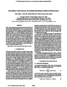
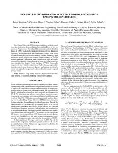
This paper presents a method of learning deep AND-OR Grammar (AOG) networks for visual recognition, which we term AOGNets. An AOGNet consists of a number of stages each of which is composed of a number of AOG building blocks. An AOG building block is designed based on a principled AND-OR grammar and represented by a hierarchical and compositional AND-OR graph [33, 46]. Each node applies some basic operation (e.g., Conv-BatchNormReLU) to its input. There are three types of nodes: an AND-node explores composition, whose input is computed by concatenating features of its child nodes; an OR-node represents alternative ways of composition in the spirit of exploitation, whose input is the element-wise sum of features of its child nodes; and a Terminal-node takes as input a channel-wise slice of the input feature map of the AOG building block. AOGNets aim to harness the best of two worlds (grammar models and deep neural networks) in representation learning with end-to-end training. In experiments, AOGNets are tested on three highly competitive image classification benchmarks: CIFAR-10, CIFAR-100 and ImageNet-1K. AOGNets obtain better performance than the widely used Residual Net [14] and most of its variants, and are comparable to the Dense Net [18]. AOGNets are also tested in object detection on the PASCAL VOC 2007 and 2012 [8] using the vanilla Faster RCNN [30] system and obtain better performance than the Residual Net.
AOG building block
And-node Or-node Terminal-node
Image
Channels
Figure 1. Illustration of the proposed AOGNet using the first AOG building block. The input feature map is treated as a sentence of N words (e.g., N = 4). The AND-OR graph of the building block is constructed to explore all possible parses of the sentence w.r.t. a simple binary composition rule. Each node applies some basic operation (e.g., Conv-BatchNorm-ReLU) to its input. There are three types of nodes: an AND-node explores composition, whose input is computed by concatenating features of its child nodes; an OR-node represents alternative ways of composition in the spirit of exploitation, whose input is the element-wise sum of features of its child nodes; and a Terminal-node takes as input a channel-wise slice of the input feature map (i.e., a k-gram). Note that the output feature map usually has smaller spatial dimensionality through the sub-sampling used in the Terminal-node operations and larger number of channels. The building block can be stacked to form deep hierarchy. See text for details. (Best viewed in color)
1. Introduction 1.1. Motivation and Objective Recently, deep neural networks [26, 22] improved prediction accuracy significantly in many vision tasks, and even obtained superhuman performance in image classification tasks [14, 36, 18, 6]. Much of these progress have been achieved mainly through engineering network architectures which can enjoy increasing representational power (by going either deeper or wider) without sacrificing the feasi∗ T.
Input feature map
bility of optimization using back-propagation with stochastic gradient descent (i.e., handling the vanishing and/or exploding gradient problem). On the one hand, although network engineering has been an active part of neural network research since their initial development, the overall architecture are still similar to the seminal work of Fukushi-
Wu is the corresponding author.
1
Softmax
Pooling
Convolution
“Laptop”
Figure 2. Illustration of an AOGNet which has 3 stages, 1 AOG building bock in the first and third stage, and 2 AOG building blocks in the second stage. Note that different stages can use different AND-OR graphs. We show the same one for simplicity. We also note that before entering the first AOG stage we can apply multiple steps of Conv-BatchNorm-ReLu or front-end stages from other networks such as residual nets. Thus, the proposed AOGNets can be integrated with many other networks. (Best viewed in color)
mas neocognitron [10]. Whether architecture are handcrafted [22, 4, 36, 14, 18, 6] or learned through architecture search [47], the process of finding the right architecture for a task requires significant effort for each individual case. On the other hand, the dramatic success does not necessarily speak to its sufficiency, let alone optimality, given the lack of theoretical underpinnings of deep neural networks at present [1]. Different methodologies are worth exploring to enlarge the scope of network architectures, and to potentially address the long-standing interpretability problem. For example, Hinton recently pointed out a crucial drawback of current convolutional neural networks: according to recent neuroscientific research, these artificial networks do not contain enough levels of structure [16, 32]. The wisdom in designing better deep network architectures usually lies in finding a network topology which can support both exploring new features and exploiting existing features in previous layers. From the perspective of representation learning, skip-connections within a Residual Network (ResNet) [14] contributes to effective features exploitation/reuse, and dense connection with feature maps being concatenated together in the densely connected network (DenseNet) [18] leads to effective feature exploration, beside their contributions in resolving the gradient vanishing and/or exploding issues in optimization. The Dual Path Network (DPN) [6] proposed a simple yet effective architecture which alternates skip connection and dense connection in forming network structure. This paper presents a method of integrating compositional grammar and deep neural networks in a deeply collaborative manner in representation learning, which naturally embraces the wisdom, thus harnesses the best of both worlds in representation learning and potentially opens the door of introducing more levels of structures based on well-studied, sophisticated, yet intuitive grammar models and structured knowledge representation [38] in deep representation learning. Grammar models are well known in both natural language processing and computer vision. Image grammar [46, 9, 45] was one of the dominant methods in computer vision before the recent resurgence in popularity of deep neural networks. With the recent resurgence, one fundamen-
tal puzzle arises that grammar models with more explicitly compositional structures and more analytic and theoretical potential, often perform worse than their neural network counterparts. The proposed method bridges the performance gap, which is motivated by and aims to show the advantage of two nice properties of grammar which are desirable in network engineering: (i) The flexibility and simplicity of constructing different types of structure topology based on a dictionary of primitives and a set of production rules in a principled way; and (ii) The highly expressive power and the parsimonious compactness of its explicitly hierarchical and compositional structure. Furthermore, the explainable rigor of grammar could be harnessed potentially to address the intepretability issue of deep neural networks (which is out of the scope of this paper).
1.2. Method Overview In this paper, we utilize compositional AND-OR grammar (AOG) in network engineering. We follow the general AND-OR grammar framework [46, 45] and specifically adopt the method presented in [33, 39] in constructing the grammar. We term the proposed deep compositional AOG networks AOGNets. An AOGNet consists of a stack of AOG building blocks. An AOG building block is designed based on a simple AND-OR grammar and represented by a hierarchical and compositional AND-OR graph [33, 39] (see Figure 1). Figure 2 illustrates a 3-stage AOGNet. The key idea of an AOG building block is to take advantage of both the exploration of new features and the exploitation/reuse of previously computed features in a hierarchical and compositional way, going beyond the pure skipconnection, the pure dense connection and their sequential combination. The proposed method is actually very simple. Given an input feature map with the number of channels being C, we first chunk it evenly into a small number N of primitive maps (e.g., N = 4 in Figure 1), then treat the input feature map as a sentence of N words. The AOG is constructed to explore all possible parse graphs of the sentence using only binary composition rules. Starting from the entire sentence, it is represented by an OR-node which can be either grounded on the entire input feature map or de-
composed in two child nodes (i.e., two sub-sentences) with respect to different splits. The former is represented by a Terminal-node and each of the latter is represented by an AND-node with two child nodes. The same is done recursively for the decomposed sub-sentences until no splits are available. Then, all the nodes are organized into a directed acyclic AND-OR graph. This is a 1-D special case of the method presented in [33, 39]. It can also be understood as a modified version of the well-known Cocke-YoungerKasami (CYK) parsing algorithm in natural language processing according to a binary composition rule. In the AOG, a Terminal-node takes as input a k-gram phrase consisting of k words (i.e., a slice of the feature map with the number of channels being k) where 1 ≤ k ≤ N . Then, we compute inputs of AND-nodes using the concatenation scheme as done in DenseNets [18] and OR-nodes using the summation scheme as done in ResNets [14]. Different variants of implementation of the two schema can be used in practice. Conceptually, an AOG building block embodies an exploration-and-exploitation-driven compositional structure for representation learning by deep neural networks. The AOG structure inherently embraces the skipconnection for words (chunks of feature maps) and the sentence itself (the entire input feature map) in a compositional way. We notice that we can extend the binary composition rule to explore larger space of network structures in a straightforward way subject to the GPU memory available in experiments (which is out of the scope of this paper). In experiments, we test our AOGNets on three highly competitive and widely used image classification benchmarks: the CIFAR-10 dataset and the CIFAR100 dataset [21], and the ImageNet-1000 dataset [31]. Our AOGNets obtain better performance consistently than ReslNets [14] and some variants, and are tightly comparable to DenseNets [18]. We further test AOGNets in object detection on the PASCAL VOC 2007 and 2012 [8]. We adopt the vanilla Faster RCNN [30] system using AOGNets as backbone. We obtain better performance than the one with ResNet as the backbone. We also provide a detailed ablation study analyzing different aspects of our AOGNets.
2. Related Work Network engineering is one of the most important and challenging hyper-parameter optimization problems in deep learning due to its significant contributions in improving performance. Network architecture search can be posed as a combinatorial search problem in a product space which consists of two sub-spaces: the structure space exploring all directed acyclic graphs with the start node representing input image and the end node representing task loss functions(s), and the operator space exploring all possible functions for implementing nodes in a searched structure. It is a extremely difficult problem due to the exponentially large
space and overall highly non-convex non-linear objective functions to be optimized in the search. We focus on convolutional networks in computer vision tasks in reviewing related work. The majority of existing methods are still based on hand-crafted architectures. A promising trend is to automatically learn better architectures with the long-term objective to have theoretical guarantee. So far, hand-crafted ones have better overall performance, especially on largescale datasets such as the ImageNet benchmark [31]. Hand-crafted network architectures. After more than 20 years since the seminal work 5-layer LeNet5 [26] was proposed, the recent resurgence in popularity of neural networks was triggered by the 8-layer AlexNet [22] with breakthrough performance on ImageNet [31] in 2012. The AlexNet presented two new insights in the operator space: the Rectified Linear Unit (ReLu) and the Dropout. Since then, a lot of efforts were devoted to learn deeper AlexNetlike networks with the intuition that deeper is better. The VGG Net [4] proposed a 19-layer network with insights on using multiple successive layers of small filters (e.g., 3 × 3) to obtain the receptive field by one layer with large filter and on adopting smaller stride in convolution to preserve information. A special case, 1 × 1 convolution, was proposed in the network-in-network [27] for reducing or expanding feature dimensionality between consecutive layers, and have been widely used in many networks. The VGG Net also increased computational cost and memory footprint significantly. To address these issues, The 22layer GoogLeNet [37] introduced the first inception module and a bottleneck scheme implemented with 1 × 1 convolution for reducing computational cost. The main obstacle of going deeper lies in the gradient vanishing issue in optimization, which is addressed with a new structural design, short-path or skip-connection, proposed in the Highway network [34] and popularized by the residual networks [14], especially when combined with the batch normalization [20]. More than 100 layers are popular design in the recent literature [14, 36], and even more than 1000 layers trained on large scale datasets such as ImageNet are not rare any more [19, 44]. The Fractal Net [25] provided an alternative way of implementing short path for training ultra-deep networks without residuals. Complementary to going deeper, width matters in residual networks and inception based networks too [43, 41]. Going beyond simple skip-connections, The densely connected network [18] proposed a densely connected network architecture with concatenation scheme for feature reuse and exploration, and the Dual Path Network [6] proposed to combine residuals and densely connections in an alternating way for more effective feature exploration and exploitation. Both skipconnection and dense-connection adapt the sequential architecture to directed and acyclic graph (DAG) structured networks, which were explored earlier in the context of re-
current neural networks (RNN) [2, 13] and ConvNets [42]. Most work focused on boosting spatial encoding and utilizing spatial dimensionality reduction. The squeeze-andexcitation module [17] is recently proposed a simple yet effective method focusing on channel-wise encoding. The Hourglass network [29] proposed a hourglass module consisting of both subsampling and upsampling to enjoy repeated bottom-up/top-down feature exploration. The proposed AOGNet belongs to hand-crafted architectures in general, but it is guided by intuitively simple yet principled grammar models. It shares some spirit with the inception module, the fractal net and the squeeze-andexcitation module. Thanks to its hierarchical and compositional structure, AOGNet is capable of balancing depth and width subject to a few hyper-parameters in constructing the AOG building blocks. It also enjoys both exploring new features and exploiting existing features in a compositional way, as well as taking advantage of channel-wise encoding. Learned network architectures. There is less work on this direction. Even with very strong assumptions (e.g., limited number of stages and limited set of operators), the search space still grows exponentially due to the product space. Bayesian hyper-parameter optimization is one of the popular methods for network architecture search in some restricted space [3, 28]. More recently, by posing the structure and connectivity of a neural network as a variable-length string, the network architecture search work [47] utilizes a recurrent network to generate a such string (i.e., network topology) under the reinforcement learning framework with the validation accuracy of intermediate models as reward. This automatic exploration of network topology entails very high demand on computing resource (e.g., 800 GPUs used in the experiments). Genetic algorithms are also explored in learning network structures [40]. In [7], the AdaNet was proposed to learn directed acyclic network structures using a theoretical framework with some guarantee. The proposed AOG building block is potentially useful as a better heuristic in the search or to facilitate theoretical analyses by taking advantage of the simple production rule in structure composition. Grammar-like structures. A general framework of image grammar was proposed in [46]. Object detection grammar was the dominant approaches for object detection [9, 33]. Probabilistic program induction [35, 23, 24] has been used successfully in many settings, but has not shown good performance in difficult visual understanding tasks such as large-scale image classification and object detection. More recently, recursive cortical networks [11] have been proposed with much more data efficiency in learning which adopts the AND-OR grammar framework [46], showing great potential of grammar like structures in developing general AI systems. Our contributions. This paper makes two main contri-
butions in the field of deep representation learning: • It presents a simple yet effective method of deeply integrating grammar models and deep neural networks, which facilitates both feature exploration and exploitation in a hierarchical and compositional way with nice balance between depth and width. In implementation, we adopt the AND-OR grammar (AOG) [33, 46, 45]. To the best of our knowledge, it is the first work that utilizes grammar models in network engineering. It sheds light on introducing more sophisticated structured knowledge representation [38] in network architecture search. • It shows better performance than state-of-the-art ResNets in both image classification and object detection. Paper Organization. The remainder of the paper is organized as follows. Section 3 presents details of our AOGNets. Section 4 shows experimental results and comparisons, as well as ablation studies on different aspects of our AOGNets. Finally, Section 5 concludes this paper and discusses some potential improvement.
3. AOGNets In this section, we first present details of constructing the structure of our AOGNets. Then, we define the operators for nodes in an AOGNet.
3.1. The Structure of an AOGNet An AOGNet consists of M stages (M ≥ 1). A stage l is composed of a small number nl of AOG building blocks (l ∈ [0, M − 1] and nl ≥ 1). Both M and nl ’s are predefined for a given task in learning. Figure 2 shows an AOGNet with M = 3, n1 = n3 = 1, n2 = 2. As illustrated in Figure 1, an AOG building block maps an input feature map F with the dimensionality C × H × W (representing the number of channels, height and width respectively) to an output feature map F with the dimensionality C × H × W. We treat the input feature map as a sentence of N words (or a filter bank with N primitives). Each word represents a primitive feature map with the dimensionality c × H × W in the input, satisfying C = N × c. In implementation, following a common convention, we usually reduce the spatial size and increase the number of channels between consecutive stages for bigger receptive field and greater expressive power. Within a stage, we usually keep the dimensionalities of input and output same for the AOG building blocks except for the first one. Constructing the AND-OR graph in an AOG building block. We consider the following three rules in unfolding
• The second rule is a binary decomposition (or composition) rule which decomposes the non-terminal sym-
• For an AND-node Ai,j (m), its input is computed by the concatenation of the outputs of its two child L R A nodes, fi,i+m and fi+m+1,j . We have fi,j = L R [fi,i+m , fi+m+1,j ]. • For an OR-node Oi,j , its input is thePsummation of the O u outputs of its child nodes, fi,j = ui,j ∈ch(Oi,j ) fi,j , where ch(·) be the set of child nodes.
(𝑐′, 1,1, 𝑠)
And-node / Or-node
O
ReLu
Bat
Linear
• The first rule is a termination rule which grounds the non-terminal symbol Si,j directly to the corresponding sub-sentence ti,j , i.e., a k-gram terminal symbol, which is represented by a Terminal-node in the ANDOR graph.
Pooling
Convolution
𝒯(𝐹/,0 ) 𝒯(𝒇 Initialization: Create an OR-node O0,N −1 for the Grounding Concatenation Summation entire sentence, V = {O0,N −1 }, E = ∅, BFS queue Q = {O0,N −1 }; … 𝑓/,0 = 𝐹/,0 𝒇8/,/67 𝒇}; and Right: an OR-node sums up the outputs of its child nodes. The same type of operator T () is applied to compute the outputs. ii) Create AND-nodes Ai,j (m) for all valid Output feature map splits 0 ≤ m < k; E = E ∪ {< vi,j , Ai,j (m) >}; bol Si,j into two child symbols representing a left subAOG building block if Ai,j (m) ∈ / V then sentence and a right sub-sentence respectively: Li,i+m V = V ∪ {Ai,j (m)}; and Ri+m+1,j , both of which are either a non-terminal Push Ai,j (m) to the back of Q; symbol or a terminal symbol depending on m. It is repAnd-node end Or-node resented by an AND-node in the AND-OR graph and Terminal-node else if vi,j is an AND-node with split index m then entails the concatenation scheme in forward compuCreate two OR-nodes Oi,i+m and Oi+m+1,j tation. for the two sub-sentence respectively; • The third rule represents alternative ways of decomE = E ∪ {< vi,j (m), Oi,i+m >, < posing a symbol Si,j , which is represented by an ORvi,j (m), Oi+m+1,j >}; feature map node in theInput AND-OR graph and entails summation Image if Oi,i+m ∈ / V then scheme in forward computation to “integrate out” the V = V ∪ {Oi,i+m }; Channels decomposition structures. Push Oi,i+m to the back of Q; end The AND-OR graph is constructed by a simple Algorithm 1 if Oi+m+1,j ∈ / V then using the breadth-first search (BFS). For example, we have V = V ∪ {Oi+m+1,j }; 10 Terminal-nodes, 10 AND-nodes and 6 OR-nodes for a Push Oi+m+1,j to the back of Q; small AOG with N = 4 as shown in Figure 1. end 3.2. The Operators in an AOGNet end end In an AOG building bock, each node in the AND-OR graph is implemented with some basic operator in a unified Algorithm 1: Constructing the AND-OR graph way. For a node vi,j in the AND-OR graph with length v v k = j − i + 1, denote by fi,j its input feature map, and fi,j the configurations of a sentence with N words: its output feature map. Denote by T () the operator mapping v v v fi,j to fi,j = T (fi,j ) (e.g., which can be implemented by Si,j → ti,j , (1) Conv-BatchNorm-ReLU). As shown in Figure 3, we have, Si,j (m) → Li,i+m · Ri+m+1,j , 0 ≤ m < k, (2) • For a Terminal-node ti,j , denote by Fi,j the correSi,j → Si,j (0)|Si,j (1)| · · · |Si,j (j − i). (3) sponding k-gram chunk in the input feature map F . t We have its input fi,j = Fi,j with the dimensionality where Si,j represents a symbol for unfolding the subv t c × H × W , and its output fi,j = T (Fi,j ) with the i,j sentence starting at the i-th word (i ∈ [0, N −1]) and ending v dimensionality c × H × W, where cvi,j = k × c and i,j at the j-th word (j ∈ [0, N − 1], j ≥ i) and its length equals C v ci,j = k × N . k = j − i + 1.
“Lap
(𝑐′, 1,1, 𝑠)
Output: 𝑐′×𝐻′×𝑊′
⊕
BatchNorm
(𝑐′, 1,1,1)
(𝑐′×𝛼, 3,3, 𝑠)
(𝑐′×𝛼, 1,1,1)
Input: 𝑐×𝐻×𝑊
Convolution
or Identity if 𝑐 = 𝑐′
ReLU
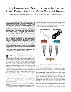
Figure 4. Illustration of the bottleneck operator. The 4-tuple of convolution represents (number of channels, kernel height, kernel width, stride). α is the bottleneck ratio (e.g., α = 0.25). The stride s is determined by the spatial sizes of input and output feature maps. (Best viewed in color)
Where the input and output of an AND-node or an ORnode, vi,j , have the same dimensionalities: cvi,j × H × W C and cvi,j = k × N . In learning and inference, we follow the depth-first search (DFS) order to compute nodes in an AOG building block, which ensures that all the child nodes have been computed when we compute a node v. We notice that we can apply different operators for different types of nodes as long as we can match the dimensionalities during the computation. We keep it simple in this paper. In our experiments, we use both standard ConvBatchNorm-ReLU and a so-called bottleneck operator as done in the Residual Nets [14]. We leave the exploration of different operators in future work. Short Path in an AOGNet. The hierarchical and compositional structure of an AND-OR graph facilitates very diverse information flows in learning. In an AOG building bock, every primitive feature map (i.e., one word) goes through multiple paths to the output feature map: some are short and some are long. For example, every primitive feature map is directly connected with the root OR-node. Balance between Depth and Width. The hierarchical and compositional structure of an AND-OR graph also leads to good balance between depth and width in the network architecture.
4. Experiments In this section, we test our AOGNets on three highly competitive image classification benchmarks: CIFAR-10 and CIFAR-100 [21], and ImageNet-1K [31], and on the PASCAL VOC 2007 and 2012 benchmarks [8]. We first present an ablation study of two important hyperparameters of AOGNets on CIFAR-100. Then, we show detailed experimental results and analyses of our AOGNets on
Figure 5. Left: Comparison of the parameter efficiency between Conv-BatchNorm-ReLU and bottleneck (BN) operators. Right: Comparison between primitive size N from 2 to 6 with different parameter sizes. Both are measured using the CIFAR-100 test error. (Best viewed in color)
image classification and object detection tasks. We implemented our AOGNets using the latest version of MXNet [5]. Our source code will be released soon. AOGNet Settings. We use two different node operator T ()’s in our experiments. One is the standard ConvBatchNorm-ReLU, and the other one is the so-called bottleneck (BN) operator (see Figure 4) used in the ResidualNet [14] and its variants. In comparison, AOGNets will be written by AOGNet-[BN]-PrimitiveSize-(#AOG blocks per stage). For example, AOGNet-4-(1,1,1) and AOGNet-BN4-(1,1,1) represent a 3-stage AOGNet using standard node operator and bottleneck one respectively, both with primitive size being 4, and 1 AOG building block per stage. After the structure is specified, the number of parameters of an AOGNet is determined by the number of channels of input/output of each stage. Thus, for an M -stage AOGNet, we have an (M + 1)-tuple specifying the number of channels. For example, we can specify the 4-tuple, (16, 16, 32, 64) or (16, 32, 64, 128) for a 3-stage AOGNet4-(1,1,1), resulting different number of parameters in total. The depth of an AOGNet is defined by the largest number of units which have learnable parameters along the paths from the final output to the input data following BFS order (e.g., a BN operator as shown in Figure 4 is counted as 3 units).
4.1. Ablation Study on CIFAR-100 The structural complexity of an AOGNet depends on both the total number of AOG building blocks and the primitive sizes of AOG building blocks (which fully control the AND-OR graph, see Algorithm 1). After the structure is specified, the model complexity and expressive power largely depend on node operators. We conduct an ablation study of these two aspects on CIFAR-100 as follows. Bottleneck Node Operator for Parameter Efficiency. The left plot in Figure 5 compares the parameter efficiency between the two node operators used in this paper: ConvBatchNorm-ReLU and bottleneck (BN). In comparisons,
we use 3-stage AOGNets with a single type of AOG building block whose primitive size is 4. Specially, we compare AOGNet-4-(1,1,1) and AOGNeet-BN-4-(1,1,1) with the total number of parameters being 1M, 2M, 4M, and 8M respectively (M represents the unit of Million), and compare AOGNet-4-(1,2,1) and AOGNet-BN-4-(1,2,1) with 16M parameters. BN operator consistently outperforms the counterpart by more than 2% with the same model structure and complexity, thus it is more efficient in terms of the number of parameters. It is worth noting that the ConvBatchNorm-ReLU results uses a dropout layer with dropout rate 0.1 after each Conv-BatchNorm-ReLU operation similar to DenseNet [18]. And the dropout layers result in about 0.8% improvement on the test accuracy, while BN does not need the dropout regularization to improve accuracy. In other words, our AOGNet-BN is less prone to overfitting. Primitive Size vs. Channel Width. We further compare AOGNets-BN with different primitive sizes across different model complexities. The right plot in Figure 5 shows comparisons of AOGNet-BN-N -(1, 1,1) between 5 different primitive size, N = 2, · · · , 6 with 5 different model complexities (1M, 2M, 4M, 8M and 16M ). To control the model complexity of AOGNets-BN with different primitive sizes, we adjust the number of channels of input/output feature maps accordingly. Overall, we empirically observe that N = 4 gives the best performance. We note that when the number of parameter is sufficiently large we think that bigger the primitive size is better the performance is with proper hyper-parameter tuning (such as learning rate and batch size). Based on the ablation study, we fix the primitive size to N = 4 in all experiments and use BN operator only on ImageNet for the sake of saving GPU hours.
4.2. Experiments on CIFAR CIFAR-10 and CIFAR-100 datasets [21], denoted by C10 and C100 respectively, consist of 32 × 32 color images drawn from 10 and 100 classes. The training and test sets contains 50,000 and 10,000 images respectively. We adopt widely used standard data augmentation scheme, random cropping and mirroring, in preparing the training data. We train AOGNets with stochastic gradient descent (SGD) for 300 epochs with parameters initialized by the Xavier method [12]. The initial learning rate is set to 0.1, and is divided by 10 at 150 and 225 epoch respectively. For CIFAR-10, we chose batch size 64 with weight decay 1 × 10⁻⁴ , while batch size 128 with weight decay 5 × 10⁻⁴ is adopted for CIFAR-100. The momentum is set to 0.9. If the network uses only Conv-BatchNorm-ReLU (without bottleneck), a dropout layer of dropout ratio 0.1 is applied after each Conv-BatchNorm-ReLU block. Results and Analyses. We summarize the results in Table 1. Our AOGNets obtain better performance than
Method ResNet [14] ResNet (reported by [19]) ResNet (pre-activation) [15] Wide ResNet [43] FractalNet [25] with Dropout/DropPath ResNeXt-29, 8 × 64d [41] ResNeXt-29, 16 × 64d [41] DenseNet [18] (k = 12) DenseNet [18] (k = 12) DenseNet [18] (k = 24) DenseNet-BC [18] (k = 12) DenseNet-BC [18] (k = 24) DenseNet-BC [18] (k = 40) AOGNet-4-(1,1,1) AOGNet-4-(1,1,1) AOGNet-4-(1,1,1) AOGNet-4-(1,2,1) AOGNet-BN-4-(1,1,1) AOGNet-BN-4-(1,1,1) AOGNet-BN-4-(1,2,1) AOGNet-BN-4-(1,2,1)
Depth 110 110 164 1001 16 28 21 21 29 29 40 100 100 100 250 190 23 23 23 37 65 65 86 86
#Params 1.7M 1.7M 1.7M 10.2M 11.0M 36.5M 38.6M 38.6M 34.4M 68.1M 1.0M 7.0M 27.2M 0.8M 15.3M 25.6M 1.0M 8.1M 16.0M 32.1M 1.0M 8.0M 16.0M 32.5M
C10 6.61 6.41 5.46 4.62 4.81 4.17 5.22 4.60 3.65 3.58 5.24 4.10 3.74 4.51 3.62 3.46 5.29 4.02 3.79 3.74 4.74 3.99 3.78 3.66
C100 27.22 24.33 22.71 22.07 20.50 23.30 23.73 17.77 17.31 24.42 20.20 19.25 22.27 17.60 17.18 25.98 20.64 19.50 18.89 22.81 18.71 17.82 17.74
Table 1. Error rates (%) on the two CIFAR datasets [21]. #Params uses the unit of Million. k in DenseNet refers to the growth rate.
Method ResNet-101 [14] ResNet-152 [14] ResNet-200 [15] WRN-50-2-bottleneck [43] ResNeXt-101 [41] DensetNet-161 [18] (k = 48) DualPathNet-68 [6] DualPathNet-92 [6] AOGNet-BN-4-(1,1,1,1)
#Params 44.5M 60.2M 64.7M 68.9M 83.9M 27.9M 12.8M 38.0M 79.5M
top-1 23.6 23.0 21.7 21.9 20.4 22.2 23.57 20.73 21.49
top-5 7.1 6.7 5.8 6.03 5.3 6.93 5.37 5.76
Table 2. The top-1 and top-5 error rates (%) on the ImageNet-1K validation set using single model and single-crop testing.
Residual Nets [14] consistently on both datasets, and achieve comparable performance with the state-of-the-art DenseNets [18] and ResNeXt [41]. Our AOGNets outperform Residual Nets even without using BN operators, which shows the advantage of the hierarchical and compositional structure of AOG building blocks in representation learning. AOGNets are slightly worse than DenseNets and we think that the main reason is that AND-nodes in our current AOGNets consist of two child nodes only, thus are less expressive in terms of exploring new features by concatenating previous layers. One potential improvement of AOGNets could be obtained by concatenating the entire sub-graph rooted at each AND-node in learning, as well as by extending the binary composition rule in constructing AND-OR graphs. Another more straightforward way is to
07trainval/07test 07+12trainval/07test 07+12trainval/12test
Method ResNet-101∗ AOGNet-BN-4-(1,1,1,1) ResNet-101 [14] ResNet-101∗ AOGNet-BN-4-(1,1,1,1) ResNet-101∗ AOGNet-BN-4-(1,1,1,1)
mAP 74.7 77.6 76.4 78.4 81.2 75.1 77.9
areo 75.8 78.8 79.8 79.0 79.1 87.2 88.6
bike 81.6 83.4 80.7 81.9 86.5 83.1 85.7
bird 75.0 79.3 76.2 78.6 81.4 74.5 79.4
boat 67.4 66.1 68.3 69.1 73.4 60.1 66.6
bottle bus 60.1 81.4 65.2 85.9 55.9 85.1 66.4 85.5 70.5 87.4 58.3 80.3 63.2 83.6
car 85.6 87.4 85.3 87.9 88.9 80.1 82.2
cat 84.7 87.3 89.8 88.5 88.8 90.8 92.4
chair 59.7 62.6 56.7 65.0 68.4 57.5 59.0
cow 79.7 86.2 87.8 84.4 87.0 79.4 80.6
table 69.4 70.0 69.4 73.6 77.4 60.7 62.7
dog 84.4 87.6 88.3 85.6 88.3 88.7 90.4
horse 83.8 87.2 88.9 87.2 89.3 84.2 88.0
mbike person plant 79.3 79.1 47.6 81.6 79.5 51.7 80.9 78.4 41.7 84.3 79.7 50.9 85.1 83.5 55.6 84.1 82.6 52.5 85.7 84.7 57.6
sheep 73.7 77.7 78.6 77.6 83.8 76.9 79.7
sofa 74.1 78.0 79.8 80.1 82.2 67.4 70.0
train 77.9 80.7 85.3 85.3 86.1 84.4 87.2
tv 74.6 75.9 72.0 77.8 81.2 68.3 71.8
Table 3. Performance comparisons using Average Precision (AP) at the intersection over union (IoU) threshold 0.5 (
[email protected]) in the PASCAL VOC2007 / VOC2012 dataset (using the protocol, competition ”comp4” trained with ImageNet pretrained models and using only 2007 trainval or both 2007 and 2012 trainval datasets). ∗ reported based on our re-implementation for fair comparisons. The results evaluated by the VOC2012 test server can be viewed at http://host.robots.ox.ac.uk:8080/anonymous/XHO7OS.html (AOGNet-BN-4-(1,1,1,1)) and http://host.robots.ox.ac.uk:8080/anonymous/XMV4AI.html (ResNet-101).
adopt the inception module [36] like node operators as done by the ResNeXt [41] w.r.t. ResNet [14] at the expense of increasing model complexity significantly. We will investigate both of them in future work.
4.3. Experiments on ImageNet-1K The ILSVRC 2012 classification dataset [31] consists of about 1.2 million images for training, and 50,000 for validation, from 1,000 classes. We adopt the same data augmentation scheme for training images as done in [14, 15, 18], and apply a single-crop with size 224 × 224 at test time. Following the common protocol, we evaluate the top-1 and top-5 classification error rates on the validation set. We use AOGNet-BN with four stages for training the ImageNet-1K dataset. Before entering the first AOG stage, a 7 × 7 convolution layer with stride 2 and filter size 64 is performed on the input image, and followed by a 3 × 3 max pooling layer with stride 2. Similar to the network structure for training CIFAR, in the first AOG block of each stage s (s ≥ 2), the convolution operation of all the terminal nodes in that block is performed with a stride 2. The intermediate and output feature map sizes in the four stages are 56 × 56, 28 × 28, 14 × 14 and 7 × 7. The output channel width of each four stages is set as 256, 512, 1024 and 2048. We train the AOGNet with stochastic gradient descent (SGD) for 120 epochs with parameters initialized by the Xavier method [12]. The initial learning rate is set to 0.1, and is divided by 10 at 30, 60 and 90 epoch respectively. We set the batch size to 256 with weight decay 1 × 10⁻⁴ and momentum 0.9. Results and Analyses. Results and comparisons are shown in Table 2. Our AOGNets obtain better performance than Residual Nets with comparable model complexities, and are comparable to ResNeXt. We did not test the standard node operators on ImageNet-1K since bottleneck based node operators are consistently better on CIFAR datasets and we do not have enough GPU computing resource to train multiple models on ImageNet-1k before submission. Although we obtain slightly better performance than DenseNet and ResNet-200, our AOGNets use more number of parameters than ResNet-200, and much
more than DenseNet. Dual Path Nets [6] outperform our AOGNets in terms of both accuracy and model complexity. To reduce the model complexity, we will investigate methods similar to the growth rate used in DenseNets and Dual Path Nets when extending the binary composition rule and applying the sub-graph based concatenation schema for AND-nodes (as stated above). Furthermore, in our experiments, we used the same initial learning rate, the same initialization method for parameters of the three types of nodes, and other settings as done in training ResNet for fair comparisons. Tuning those hyper-parameters w.r.t. our AOGNets could improve performance potentially on ImageNet, which requires sufficiently large GPU computing resources of which we are short at present.
4.4. Object Detection on PASCAL VOC We test the proposed AOGNets in object detection on the PASCAL VOC 2007 and 2012 datasets [8]. We adopt the vanilla Faster RCNN system [30] and reuse the code in MXNet 1 . We only substitute the ConvNet backbone with our AOGNets in experiments and keep everything else unchanged for fair comparison. We use the 4-stage AOGNetBN-4-(1,1,1,1) pretrained on ImageNet. We adopt the endto-end training procedure implemented in MXNet to train the region proposal network (RPN) and RCNN jontly. The first three stages are shared by RPN and RCNN, and the last stage is used as the head classifier for region-of-interest (RoI) prediction. We fix all parameters pretrained on ImageNet before stage 1 (inclusive) in training. We follow standard evaluation metrics Average Precision (AP) and mean of AP (mAP) in the PASCAL challenge protocols for evaluation [8]. Table 3 shows the detection results and comparisons. Our AOGNets obtain better mAP than ResNet-101 by more than 2% consistently.
5. Conclusions and Discussions This paper presented deep AND-OR grammar (AOG) networks for visual recognition which, we term AOGNets, consist of a number of stages of AOG building blocks. The 1 MXNet implmentation of Faster RCNN:https://github.com/ apache/incubator-mxnet/tree/master/example/rcnn
AOG building block is a simple yet effective representation learning module implemented by a directed acyclic ANDOR graph adapted from [33, 39], which can explore new features and exploit previously computed features in a hierarchical and compositional way, thus shed light on addressing the long-standing network architecture search problem in deep learning. The proposed AOGNets are tested on three highly competitive image classification benchmarks, CIFAR-10 and CIFAR-100 [21], and ImageNet1k [31]. AOGNets obtain better performance than Residual Nets [14] and most of their variants, and are comparable with the latest ResNeXt [41] and DenseNets [18]. AOGNets are also tested on PASCAL VOC 2007 and 2012 [8] using the vanilla Faster RCNN [30] system, and obtain better performance than Residual Nets. Discussions. We hope this paper encourages further exploration in integrating compositional grammar models and other structured knowledge representation and deep neural networks end-to-end, especially to harness the explainable rigor of the former and the discriminative power of the latter. In implementation, some interesting aspects that worth investigating include, but not limited to, searching better hyper-parameters in learning AOGNets (e.g., learning rate and schedule, parameter initialization and batch size, etc), conducting experiments with much larger AOGNets (deeper and wider with different primitive size per stage), extending binary composition rule in constructing AND-OR graphs, adopting sub-graph based concatenation scheme for ANDnodes with predefined growth rate as done in DenseNet and DPN, and using front-end stages from networks such as ResNet, DenseNet and DPN before the first stage to further boost the experssive power and to save memory footprint.
[6]
[7]
[8]
[9]
[10]
[11]
[12]
[13]
References [1] S. Arora, A. Bhaskara, R. Ge, and T. Ma. Provable bounds for learning some deep representations. In Proceedings of the 31th International Conference on Machine Learning, ICML, pages 584–592, 2014. 2 [2] P. Baldi and G. Pollastri. The principled design of large-scale recursive neural network architectures–dag-rnns and the protein structure prediction problem. Journal of Machine Learning Research, 4:575–602, 2003. 3 [3] J. Bergstra, D. Yamins, and D. D. Cox. Making a science of model search: Hyperparameter optimization in hundreds of dimensions for vision architectures. In Proceedings of the 30th International Conference on Machine Learning, ICML 2013, Atlanta, GA, USA, 16-21 June 2013, pages 115–123, 2013. 4 [4] K. Chatfield, K. Simonyan, A. Vedaldi, and A. Zisserman. Return of the devil in the details: Delving deep into convolutional nets. In British Machine Vision Conference, BMVC, 2014. 2, 3 [5] T. Chen, M. Li, Y. Li, M. Lin, N. Wang, M. Wang, T. Xiao, B. Xu, C. Zhang, and Z. Zhang. Mxnet: A flexible and effi-
[14]
[15]
[16]
[17] [18]
cient machine learning library for heterogeneous distributed systems. CoRR, abs/1512.01274, 2015. 6 Y. Chen, J. Li, H. Xiao, X. Jin, S. Yan, and J. Feng. Dual path networks. arXiv preprint arXiv:1707.01629, 2017. 1, 2, 3, 7, 8 C. Cortes, X. Gonzalvo, V. Kuznetsov, M. Mohri, and S. Yang. Adanet: Adaptive structural learning of artificial neural networks. In Proceedings of the 34th International Conference on Machine Learning, ICML 2017, Sydney, NSW, Australia, 6-11 August 2017, pages 874–883, 2017. 4 M. Everingham, S. M. Eslami, L. Gool, C. K. Williams, J. Winn, and A. Zisserman. The pascal visual object classes challenge: A retrospective. Int. J. Comput. Vision (IJCV), 111(1):98–136, Jan. 2015. 1, 3, 6, 8, 9 P. F. Felzenszwalb. Object detection grammars. In IEEE International Conference on Computer Vision Workshops, ICCV, page 691, 2011. 2, 4 K. Fukushima. Neocognitron: A self-organizing neural network model for a mechanism of pattern recognition unaffected by shift in position. Biological cybernetics, 36(4):193–202, 1980. 2 D. George, W. Lehrach, K. Kansky, M. L´azaro-Gredilla, C. Laan, B. Marthi, X. Lou, Z. Meng, Y. Liu, H. Wang, A. Lavin, and D. S. Phoenix. A generative vision model that trains with high data efficiency and breaks text-based captchas. Science, 2017. 4 X. Glorot and Y. Bengio. Understanding the difficulty of training deep feedforward neural networks. In Proceedings of the Thirteenth International Conference on Artificial Intelligence and Statistics, AISTATS 2010, Chia Laguna Resort, Sardinia, Italy, May 13-15, 2010, pages 249–256, 2010. 7, 8 A. Graves and J. Schmidhuber. Offline handwriting recognition with multidimensional recurrent neural networks. In Advances in Neural Information Processing Systems 21, Proceedings of the Twenty-Second Annual Conference on Neural Information Processing Systems, Vancouver, British Columbia, Canada, December 8-11, 2008, pages 545–552, 2008. 3 K. He, X. Zhang, S. Ren, and J. Sun. Deep residual learning for image recognition. In IEEE Conference on Computer Vision and Pattern Recognition (CVPR), 2016. 1, 2, 3, 6, 7, 8, 9 K. He, X. Zhang, S. Ren, and J. Sun. Identity mappings in deep residual networks. In Computer Vision - ECCV 2016 - 14th European Conference, Amsterdam, The Netherlands, October 11-14, 2016, Proceedings, Part IV, pages 630–645, 2016. 7, 8 G. Hinton. What is wrong with convolutional neural nets? the 2017 - 2018 Machine Learning Advances and Applications Seminar presented by the Vector Institute at U of Toronto, https://www.youtube.com/watch?v=Mqt8fs6ZbHk, August 17, 2017. 2 J. Hu, L. Shen, and G. Sun. Squeeze-and-excitation networks. CoRR, abs/1709.01507, 2017. 4 G. Huang, Z. Liu, L. van der Maaten, and K. Q. Weinberger. Densely connected convolutional networks. In Proceedings of the IEEE Conference on Computer Vision and Pattern Recognition, 2017. 1, 2, 3, 7, 8, 9
[19] G. Huang, Y. Sun, Z. Liu, D. Sedra, and K. Q. Weinberger. Deep networks with stochastic depth. In Computer Vision ECCV 2016 - 14th European Conference, Amsterdam, The Netherlands, October 11-14, 2016, Proceedings, Part IV, pages 646–661, 2016. 3, 7 [20] S. Ioffe and C. Szegedy. Batch normalization: Accelerating deep network training by reducing internal covariate shift. In D. Blei and F. Bach, editors, Proceedings of the 32nd International Conference on Machine Learning (ICML-15), pages 448–456. JMLR Workshop and Conference Proceedings, 2015. 3 [21] A. Krizhevsky and G. Hinton. Learning multiple layers of features from tiny images. Master’s thesis, Department of Computer Science, University of Toronto, 2009. 3, 6, 7, 9 [22] A. Krizhevsky, I. Sutskever, and G. E. Hinton. Imagenet classification with deep convolutional neural networks. In Neural Information Processing Systems (NIPS), pages 1106– 1114, 2012. 1, 2, 3 [23] B. M. Lake, R. Salakhutdinov, and J. B. Tenenbaum. Humanlevel concept learning through probabilistic program induction. Science, 2015. 4 [24] B. M. Lake, T. D. Ullman, J. B. Tenenbaum, and S. J. Gershman. Building machines that learn and think like people. CoRR, abs/1604.00289, 2016. 4 [25] G. Larsson, M. Maire, and G. Shakhnarovich. Fractalnet: Ultra-deep neural networks without residuals. CoRR, abs/1605.07648, 2016. 3, 7 [26] Y. LeCun, L. Bottou, Y. Bengio, and P. Haffner. Gradientbased learning applied to document recognition. Proceedings of the IEEE, 86(11):2278–2324, 1998. 1, 3 [27] M. Lin, Q. Chen, and S. Yan. Network in network. CoRR, abs/1312.4400, 2013. 3 [28] H. Mendoza, A. Klein, M. Feurer, J. T. Springenberg, and F. Hutter. Towards automatically-tuned neural networks. In Proceedings of the 2016 Workshop on Automatic Machine Learning, AutoML 2016, co-located with 33rd International Conference on Machine Learning (ICML 2016), New York City, NY, USA, June 24, 2016, pages 58–65, 2016. 4 [29] A. Newell, K. Yang, and J. Deng. Stacked hourglass networks for human pose estimation. CoRR, abs/1603.06937, 2016. 4 [30] S. Ren, K. He, R. Girshick, and J. Sun. Faster R-CNN: Towards real-time object detection with region proposal networks. In Neural Information Processing Systems (NIPS), 2015. 1, 3, 8, 9 [31] O. Russakovsky, J. Deng, H. Su, J. Krause, S. Satheesh, S. Ma, Z. Huang, A. Karpathy, A. Khosla, M. Bernstein, A. C. Berg, and L. Fei-Fei. ImageNet Large Scale Visual Recognition Challenge. Int. J. Comput. Vision (IJCV), 115(3):211–252, 2015. 3, 6, 8, 9 [32] S. Sabour, N. Frosst, and G. E Hinton. Dynamic Routing Between Capsules. ArXiv e-prints, Oct. 2017. 2 [33] X. Song, T. Wu, Y. Jia, and S. Zhu. Discriminatively trained and-or tree models for object detection. In Proceedings of 2013 IEEE Conference on Computer Vision and Pattern Recognition (CVPR), pages 3278–3285, 2013. 1, 2, 3, 4, 9 [34] R. K. Srivastava, K. Greff, and J. Schmidhuber. Highway networks. CoRR, abs/1505.00387, 2015. 3
[35] P. D. Summers. A methodology for LISP program construction from examples. J. ACM, 24(1):161–175, 1977. 4 [36] C. Szegedy, S. Ioffe, and V. Vanhoucke. Inception-v4, inception-resnet and the impact of residual connections on learning. CoRR, abs/1602.07261, 2016. 1, 2, 3, 8 [37] C. Szegedy, W. Liu, Y. Jia, P. Sermanet, S. E. Reed, D. Anguelov, D. Erhan, V. Vanhoucke, and A. Rabinovich. Going deeper with convolutions. In IEEE Conference on Computer Vision and Pattern Recognition, CVPR 2015, Boston, MA, USA, June 7-12, 2015, pages 1–9, 2015. 3 [38] F. van Harmelen, V. Lifschitz, and B. W. Porter, editors. Handbook of Knowledge Representation, volume 3 of Foundations of Artificial Intelligence. Elsevier, 2008. 2, 4 [39] T. Wu, Y. Lu, and S. Zhu. Online object tracking, learning and parsing with and-or graphs. IEEE Trans. Pattern Anal. Mach. Intell. (PAMI), DOI: 10.1109/TPAMI.2016.2644963, 2016. 2, 3, 9 [40] L. Xie and A. L. Yuille. Genetic CNN. CoRR, abs/1703.01513, 2017. 4 [41] S. Xie, R. B. Girshick, P. Doll´ar, Z. Tu, and K. He. Aggregated residual transformations for deep neural networks. CoRR, abs/1611.05431, 2016. 3, 7, 8, 9 [42] S. Yang and D. Ramanan. Multi-scale recognition with dagcnns. In 2015 IEEE International Conference on Computer Vision, ICCV 2015, Santiago, Chile, December 7-13, 2015, pages 1215–1223, 2015. 4 [43] S. Zagoruyko and N. Komodakis. Wide residual networks. In Proceedings of the British Machine Vision Conference 2016, BMVC 2016, York, UK, September 19-22, 2016, 2016. 3, 7 [44] X. Zhang, Z. Li, C. C. Loy, and D. Lin. Polynet: A pursuit of structural diversity in very deep networks. CoRR, abs/1611.05725, 2016. 3 [45] L. Zhu, Y. Chen, Y. Lu, C. Lin, and A. L. Yuille. Max margin AND/OR graph learning for parsing the human body. In 2008 IEEE Computer Society Conference on Computer Vision and Pattern Recognition (CVPR), 2008. 2, 4 [46] S. C. Zhu and D. Mumford. A stochastic grammar of images. Foundations and Trends in Computer Graphics and Vision, 2(4):259–362, 2006. 1, 2, 4 [47] B. Zoph and Q. V. Le. Neural architecture search with reinforcement learning. In Proceedings of International Conference on Learning Representations, 2016. 2, 4