Apodizing functions for Fourier transform spectroscopy - University of ...

3644

J. Opt. Soc. Am. A / Vol. 24, No. 11 / November 2007

D. A. Naylor and M. K. Tahic

Apodizing functions for Fourier transform spectroscopy David A. Naylor* and Margaret K. Tahic Department of Physics, University of Lethbridge, 4401 University Drive, Lethbridge, Alberta, T1K 3M4, Canada *Corresponding author: [email protected] Received July 6, 2007; revised August 17, 2007; accepted August 22, 2007; posted August 27, 2007 (Doc. ID 84862); published October 30, 2007 Apodizing functions are used in Fourier transform spectroscopy (FTS) to reduce the magnitude of the sidelobes in the instrumental line shape (ILS), which are a direct result of the finite maximum optical path difference in the measured interferogram. Three apodizing functions, which are considered optimal in the sense of producing the smallest loss in spectral resolution for a given reduction in the magnitude of the largest sidelobe, find frequent use in FTS [J. Opt. Soc. Am. 66, 259 (1976)]. We extend this series to include optimal apodizing functions corresponding to increases in the width of the ILS ranging from factors of 1.1 to 2.0 compared with its unapodized value, and we compare the results with other commonly used apodizing functions. © 2007 Optical Society of America OCIS codes: 300.6300, 300.3700.

1. INTRODUCTION It is common practice in Fourier transform spectroscopy to multiply the measured interferogram by an apodizing function in order to reduce the amount of ringing present in the resulting instrumental line shape (ILS) [1]. Many apodizing functions have been reported in the literature [2–5], and practitioners often make their choice without a clear understanding of the role of the function on the independence of the resulting spectral data points [3]. While purists would question the need for apodizing in the first place, the reduction in the amplitude of the secondary maxima/minima of the ILS, albeit at the cost of lower spectral resolution, is often desired. In this paper we expand on the work of Norton and Beer [3,4] to generate a family of apodizing functions that are close to optimum, in the sense that, to a large degree, they preserve the orthogonal properties of the sinc function, provide near optimum reduction in the amplitude of the secondary maxima/minima for a given decrease in spectral resolution, and are simple to compute.

2. BACKGROUND The interferogram, I共␦兲, of a polychromatic source, B共␴兲, as measured with an ideal interferometer can be written as [1] I共␦兲 =

冕

B共␴兲 =

冕

+⬁

I共␦兲cos共2␲␴␦兲d␦ .

共2兲

−⬁

In practice, interferograms can only be measured out to finite optical path differences determined by the length of the translation stage of the interferometer. In the case of symmetrical optical path difference limits of ±L, Eq. (2) becomes B共␴兲 =

冕

+L

I共␦兲cos共2␲␴␦兲d␦ ,

−L

which is equivalent to multiplying Eq. (2) by the boxcar function: ⌸共␦兲 = 1,

兩␦兩 艋 L

⌸共␦兲 = 0,

兩␦兩 ⬎ L.

In Fourier analysis, multiplication in the spatial domain is equivalent to convolution in the spectral domain [1]. The effect of measuring the interferogram out to finite path differences is thus equivalent to convolving the input spectrum with the Fourier transform of the boxcar function: I兵⌸共␦兲其 =

冕

+L

cos共2␲␴␦兲d␦

−L

+⬁

B共␴兲关1 + cos共2␲␴␦兲兴d␴ ,

共1兲

=

2L sin共2␲␴L兲

−⬁

where ␦ is the optical path difference (cm) between the two interfering beams and ␴ is the frequency expressed in wavenumbers 共cm−1兲. It is customary to neglect the constant (DC) term in Eq. (1), in which case the spectrum is recovered via the inverse cosine Fourier transform: 1084-7529/07/113644-5/$15.00

2␲␴L

= 2L sinc共2␲␴L兲, which is the well-known sinc function. The sinc function has a full width at half maximum (FWHM) of 0.603/ L and is characterized by a series of secondary lobes of slowly decreasing amplitude, the amplitude of the first © 2007 Optical Society of America

D. A. Naylor and M. K. Tahic

Vol. 24, No. 11 / November 2007 / J. Opt. Soc. Am. A

3645

minimum being −21.7% of the main lobe. The goal of apodizing is to decrease the amplitudes of the sidelobes associated with the sinc function at the cost of increasing the FWHM of the ILS (i.e., decreasing the spectral resolution). Apodizing is readily accomplished by multiplying the interferogram with an apodizing function, A共␦兲, whose Fourier transform, when multiplied by any existing apodization (e.g., due to divergence or vignetting of the beams within the interferometer), becomes the new ILS.

3. COMPARING APODIZING FUNCTIONS During his extensive study Filler [2] devised a graphical method for comparing different apodizing functions and their corresponding ILS. This method graphs the normalized height of the absolute largest secondary lobe of the ILS, relative to the height of the absolute largest secondary lobe of the sinc function, against the FWHM of the ILS, again relative to the FWHM of the sinc function. (The absolute largest secondary lobe of an ILS need not necessarily be the first one and could be either a maximum or a minimum.) Filler introduced two families of apodizing functions, D␣共␦兲 and E␣共␦兲 (where ␦ is the optical path difference out to a maximum value of L), which are defined as

D␣

E␣

冉冊 ␦

L

冉冊 冉 冊 ␦

L

= cos

␲␦

2L

冉 冊

+ ␣ cos

冉 冊

= 1 + 共1 + ␣兲cos

␲␦ L

3␲␦ 2L

0 艋 ␣ 艋 1,

,

冉 冊

+ ␣ cos

2␲␦ L

0 艋 ␣ 艋 1,

,

which he considered to give superior performance to other commonly used functions. Norton and Beer [3] extended this analysis and introduced the functions, P␣,p共␦兲, variants of the E␣共␦兲 family, where

P␣,p

冉冊 ␦

L

冉 冊

= 1 + p + 共1 + ␣兲cos − 1 艋 ␣ 艋 1;

␲␦ L

冉 冊

+ ␣ cos

2␲␦ L

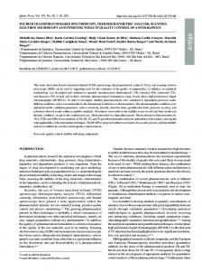
Fig. 1. (Color online) The profile of the extended apodizing functions.

冉冊

NB

␦

L

n

=

兺 i=0

冉 冉 冊冊

Ci 1 −

␦

2 i

L

,

n

where

兺 C = 1, i

共3兲

n = 0,1,2,3. . .

i=0

Norton and Beer used Eq. (3) to generate three functions corresponding to weak, medium, and strong apodization that produced near optimal reduction in the amplitude of the sidelobes for increases in the FWHM of the ILS corresponding to factors of 1.2, 1.4, and 1.6, respectively. The authors found no significant improvement in performance for n ⬎ 4, and in all cases C3 = 0. For completeness the coefficients of these three apodizing functions are presented in Table 1. The authors went on to show that the loci of these functions, when plotted on the Filler diagram, did not lie below the empirically boundary described by

冏冏 h

log

h0

冉 冊

⬇ 1.939 − 1.401

W

W0

冉 冊 W

− 0.597

W0

2

,

共4兲

where h / h0 is the absolute peak of the largest secondary maximum relative to that of the sinc function and W / W0 is the ratio of the FWHM of the resulting ILS, again relative to that of the sinc function. The authors issued a chal-

,

0 艋 p 艋 1.

While the functions P were judged to be superior to both D and E, by their loci on the Filler diagram, their convergence was rather slow. This provided the impetus for Norton and Beer to explore other families of apodizing functions, which led them to the generic form Table 1. Coefficients of the Original Norton–Beer Apodizing Functions FWHM

C0

C1

C2

C4

1.0 1.2 1.4 1.6

1 0.384093 0.152442 0.045335

0 −0.087577 −0.136176 0

0 0.703484 0.983734 0.554883

0 0 0 0.399782

Fig. 2. (Color online) The corresponding ILS of the extended apodizing functions in ascending order. The lowest trace shows the sinc function for reference.

3646

J. Opt. Soc. Am. A / Vol. 24, No. 11 / November 2007

D. A. Naylor and M. K. Tahic

Table 2. Coefficients, Ci, of the Extended Norton–Beer Apodizing Functions FWHM

C0

C1

C2

C4

C6

C8

1.1 1.2 1.3 1.4 1.5 1.6 1.7 1.8 1.9 2.0

0.701551 0.396430 0.237413 0.153945 0.077112 0.039234 0.020078 0.010172 0.004773 0.002267

−0.639244 −0.150902 −0.065285 −0.141765 0 0 0 0 0 0

0.937693 0.754472 0.827872 0.987820 0.703371 0.630268 0.480667 0.344429 0.232473 0.140412

0 0 0 0 0.219517 0.234934 0.386409 0.451817 0.464562 0.487172

0 0 0 0 0 0.095563 0.112845 0.193580 0.298191 0.256200

0 0 0 0 0 0 0 0 0 0.113948

lenge to the mathematically minded to prove that such a boundary exists.

4. EXTENDED APODIZING FUNCTIONS In this paper, we extend the work of Norton and Beer to generate 10 apodizing functions of the family described by Eq. (3), which correspond to FWHM of the ILS ranging from 1.1 to 2.0 in steps of 0.1. Seven of these functions are new; three represent minor changes to those given earlier. The new apodizing functions were determined by finding the best set of coefficients Ci in Eq. (3) that minimize the magnitude of the largest sidelobes of the ILS for a target FWHM. The coefficients were found using an amoeba minimization routine written in IDL [6]. This routine uses the downhill simplex method [7], which does not re-

quire knowledge of the derivative of the function to be minimized and therefore finds frequent use in complex models. The first step was to choose a target FWHM with reference to the FWHM of the sinc function, for example 1.3, and by iterative adjustment of Ci to minimize the magnitude of the largest secondary lobes so that the function would fall on or below the empirical line given by Eq. (4). Each iteration involved computing the Fourier transform of the apodizing function [Eq. (3)] and then determining the magnitude of the largest sidelobe of the resulting ILS. Upon convergence, the program returned the set of coefficients, Ci, that correspond to the minimized function. The number of terms, n in Eq. (5), required to achieve convergence depended on the degree of apodization and varied from 3 to 5 for FWHMs ranging from 1.1 to 2.0.

Table 3. FWHM, Relative Height with Respect to the Peak of the ILS,aand Position in Units of 1 / Lbof the First Five Minima of the Apodizing Functions Presented in This Paper Relative FWHM

FWHM

h1

h2

h3

h4

h5

1.0

0.60364

1.1

0.66420

1.2

0.72424

1.3

0.78458

1.4

0.84468

1.5

0.90512

1.6

0.96542

1.7

1.02550

1.8

1.08598

1.9

1.14610

2.0

1.20662

−0.217232 0.715525 −0.096312 0.750012 −0.055039 0.815562 −0.027229 0.893129 −0.013897 0.990710 −0.006740 1.093694 −0.002756 1.201594 −0.001295 1.324419 −0.000064 1.482119 −0.000263 1.644506 −0.000104 2.348144

−0.091325 1.736325 −0.075860 1.713789 −0.045200 1.734427 −0.026187 1.747848 −0.013639 1.744366 −0.005233 1.794395 −0.001781 1.885519 −0.000511 1.974661 −0.000313 2.061705 −0.000282 2.098222 −0.000083 3.776461

−0.057973 2.742149 −0.050756 2.726237 −0.031224 2.737289 −0.019615 2.741476 −0.012602 2.731459 −0.006337 2.755126 −0.002705 2.770838 −0.001098 2.788058 −0.000380 2.819646 −0.000085 2.903101 −0.000104 4.763836

−0.042479 3.745112 −0.037757 3.733150 −0.023451 3.740819 −0.015065 3.743089 −0.010128 3.734965 −0.005274 3.750099 −0.002569 3.754891 −0.001227 3.760063 −0.000550 3.767627 −0.000199 3.783034 −0.000105 5.758335

−0.033525 4.747042 −0.029987 4.737500 −0.018701 4.743405 −0.012127 4.744947 −0.008296 4.738350 −0.004388 4.749515 −0.002242 4.751677 −0.001133 4.754043 −0.000551 4.757247 −0.000232 4.762789 −0.000101 6.755960

a

Upper value in each pair of rows.

b

Lower value in each pair of rows.

D. A. Naylor and M. K. Tahic

Vol. 24, No. 11 / November 2007 / J. Opt. Soc. Am. A

3647

Table 4. FWHM, Relative Height with Respect to the Peak of the ILS, aand Position in Units of 1 / Lbof the First Five Maxima of the Apodizing Functions Presented in this Paper Relative FWHM

FWHM

h1

h2

h3

h4

h5

1.0

0.60364

1.1

0.66420

1.2

0.72424

1.3

0.78458

1.4

0.84468

1.5

0.90512

1.6

0.96542

1.7

1.02550

1.8

1.08598

1.9

1.14610

2.0

1.20662

0.128375 1.230154 0.096291 1.206513 0.054493 1.243239 0.027323 1.280246 0.008161 1.328441 0.003573 1.405000 0.002738 1.505329 0.001252 1.615708 0.000555 1.691538 −0.00013 1.830878 0.000058 3.284766

0.070914 2.239839 0.061050 2.220976 0.037163 2.235294 0.022755 2.242023 0.013794 2.231925 0.006695 2.264633 0.002413 2.301476 0.000782 2.343501 0.000212 2.419983 0.000102 2.539345 0.000097 4.268922

0.049029 3.243821 0.043331 3.230148 0.026814 3.239185 0.017081 3.242146 0.011295 3.233072 0.005802 3.251529 0.002696 3.259629 0.001217 3.268347 0.000501 3.282272 0.000151 3.315750 0.000106 5.260508

0.037473 4.246163 0.033434 4.235539 0.020821 4.242212 0.013447 4.244048 0.009135 4.236753 0.004800 4.249592 0.002407 4.252705 0.001189 4.256090 0.000561 4.260803 0.000223 4.269465 0.000104 6.256902

0.030332 5.247804 0.027178 5.239143 0.016972 5.244445 0.011037 5.245779 0.007587 5.239763 0.004033 5.249655 0.002089 5.251229 0.001071 5.252965 0.000532 5.255272 0.000232 5.259122 0.000098 7.255372

a

Upper value in each pair of rows.

b

Lower value in each pair of rows.

The solution was considered to have converged when the measured FWHM was within 10−4 of its target value, and the magnitude of the largest sidelobe varied by less than 10−4 of the value at the previous iteration. The initial starting point for the minimization was taken to be the locus of the sinc function. However, for completeness, the program was executed with random starting points and the routine would always converge to the same set of coefficients, within the convergence criteria described above. In addition, when the empirical line was shifted two decades below its nominal position on the Filler diagram the functions would converge to the same value, further validating the claim by Norton and Beer that this empirical line is a real limit for this class of functions. As a final check on the validity of these results, the Powell method of minimization [7], which uses a conjugate direction set, and also does not require analytic derivatives, was employed. To within the convergence limits the Powell method returned the same coefficients.

5. RESULTS Using the method described above we have extended the analysis of Norton and Beer to derive the coefficients of 10 apodizing functions that correspond to FWHM of 1.1 to 2.0 in steps of 0.1. The apodizing functions are shown in Fig. 1 and the corresponding ILS in Fig. 2, where it is noted that the locations of the zero crossings, and hence the independence of the spectral data points, are largely preserved. The coefficients that describe these functions, Ci, are presented in Table 2. The derived FWHM values of

the corresponding ILS, and the magnitude and location of the first five secondary minima and maxima, are given in Tables 3 and 4, respectively. In order to compare the tradeoff between FWHM and the relative magnitude of the largest secondary lobe, the results are summarized in Table 5. Finally, the loci of these apodizing functions are shown in the Filler diagram of Fig. 3, with respect to the empirical boundary given by Eq. (4). For completeness, some other commonly used apodization functions are listed below and shown in Fig. 3 for comparison. These include the Gaussian function, Table 5. FWHM of ILS Relative to the Sinc and the Magnitude of the Largest Secondary Lobe Relative to the Maximum, Expressed as a Percentage, for the Extended Norton–Beer Apodizing Functions FWHM

Magnitude of Largest Secondary Lobe

1.0 1.1 1.2 1.3 1.4 1.5 1.6 1.7 1.8 1.9 2.0

21.723% 9.631% 5.504% 2.732% 1.389% 0.674% 0.276% 0.130% 0.056% 0.028% 0.011%

3648

J. Opt. Soc. Am. A / Vol. 24, No. 11 / November 2007

D. A. Naylor and M. K. Tahic

in which the coefficients are adjusted to remove the pedestal at the end of the apodizing function. While this modification leads to a decrease in the magnitude of the highest residual sidelobe, as shown in Fig. 3, it is seen to come at the cost of increased FWHM and lies above the optimum boundary described by Eq. (4).

6. CONCLUSION

Fig. 3. (Color online) The loci of the extended apodizing functions on the Filler diagram (open circles). The solid diamonds show the loci of the original Norton–Beer apodizing functions. For comparison the loci of other commonly used apodizing functions are shown; the Bartlett and Hann functions give inferior results, while the Gaussian, Hamming and Blackman–Harris functions are seen to be near optimum. The solid line is the empirical boundary given by Eq. (4).

A

冉冊 ␦

L

冉冊 ␦

= exp −

冉冊 ␦

L

0 艋 ␦ 艋 L;

,

L

the Hamming function [5], A

2

冉 冊 ␲␦

= 0.54 + 0.46 cos

L

0 艋 ␦ 艋 L;

,

the Hann function [8], A

冉 冊 冉 冉 冊冊 ␦

L

␲␦

= 0.5 1 + cos

L

ACKNOWLEDGMENTS 0 艋 ␦ 艋 L;

,

and two common versions of Blackman–Harris functions [5]: the three-term Blackman–Harris function, A

冉冊 ␦

L

冉 冊

= 0.42323 + 0.49755 cos

冉 冊 2␲␦

+ 0.07922 cos

L

A

冉冊 L

REFERENCES

L

1.

0 艋 ␦ 艋 L,

,

冉 冊

= 0.35875 + 0.48829 cos

冉 冊

+ 0.01168 cos

3␲␦ L

␲␦

,

L

2.

冉 冊

+ 0.14128 cos

2␲␦ L

A

冉冊 L

冉 冊

= 0.355766 + 0.487395 cos

冉 冊

+ 0.144234 cos 0 艋 ␦ 艋 L,

2␲␦ L

3. 4. 5.

0 艋 ␦ 艋 L.

Learner et al. [9] introduced a modified four-term Blackman-Harris function given by

␦

The authors thank Brad Gom, Locke Spencer, and Trevor Fulton for their contributions to this work, which is supported by National Sciences and Engineering Research Council of Canada and the University of Lethbridge.

␲␦

and the four-term Blackman–Harris function,

␦

We have extended the work of Norton and Beer to introduce 10 apodizing functions that correspond to FWHM of the ILS ranging from 1.1 to 2.0 in steps of 0.1. When displayed on the Filler diagram, the new functions are found to support the claim of the empirical boundary previously determined. The functions are simple to implement and compute and can be used to study the trade-off between ringing in the ILS and spectral resolution, and have potential application in diverse fields involving Fourier analysis. While their application is primarily intended for symmetric interferograms, they can also be applied to asymmetric interferograms that result from not sampling the zero path difference position after shifting the apodizing function by the appropriate amount using the Fourier shift theorem. Their simple form and rapid computation will be particularly advantageous in imaging Fourier transform spectroscopy applications involving many pixels.

6. 7.

␲␦ L

8.

冉 冊

+ 0.012605 cos

3␲␦ L

,

9.

R. J. Bell, Introductory Fourier Transform Spectroscopy (Academic, 1972). A. S. Filler, “Apodization and interpolation in Fouriertransform spectroscopy,” J. Opt. Soc. Am. 54, 762–767 (1964). R. H. Norton and R. Beer, “New apodizing functions for Fourier spectrometry,” J. Opt. Soc. Am. 66, 259–264 (1976). R. H. Norton and R. Beer, “New apodizing functions for Fourier spectrometry: errata,” J. Opt. Soc. Am. 67, 419 (1977). F. J. Harris, “On the use of windows for harmonic analysis with the discrete Fourier transform,” Proc. IEEE 66, 51–83 (1978). The Interactive Data Language (Research Systems Inc, 2007). W. H. Press, S. A. Teukolsky, W. T. Vetterling, and B. P. Flannery, Numerical Recipes in C: The Art of Scientific Computing, (Cambridge U. Press, 1992). R. B. Blackman and J. W. Tukey, The Measurement of Power Spectra, From the Point of View of Communications Engineering (Dover, 1959). R. C. M. Learner, A. P. Thorne, I. Wynne-Jones, J. W. Brault, and M. C. Abrams, “Phase correction of emission line Fourier transform spectra,” J. Opt. Soc. Am. A 12, 2165–2171 (1995).