FOURIER TRANSFORM FOR FUNCTIONS OF ... - CiteSeerX

ASIAN JOURNAL OF MATHEMATICS AND APPLICATIONS Volume 2015, Article ID ama0236, 18 pages ISSN 2307-7743 http://scienceasia.asia

FOURIER TRANSFORM FOR FUNCTIONS OF BICOMPLEX VARIABLES A BANERJEE, S K DATTA, MD. A HOQUE Abstract. This paper examines the existence and region of convergence of Fourier transform of the functions of bicomplex variables with the help of projection on its idempotent components as auxiliary complex planes. Several basic properties of this bicomplex version of Fourier transform are examined.

1. Introduction The theory of bicomplex numbers is a matter of active research for quite a long time since the seminal work of Segre [1] in search of a special algebra. The algebra of bicomplex numbers are widely used in the literature as it becomes a viable commutative alternative [2, 3] to the non-commutative skew field of quaternions introduced by Hamilton [4] (both are four-dimensional and generalization of complex numbers). The commutativity in the former is gained at the cost of the fact that the ring of these numbers contains zero-divisors and so can not form a field [5]. However the novelty of commutativity of bicomplex numbers is that the later can be recognized as the complex numbers with complex coefficients as it’s immediate effect and so there are deep similarities between the properties of complex and bicomplex numbers [6]. Many recent developments have aimed to achieve different algebraic [7, 8, 9, 13] and geometric [10, 11, 12] properties of bicomplex numbers, the analysis of bicomplex functions [14, 15, 16, 17, 18] and its applications on different branches of physics (such as quantum physics,High energy physics, Bifurcation and chaos etc) [19, 20, 21, 22, 23, 24] to name a few. In two recent developments [25, 26] efforts have been done to extend the Laplace transform and its inverse transform in the bicomplex variables from their complex counterpart. In their procedure the 2010 Mathematics Subject Classification. 42A38. Key words and phrases. Bicomplex numbers, Fourier transform. c

2015 Science Asia

1

2

BANERJEE, DATTA AND HOQUE

idempotent representation of the bicomplex variables plays a vital role. Actually these idempotent components are complex valued and the bicomplex counterpart simply is their combination with idempotent hyperbolic numbers. The Laplace transform of these idempotent complex variables within their regions of convergence are taken and then the bicomplex version of that transform can be obtained directly by combination of them with idempotent hyperbolic numbers. The region of convergence in the later case will be the union of the respective regions of those idempotent complex variables. Bicomplex version of the inversion of Laplace transform is achieved by employing the residual procedure on both the complex planes in connection to idempotent representation. In the same spirit we take up the study for existence of Fourier transform and the region of convergence in bicomplex variables. The Fourier transform [27, 28] is actually a reversible operation employed to transform signals between the spatial (or time) domain and the frequency domain. Most often in the literature f is a real valued function and its Fourier transform fˆ is complex valued where a complex number describes both the amplitude and phase of a corresponding frequency component. In this paper one of our concern is to extend the Fourier transform in bicomplex variables from its complex version that can capable of transferring signals from real-valued (t) domain to bicomplex frequency (ω) domain. The later should have two idempotent complex frequency components ω1 and ω2 . The organization of our paper is as follows: Section 2 introduces a brief preliminaries of bicomplex numbers. In section 3 we present the existence and region of convergence of bicomplex version of Fourier transform. Some of its basic properties are extended from complex Fourier transform and finally section 4 contains the conclusion. 2. Bicomplex numbers We start with an unconventional interpretation of the set of complex numbers C in which its members are found by duplication of the elements of the set of real numbers R in association with a non-real unit i, such that i2 = −1 in the form (1)

C = {z = x + iy : x, y ∈ R}.

FOURIER TRANSFORM

3

Now if we repeat our duplication process once on the members of C, for neatness we first denote the imaginary unit i of (1) by i1 resulting C(i1 ) = {z = x + i1 y : x, y ∈ R}. If i2 be a new imaginary unit associated with duplication, having the properties i2 2 = −1;

i1 i2 = i2 i1 ;

ai2 = i2 a, ∀a ∈ R

we can extend C(i1 ) onto the set of bicomplex numbers (2)

C2 = {ω = z1 + i2 z2 : z1 , z2 ∈ C(i1 )}

where an additional structure of commutative multiplication is imbedded. Going back to the real variables, for z1 = x1 +i1 x2 and z2 = x3 +i1 x4 , the bicomplex numbers admits of an alternative representation of the form ω = x1 + i 1 x2 + i 2 x3 + i 1 i 2 x4 which is the linear combination of four units: one real unit 1, two imaginary units i1 , i2 and one non-real hyperbolic unit i1 i2 (= i2 i1 ) for which (i1 i2 )2 = 1. In particular if x2 = x3 = 0 one may identify bicomplex numbers with the hyperbolic numbers. However looking onto the algebraic structure of C2 we can observe that it becomes a commutative ring with unit and R, C(i1 ) are two subrings embedded within it as R ≡ {z1 + i2 z2 : z2 = 0, z1 ∈ R} ⊂ C2 C(i1 ) ≡ {z1 + i2 z2 : z2 = 0, z1 ∈ C(i1 )} ⊂ C2 . Interestingly, we may indeed identify the set of complex numbers C with duplication of reals associated with imaginary unit i2 , i.e. C(i2 ) = {z = x + i2 y : x, y ∈ R} as another possible subring imbedding onto C2 . Both C(i1 ) and C(i2 ) are isomorphic to C but are essentially different. Furthermore for two arbitrary bicomplex numbers ω = z1 + i2 z2 and ω = z10 + i2 z20 ; z1 , z2 , z10 , z20 ∈ C(i1 ) the scalar addition is defined by 0

ω + ω 0 = (z1 + z10 ) + i2 (z2 + z20 ) and the scalar multiplication is governed by ω.ω 0 = (z1 z10 − z2 z20 ) + i2 (z2 z10 + z1 z20 ).

4

BANERJEE, DATTA AND HOQUE

2.1. Idempotent representation. We now introduce two bicomplex numbers 1 + i1 i2 1 − i1 i2 (3) e1 = , e2 = 2 2 those satisfy e1 + e2 = 1,

e1 .e2 = e2 .e1 = 0,

e1 2 = e1 .e1 = e1 ,

e2 2 = e2 .e2 = e2 .

The second requirement indicates that e1 , e2 are orthogonal while the last two signal them as idempotent. They offer us a unique decomposition of C2 in the following form: for any ω = z1 + i2 z2 ∈ C2 ; (4)

z1 + i2 z2 = (z1 − i1 z2 )e1 + (z1 + i1 z2 )e2

resulting a pair of mutually complementary projections P1 : (z1 + i2 z2 ) ∈ C2 → 7 (z1 − i1 z2 ) ∈ C(i1 ) P2 : (z1 + i2 z2 ) ∈ C2 → 7 (z1 + i1 z2 ) ∈ C(i1 ). One may at once verify that P1 2 = P1 , P2 2 = P2 , P1 e1 + P2 e2 = I and for any ω1 , ω2 ∈ C2 ; Pk (ω1 + ω2 ) = Pk (ω1 ) + Pk (ω2 ) Pk (ω1 ω2 ) = Pk (ω1 )Pk (ω2 ), k = 1, 2. At this stage, we now mention the auxiliary complex spaces of the space of bicomplex numbers which are A1 = {P1 (ω) : ω ∈ C2 } A2 = {P2 (ω) : ω ∈ C2 }. 2.2. Bicomplex functions. We start with a bicomplex-valued function f : Ω ⊂ C2 7→ C2 . The derivative of f at a point ω0 ∈ Ω is defined by f (ω0 + h) − f (ω0 ) f 0 (ω0 ) = lim h→0 h provided the limit exists and the domain Ω is so chosen that h = h0 + i1 h1 + i2 h2 + i1 i2 h3 is invertible. (It is direct to prove that h is not invertible only for h0 = −h3 , h1 = h2 or h0 = h3 , h1 = −h2 ). If the bicomplex derivative of f exists at each point of it’s domain Ω then, in similar to complex functions, f will be a bicomplex holomorphic function in Ω. Indeed if f can be expressed as f (ω) = g1 (z1 , z2 ) + i2 g2 (z1 , z2 ),

ω = (z1 + i2 z2 ) ∈ Ω

FOURIER TRANSFORM

5

then f will be holomorphic if and only if g1 , g2 are both complex holomorphic in z1 , z2 [18] and ∂g1 ∂g2 = , ∂z1 ∂z2 Moreover f 0 (ω) =

∂g1 2 +i2 ∂g ∂z2 ∂z1

∂g1 ∂g2 =− . ∂z2 ∂z1

and it is invertible only when det

∂g1 ∂z1 ∂g2 ∂z1

∂g1 ∂z2 ∂g2 ∂z2

0. In the following we take up the idempotent representation of bicomplex numbers which is crucial in a deeper understanding of the analysis of holomorphic functions. Any bicomplex holomorphic function f : Ω ⊂ C2 7→ C2 involving unique idempotent decomposition into two complex- valued functions [18] reads as f (ω) = f1 (ω1 )e1 + f2 (ω2 )e2 ,

ω = (ω1 e1 + ω2 e2 ) ∈ Ω.

One may then verify in a straightforward way that Ω1 = {ω1 : ω ∈ Ω} ⊂ C(i1 ) Ω2 = {ω2 : ω ∈ Ω} ⊂ C(i1 ) will be domain of complex-valued functions f1 and f2 respectively. In view of projection operators P1 and P2 that can be represented as Ω1 = P1 (Ω) Ω2 = P2 (Ω)

⇒ ⇒

f1 ≡ P1 f f2 ≡ P2 f.

Indeed in case of bicomplex-valued holomorphic functions most often the properties of its idempotent complex-valued holomorphic components are just carried over their bicomplex counterpart [17]. For example, f (ω) will be convergent in a domain Ω if and only if f1 (ω1 ), f2 (ω2 ) are convergent in their domains Ω1 = P1 (Ω) and Ω2 = P2 (Ω) respectively.

3. Bicomplex version of Fourier transform In this section our aim is to extend the Fourier transform F : D ⊂ R 7→ C2 in bicomplex variables from its complex version and to verify the basic properties in our version those hold good in later case.

! 6=

6

BANERJEE, DATTA AND HOQUE

3.1. Conjecture. Suppose f (t) be a real-valued function that is continuous for −∞ < t < ∞ and satisfies the estimates | f (t) |≤ C1 exp(−αt), t ≥ 0, α > 0 | f (t) |≤ C2 exp(βt), t ≤ 0, β > 0

(5)

which guarantees that f is absolute integrable on the whole real line. Now we start with the complex Fourier transform [29] F : D ⊂ R 7→ C(i1 ). The complex Fourier transform of f (t) associted with complex frequency ω1 is defined by Z ∞ ˆ f1 (ω1 ) = F{f (t)} = exp(i1 ω1 t)f (t)dt, ω1 ∈ C(i1 ) −∞

together with the requirement of | fˆ1 (ω1 ) |< ∞. Now for ω1 = x + i1 y, Z ∞ Z ∞ | fˆ1 (ω1 ) |=| exp(i1 ω1 t)f (t)dt |≤ | exp(−yt)f (t) | dt −∞

Z

0

−∞

Z

∞

exp(−yt) | f (t) | dt

exp(−yt) | f (t) | dt +

= −∞

0

Z

0

≤ C2

Z exp{(β − y)t}dt + C1

−∞

= C2

∞

exp{−(α + y)t}dt 0

1 1 + C1 β−y α+y

where we use the estimates (5) and the facts | exp(i1 xt) |= 1, | exp(−yt) |= exp(−yt), as exp(−yt) > 0. Then the requirement | fˆ1 (ω1 ) |< ∞ only implies that −α < y < β. As its consequence fˆ1 (ω1 ) is holomorphic in the strip Ω1 = {ω1 ∈ C(i1 ) : −∞ < Re (ω1 ) < ∞, −α < Im (ω1 ) < β}. In similar arguments the complex Fourier transform of f (t) associted with another complex frequency ω2 will be Z ∞ ˆ f2 (ω2 ) = exp(i1 ω2 t)f (t)dt, ω2 ∈ C(i1 ) −∞

which will be holomorphic in the strip Ω2 = {ω2 ∈ C(i1 ) : −∞ < Re (ω2 ) < ∞, −α < Im (ω2 ) < β}.

FOURIER TRANSFORM

7

Now employing duplication over these complex functions fˆ1 (ω1 ), fˆ2 (ω2 ) in association with idempotent units e1 and e2 we observe that Z ∞ Z ∞ ˆ ˆ f1 (ω1 )e1 + f2 (ω2 )e2 = exp(i1 ω1 t)f (t)dt.e1 + exp(i1 ω2 t)f (t)dt.e2 −∞ −∞ Z ∞ exp(i1 {ω1 e1 + ω2 e2 }t)f (t)dt = −∞ Z ∞ exp(i1 ωt)f (t)dt = −∞

= fˆ(ω) where we use duplication of complex frequencies ω1 , ω2 to obtain bicomplex frequency ω as ω = ω1 e1 + ω2 e2 . Since fˆ1 (ω1 ), fˆ2 (ω2 ) are complex holomorphic functions in Ω1 , Ω2 respectively then as it’s natural consequence the bicomplex function fˆ(ω) will be holomorphic in the region Ω = {ω ∈ C2 : ω = ω1 e1 + ω2 e2 , ω1 ∈ Ω1 and ω2 ∈ Ω2 }. It is worthwhile to mention that the complex-valued holomorphic functions fˆ1 (ω1 ) and fˆ2 (ω2 ) are both convergent absolutely in Ω1 and Ω2 respectively. Then it is direct to prove that the region of absolute convergence of fˆ(ω) will be Ω. For better geometrical understanding of the region of convergence of bicomplex Fourier transform it will be advantageous to use the general four-unit representation of bicomplex numbers. In this occasion we take conventional representation of ω1 , ω2 ∈ C(i1 ) as (6)

ω1 = x1 + i1 x2 ,

ω2 = y1 + i1 y2 ;

x1 , x2 , y1 , y2 ∈ R

where the requirement for ω1 ∈ Ω1 and ω2 ∈ Ω2 imply −∞ < x1 , y1 < ∞ and −α < x2 < β; −α < y2 < β. Using these and (3) ω takes the explicit four-components form (7) x1 + y1 x2 + y2 y 2 − x2 x1 − y1 ω= +i1 +i2 +i1 i2 = a0 +i1 a1 +i2 a2 +i1 i2 a3 2 2 2 2 where a0 , a1 , a2 , a3 ∈ R. On the basis of the restrictions on x2 and y2 given in (6), the following three possibilities can occur: (1) If x2 = y2 , it is trivial to obtain −α < a1 < β and a2 = 0,

8

BANERJEE, DATTA AND HOQUE

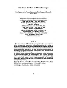
(2) For x2 > y2 one may infer −α − a2 < a1 < β + a2 whereas − α+β < a2 < 0, 2 (3) If x2 < y2 then in similar to previous possibility we obtain −α + a2 < a1 < β − a2 and 0 < a2 < α+β , 2 whereas −∞ < a0 , a3 < ∞ in all three cases. Considering all of these results we conclude that −∞ < a0 , a3 < ∞, −α+ | a2 |< a1 < β− | a2 | and 0 ≤| a2 |
0 these results can be interpreted as −α < a1 − a2 < a1 + a2 and a1 − a2 < a1 +a2 < β which in together combined into −α < a1 −a2 < a1 + a2 < β, Hence the result.

FOURIER TRANSFORM

9

Now we are ready to define the Fourier transform for bicomplex variable. 3.2. Definition. Let f (t) be a real-valued continuous function in (−∞, ∞) that satisfies the estimates (5). The Fourier transform of f (t) can be defined as Z ∞ ˆ exp(i1 ωt)f (t)dt, ω ∈ C2 . (9) f (ω) = F{f (t)} = −∞

The Fourier transform fˆ(ω) exists and holomorphic for all ω ∈ Ω where Ω (given in (8)) is the region of absolute convergence of fˆ. 3.3. Existence of Fourier transform. Theorem: If f (t) be a real valued function and is continuous for −∞ < t < ∞ satisfying estimates (5) then fˆ(ω) (defined in (9)) exists in the region (8).

Proof: fˆ(ω) =

Z

∞

exp(i1 ωt)f (t)dt Z−∞ ∞

=

Z

∞

exp(i1 ω1 t)f (t)dt.e1 + −∞

exp(i1 ω2 t)f (t)dt.e2 −∞

Both the integrals exist when −α < Im (ω1 = x1 + i1 x2 ) < β and −α < Im (ω2 = y1 + i1 y2 ) < β. So fˆ(ω) exists for ω = ω1 e1 + ω2 e2 = a0 + i1 a1 + i2 a2 + i1 i2 a3 where −∞ < a0 , a3 < ∞, −α+ | a2 |< a1 < β− | a2 |, and 0 ≤| a2 |
0 then F{f (at)} = −∞ exp(i1 ωt)f (at)dt = R 1 ∞ exp(i1 ωa u)f (u)du = a1 fˆ( ωa ) where we take at = u. a −∞ R ∞If a < 0 then for a =R ∞−b : b > 0 we have F{f (at)} = exp(i1 ωt)f (at)dt = −∞ exp(i1 ωt)f (−bt)dt. Now taking −∞ bt =R −u the integral is R∞ −∞ ω ω − 1b ∞ exp(i1 −b u)f (u)du = 1b −∞ exp(i1 −b u)f (u)du R ∞ 1 ω 1 ˆ ω = −a −∞ exp(i1 a u)f (u)du = −a f ( a ). 1 ˆ ω f ( a ). From above these results we conclude F{f (at)} = |a| (4) Convolution theorem Theorem: The Fourier transform of the convolution of two functions f (t) and g(t),−∞ < t < ∞ is the product of their Fourier transforms, respectively fˆ(ω) and gˆ(ω) i.e.

Z

∞

F {f (t) ∗ g(t)} = F

 f (u)g(t − u)du = fˆ(ω)ˆ g (ω).

−∞

Proof: By definition

= = + = +

−∞

(10)

∞

 f (u)g(t − u)du F {f (t) ∗ g(t)} = F −∞  Z ∞ Z ∞ exp(i1 ωt) f (u)g(t − u)du dt −∞ −∞ Z ∞  Z ∞ exp(i1 ω1 t) f (u)g(t − u)du dt.e1 −∞ −∞ Z ∞  Z ∞ exp(i1 ω2 t) f (u)g(t − u)du dt.e2 −∞ −∞ Z ∞  Z ∞ f (u) exp(i1 ω1 t)g(t − u)dt du.e1 −∞ −∞ Z ∞  Z ∞ f (u) exp(i1 ω2 t)g(t − u)dt du.e2 Z

−∞

12

BANERJEE, DATTA AND HOQUE

using method for changing order of integrals in complex analysis [30] Z ∞  Z ∞ f (u) exp(i1 ωt)g(t − u)dt du = −∞ −∞ Z ∞ f (u) exp(i1 ωu)ˆ g (ω)du, using shifting property (see property 2) = −∞  Z ∞ f (u) exp(i1 ωu)du gˆ(ω) = fˆ(ω)ˆ g (ω). = −∞

(5) Theorem: If f (t) and tr f (t), r = 1, 2, ...., n are all integrable in −∞ < t < ∞ then

F {tn f (t)} = (−i1 )n

dn ˆ {f (ω)} dω n

where fˆ(ω) is the Fourier transform of f (t). Proof: We will prove this theorem by using the method of mathematical induction and differentiation under integral sign. For n = 1,

= =

= = =

d ˆ ∂ ˆ ∂ ˆ f (ω) = f1 (ω1 )e1 + f2 (ω2 )e2 dω ∂ω1 ∂ω2 Z ∞ Z ∞ ∂ ∂ exp(i1 ω1 t)f (t)dt.e1 + exp(i1 ω2 t)f (t)dt.e2 ∂ω1 −∞ ∂ω2 −∞ Z ∞ Z ∞ ∂ ∂ {exp(i1 ω1 t)f (t)}dt.e1 + {exp(i1 ω2 t)f (t)}dt.e2 −∞ ∂ω1 −∞ ∂ω2 using Leibnitz rule in complex analysis [30] Z ∞ Z ∞ i1 tf (t) exp(i1 ω1 t)dt.e1 + i1 tf (t) exp(i1 ω2 t)dt.e2 −∞ −∞ Z ∞ i1 tf (t){exp(i1 ω1 t)e1 + exp(i1 ω2 t)e2 }dt −∞ Z ∞ i1 tf (t) exp(i1 ωt)dt = i1 F{tf (t)} −∞

⇒ F{tf (t)} = −i1

d ˆ f (ω). dω

FOURIER TRANSFORM

= = =

= = =

13

Now for n = 2, in similar to the case for n = 1,   d2 ˆ d d ˆ f (ω) = f (ω) dω 2 dω dω Z ∞  d i1 tf (t) exp(i1 ωt)dt dω −∞ Z ∞ Z ∞ ∂ ∂ exp(i1 ω1 t)tf (t)dt.e1 + i1 exp(i1 ω2 t)tf (t)dt.e2 i1 ∂ω1 −∞ ∂ω2 −∞ Z ∞ Z ∞ ∂ ∂ i1 {exp(i1 ω1 t)tf (t)}dt.e1 + i1 {exp(i1 ω2 t)tf (t)}dt.e2 −∞ ∂ω1 −∞ ∂ω2 using Leibnitz rule [30] Z ∞ Z ∞ 2 − t f (t) exp(i1 ω1 t)dt.e1 − t2 f (t) exp(i1 ω2 t)dt.e2 −∞ Z−∞ ∞ − t2 f (t){exp(i1 ω1 t)e1 + exp(i1 ω2 t)e2 }dt Z−∞ ∞ t2 f (t) exp(i1 ωt)dt = −F{t2 f (t)} − −∞

d2 d2 ⇒ F t2 f (t) = − 2 fˆ(ω) = (−i1 )2 2 fˆ(ω). dω dω 

Proceeding in this way we obtain F {tn f (t)} = (−i1 )n

dn ˆ f (ω). dω n

(6) Theorem: If f (t) and f (r) (t), r = 1, 2, ...., n are piecewise smooth and tend to 0 as | t |→ ∞, and f with its derivatives of order up to n are integrable in −∞ < t < ∞ then F{f (n) (t)} = (−i1 ω)n fˆ(ω)} r

where fˆ(ω) is the Fourier transform of f (t) and f (r) (t) = dtd r f (t). Proof: We will prove it also using method of induction. For n = 1, Z ∞ 0 F{f (t)} = exp(i1 ωt)f 0 (t)dt −∞ Z ∞ ∞ = [f (t) exp(i1 ωt)]−∞ − i1 ω exp(i1 ωt)f (t)dt −∞

= 0 − i1 ω fˆ(ω) = −i1 ω fˆ(ω).

14

BANERJEE, DATTA AND HOQUE

Similarly for n = 2, Z

∞

exp(i1 ωt)f 00 (t)dt −∞ Z ∞ ∞ 0 = [f (t) exp(i1 ωt)]−∞ − i1 ω exp(i1 ωt)f 0 (t)dt 00

F{f (t)} =

0

−∞ 2ˆ

= 0 − i1 ωF{f (t)} = (−i1 ω) f (ω). Proceeding with similar arguments we can get F{f (n) (t)} = (−i1 ω)n fˆ(ω)}. • Corollary If f (t) is finite, i.e. f (t) = 0 | t |> T and continuous inside | t |≤ T , then its complex Fourier transform is an entire function. RT As it’s consequence fˆ1 (ω1 ) = −T exp(i1 ω1 t)f (t)dt and fˆ2 (ω2 ) = RT exp(i1 ω2 t)f (t)dt. So the bicomplex Fourier transform fˆ(ω) −T exists and converges absolutely within the whole C2 . 3.6. Examples. (1) If f (t) = exp(−a | t |), a > 0 then it satisfies estimates (5) for α = β = a and its complex Fourier transforms are 2a 2a ˆ2 (ω2 ) = fˆ1 (ω1 ) = 2 , f . a + ω1 2 a2 + ω2 2 Both fˆ1 , fˆ2 are holomorphic in the strip −a < Im (ω1 ), Im (ω2 ) < a. Then the bicomplex Fourier transform will be 2a fˆ(ω) = 2 a + ω2 with region of convergence Ω = {ω = a0 +i1 a1 +i2 a2 +i1 i2 a3 ∈ C2 :

0 ≤| a2 |< a,

−a+ | a2 |< a1 < a− | a2 |}.

(2) If 

exp(−t), t > 0; 0, t≤0 then α = 1 but β be any positive number. Here 1 fˆ(ω) = 1 − i1 ω and its region of convergence is 1+β Ω = {ω = a0 +i1 a1 +i2 a2 +i1 i2 a3 ∈ C2 : 0 ≤| a2 |< , a1 > −1, for any positive β}. 2 f (t) =

FOURIER TRANSFORM 2 (3) If f (t) = exp(− t2 ) then fˆ(ω) = of convergence is

√

15 2

2π exp(− ω2 ) and its region

Ω = {ω = a0 + i1 a1 + i2 a2 + i1 i2 a3 ∈ C2 : −∞ < a1 , a2 < ∞}. (4) If 

1, | t |≤ a; 0, | t |> a then its complex Fourier transforms in both ω1 and ω2 planes are entire functions. Then using the corollary we obtain fˆ1 (ω1 ) = 2 sin(aω1 ) and fˆ2 (ω2 ) = ω22 sin(aω2 ), where the singularity at ω1 ω = 0 is removable. In this case the bicomplex Fourier transform will be fˆ(ω) = ω2 sin(aω) and it’s region of convergence is C2 . (5) If  0, t < 0; f (t) = exp(− Tt ) sin(ω0 t), t ≥ 0, T, ω0 > 0 f (t) =

which might represent the displacement of a damped harmonic oscillator. Here from the estimates (5) we have α = T1 . Then complex Fourier transform in ω1 (similar for ω2 ) plane is given by   1 1 1 fˆ1 (ω1 ) = − 2 ω1 − ω0 + iT1 ω1 + ω0 + iT1 which is holomorphic in in the infinite strip Im (ω1 ) > − T1 except Re (ω1 ) 6= ±ω0 . In this problem the bicomplex Fourier transform will be   1 1 1 fˆ(ω) = − 2 ω + ω0 + iT1 ω − ω0 + iT1 with region of convergence 1 Ω = {ω = a0 +i1 a1 +i2 a2 +i1 i2 a3 ∈ C2 : a0 6= 0, ±ω0 ; a3 6= 0, ±ω0 ; a1 > − } T where a = Im (ω2 )− Im (ω1 ) : Im (ω ), Im (ω ) > − 1 . 2

2

1

2

T

4. Conclusion In this paper we have exploited the bicomplex version of Fourier transform method and the condition of absolute convergence of the transformed bicomplex-valued function. We examine the usual properties of Fourier transform in the ring of bicomplex numbers. Finally

16

BANERJEE, DATTA AND HOQUE

let us point out that in our observation the concepts introduced or results obtained in this work are the generalization of the corresponding concepts or results in complex analysis. References [1] [2] [3] [4] [5] [6] [7] [8] [9] [10] [11] [12] [13] [14] [15] [16] [17] [18] [19] [20] [21] [22] [23] [24] [25] [26] [27] [28] [29] [30]

C.Segre, Math.Ann. : 40, 1892, pp:413. N.Spampinato, Atti Reale Accad. Naz. Lincei,Rend.: 22, 1935, pp:38. N.Spampinato, Ann.Mat.Pura.Appl.: 14, 1936, pp:305. W.R.Hamilton, Lectures on quaternion Dublin:Hodges and Smith: 1853. G.B.Price, Marcel,Dekkar: 1991. S.Olariu, Norh-Holland Mathematics Studies,Elsevier: 190,2002,pp:269. G.Shpilker, Doklady AN SSSR: 282,1985,pp:1090. G.Shpilker, Doklady AN SSSR: 293,1987,pp:578. S.Dimiev,R.Lazov,S.Slavova, Topics in Contemporary Differential Geometry,Complex Analysis and Mathematical physics: 2006,pp:50-56. I.M.Yaglom, Academic Press, N.Y.: 1968. I.M.Yaglom, Springer, N.Y.: 1979. K.S.Charak, D.Rochon,N.Sharma, Fractals: 17,2009. R.Goyal, Tokyo Journal of Mathematics:30,2007. S.Gal, Nova Science Publishers: 2002. A.Motter,M.Rosa, Adv. Appl. Clifford Algebra: 8,1998,pp:109. J.Ryan, Complex variables,Theory and Applications: 1,1982,pp:119. R.K.Srivastava, Proc.Soc.of Special Functions and their applications (SSFA): 2005,pp:55. S.R¨ onn, arXiv:math/0101200[math.CV],2001. Y.Xuegang, Adv.Appl.Clifford Algebra: 9,1998,pp:109. V.Kravchenko,M.Shapiro, Pitman Research Notes in Math.,Addison-WesleyLongman: 351,1996. D.Dart,D.Haag,H.Cartarins, J.Main, G.Wunner arXiv:1306.3871[quantph],2013. D.Rochon,S.Tremblay, Adv.Appl.Clifford Algebra: 14,2004,pp:231. D.Rochon,S.Tremblay, Adv.Appl.Clifford Algebra: 16,2006,pp:135. E.Martineau,D.Rochon, Int. J. Bifurcation Chaos: 15,2005. A.Kumar,P.Kumar, International Journal of Engineering and Technology: 3,2011,pp:225. A.Banerjee,S.K.Datta,A.Hoque, Mathematical Inverse Problems:1,2014. S.Bochner, K.Chandrasekharan, Princeton University Press: 1949. G.Kaiser, Birkhauser: 1994. Y.V.Sidorov, M.V.Fedoryuk, M.I.Shabunin, Mir Publishers,Moscow: 1985. J.H.Mathews, R.W.Howell, Narosa Publication : 2006.

FOURIER TRANSFORM

17

A Banerjee, Department of Mathematics, Krishnath College, Berhampore, Murshidabad 742101, India S K Datta, Department of Mathematics, University of Kalyani, Nadia 741235, India Md. A Hoque, Gobargara High Madrasa (H.S.),Hariharpara, Murshidabad 742166, India

18

BANERJEE, DATTA AND HOQUE

Appendix

a2 a1+a2=β (0, β)

a1+a2=-α

a1-a2=-α

(0,α)

a1-a2=β

=

(-α,0)

(β,0)

a1

(0,-α)

(0, -β)

𝑎1 − 𝑎2 plane in the concerned region of convergence Fig-1