Standard branching process theory implies that the probabilities of eventual .... Figure S1: Dependence of the optimal mutation rate µopt on the number of lethal ..... Achieving a low mutation rate can be costly (resources used to maintain repair.
Evolutionary invasion and escape in the presence of deleterious mutations 1
Claude Loverdo 1
1,2
and James O. Lloyd-Smith
Department of Ecology and Evolutionary Biology, University of California, Los Angeles, CA 90095, USA 2
Fogarty International Center, National Institutes of Health, Bethesda, MD 20892, USA
Appendices S1 General model S1.1
The limit of small mutation rates µ
For a given mutation rate mutate to another strain
k
and initial strain
as
p0,k (µ).
lethal mutants, into immediate neighbors strain
0,
and all other neighbors
j
0,
we de�ne the probability to
We divide the other strains, including
i
that are one mutation away from
that are further away.
We assume that
the mutation rates at all sites are proportional to each other, so that in the limit of low mutation rates,
p0,j = Ω(µ2 )
p0,i = µr0,i
with
r0,i
a proportionality factor and
or smaller; then we can de�ne the probability that replication
2 i r0,i µ + Ω(µ ) function starting from one replicator of strain 0 is:
occurs without mutation,
p0,0 = 1 −
P
+ ....
The generating
X X R0 1 g0 (~z) = + z0 p0,0 z0 + p0,i zi + p0,j zj . R0 + 1 R0 + 1 i j
(1)
Standard branching process theory implies that the probabilities of eventual
i ei are the smallest positive gk (e1 , ..., en ) = ek (and the survival probaof strain i is si = 1 − ei ) [1]. This leads to
extinction starting from one replicator of strain solution of the system of equations bility starting from one replicator
the following equation for the survival probabilities:
0 = s0 − R0 (1 − s0 ) p0,0 s0 +
X i
1
p0,i si +
X j
p0,j sj .
(2)
We di�erentiate with respect to
µ:
0 =∂µ s0 + R0 ∂µ s0 p0,0 s0 +
X
p0,i si +
i
X
p0,j sj
j
− R0 (1 − s0 ) s0 ∂µ p0,0 +
X
si ∂µ p0,i +
X
i
j
X
X
sj ∂µ p0,j
(3)
− R0 (1 − s0 ) p0,0 ∂µ s0 +
p0,i ∂µ si +
i
p0,j ∂µ sj .
j
µ = 0. Without mutations, p0,0 (µ = 0) = 1 p0,k6=0 (µ = 0) = 0. For immediate mutational neighbors, ∂µ p0,i |µ=0 = r0,i . 2 Because p0,j = Ω(µ ) or smaller, therefore ∂µ p0,j = Ω(µ) or smaller, and so ∂µ p0,j |µ=0 = 0. Denoting x b as the value of x when µ = 0, ! X X d 0 = ∂d r0,i sb0 + r0,i sbi − R0 (1 − sb0 )∂d µ s0 + R0 ∂µ s0 sb0 − R0 (1 − sb0 ) − µ s0 . We now evaluate the expression for and
i
i (4)
This can be simpli�ed to yield:
∂d µ s0 = If
R0 < 1, sb0 = 0,
R0 (1 − sb0 ) X r0,i (sbi − sb0 ). 1 − R0 + 2R0 sb0 i
and:
R0 X r0,i sbi + Ω(µ2 ). 1 − R0 i
s0 = µ If
(5)
R0 > 1, sb0 = 1 − 1/R0 ,
(6)
and:
1 µ X s0 = 1 − r0,i (sbi − sb0 ) + Ω(µ2 ). + R0 R0 − 1 i
(7)
The sign of this derivative summarizes whether a small amount of mutation leads to a higher survival probability than no mutation. In both cases, this sign is determined by the sign of
P
i r0,i (sbi
− sb0 ),
i.e. mutations are bene�cial if the
weighted average of the survival probabilities of the neighboring mutants in the absence of mutations is larger than the survival probability of the initial strain without mutations. This criterion is su�cient for the mutations to be bene�cial.
S1.2
Approximations for lethal mutations
One can notice that in equation (1) of the main text, the probability that there is no lethal mutation is per replication is
U (µL
(1 − µ)L .
If the mean number of lethal mutations
in our notation), then often in the literature (see for
example [2]) the probability that there is no lethal mutation is taken as
exp(−U ).
This is the probability to have zero mutations for a Poissonian distribution, implying that there can be any number of lethal mutations, whereas in our model there could be at most small,
(1 − µ)L ' exp(−µL),
L
lethal mutations. However, in practice, for
µ
and this approximation is sometimes used in the
following calculations.
2
S1.3
Iterative approximations for survival probabilities
The survival probabilities are the solutions of:
0 = s1 − R1 (1 − s1 )(1 − µ)L ((1 − µ)s1 + µs2 ) and the analogous expression for
2
in the equation).
1 ↔ 2
(8)
(i.e. interchanging the indices
1
and
We derive approximate solutions by iteration, including
successively more steps of mutation. The �rst step is the survival probability with only lethal mutations, solution of
0 = si − Ri (1 − si )si (1 − µ)L : (0)
si If we replace
(0)
s2 by s2
� � Ri (1 − µ)L − 1 . = max 0, Ri (1 − µ)L
in the analogous of equation (8) for
s1 ,
then a quadratic equation for of
(0)
s2
(9)
1 ↔ 2, this equation is (1) s1 as a function
that we can solve to obtain
, using the additional property that survival probabilities are positive.
Recursively, the higher-order solutions follow with:
(k+1) si
with
1 = 2Ri (1 − µ)L+1
� � q (k) 2 2 2L+1 µRi sj , αi + αi + 4(1 − µ) (k)
αi = −1 + Ri (1 − µ)L (1 − µ − µsj ),
with
(i, j) = (1, 2)
or
(10)
(2, 1).
S1.4
Further approximations in the regime of evolutionary escape (R1 < 1, R2 > 1) � (0) (1) L L+1 When R1 < 1, R1 (1−µ) < 1, thus s1 = 0, leading to s2 = max 0, 1 − 1/(R2 (1 − µ) ) . (1) We de�ne se2 = 1 − 1/(R2 (1 − µ)L+1 ). This expression makes intuitive sense, because in this parameter regime, the strain 1 is similar to an additional lethal
(1)
s2
(0)
s2 but with L + 1 instead of L. (1) opt L+1 When µ is close to µ , it can be shown that R2 (1−µ) > 1, thus s2 = se2 (1) .
mutant neighbor for strain 2, so
is like
This leads to:
1 s1 ' 2R1 (1 − µ)L+1
� � q 2 (1) 2 2L+1 α f1 + α f1 + 4(1 − µ) µR1 se2 ,
α f1 = −1 + R1 (1 − µ)L (1 − µ − µse2 (1) ). (1) Then, we assume µse2 � 1 − R1 (1 − µ)L+1 , leading mation for s1 : R1 µ(R2 (1 − µ)L+1 − 1) . s1 ' R2 (1 − µ)(1 − R1 (1 − µ)L+1 )
(11)
with
to a general approxi-
(12)
We can now optimize the approximate survival probability to learn about
µopt .
µ equals zero when: � � 0 = 1 − R1 (1 − µ)L+1 1 − R2 (1 − µ)L+1 + µ(L + 1)(1 − µ)L+1 (R2 − R1 ). The derivative of (12) with respect to
(13) We further assume that
exp(−µ(L + 1)).
µ � 1,
leading to
(1 − µ)L+1 = exp(ln(1 − µ)(L + 1)) '
The equation to solve is
0 = 1 − R1 e−X
�
� 1 − R2 e−X + Xe−X (R2 − R1 ), 3
(14)
opt Figure S1: Dependence of the optimal mutation rate µ on the number of lethal mutations and the �tnesses of the two viable strains, and comparison of the approximations. The two columns show the same data with linear scale on the left and log scale on the right (except for the top left panel where only the y-axis is linear). Different solutions are denoted with di�erent line styles, as follows: exact solution (red solid line), from se1 (2) (purple dashed line), with a development in µse2 (1) (13) (blue dotted line), and with the additional (1 − µ)L+1 ' exp(−µ(L + 1)) (14) (green dotdashed line). The bottom row shows two additional approximations: the development in R2 → 1+ (15) (black dotted line), and the development in R2 large (16) (black solid line). Unless indicated otherwise, L = 10, R1 = 2/3 and R2 = 9.
X = µ(L + 1). In this regime, as the equation to solve is function of X and µ and L independently, µopt ∝ 1/(L + 1). As expected, the more numerous
with not
the lethal mutants, the riskier mutations become, and the smaller the optimal mutation rate.
4
Regime R2 − 1 � 1
In the limit
R2 = 1 + �, µ(L + 1) = Ω(�),
to:
µopt →
Regime R2 � 1
In the limit
R2
and (14) leads
R2 − 1 . 2(L + 1)
(15)
large, (14) can be simpli�ed as:
X = 1 − R1 e−X .
(16)
This equation can only be solved numerically, but importantly it shows that the result does not depend on
R2 .
Comparison of the approximations
Figure S1 shows the comparison of the
se1 (2) gives a good approximation except (1) L+1 for L small. The development in µse2 (13) and the further step (1 − µ) ' exp(−µ(L + 1)) (14) �t well provided 1 − R1 is not too close to 0. The bottom approximations with the exact solution.
panels show that the solutions of (15) and (16) are good approximations in their intended regimes.
S2 Di�erent numbers of lethal mutations Here we discuss how
µopt
is in�uenced by di�erent values of
ing the analysis to the regime where
R1 < 1
and
L1
and
L2 , restrict-
R2 > 1.
General equations are the same as for the simple model, except that strain i has
Li
lethal neighbors. By analogy with (10), our starting point is:
(2)
s1 =
1 1 1 − 2 R1 (1 − µ)L1 +1
v u u 4µs(1) 2 − +t + 1−µ 1−µ (1) µs2
1−
(1) µs2
1 − R1 (1 − µ)L1 +1 1−µ (17)
(1) with s2 When
L2 +1
= 1 − 1/(R2 (1 − µ) 1 − R1 is not very
).
small compared to 1,
(1)
µs2
is small compared to
(2) the other terms, and the development of s1 leads to:
s1 '
R1 µ(1 − µ)L1 R2 (1 − µ)L2 +1 − 1 . 1 − R1 (1 − µ)L1 +1 R2 (1 − µ)L2 +1
which di�erentiated with respect to optimal mutation rate:
µ
(18)
leads to the following equations for the
L1 +1 −R
0 = 1+(L2 −L1 )µ−R1 (1+µ(L2 +1))(1−µ)
2 (1−µ(L1 +1))(1−µ)
L2 +1 +R
1 R2 (1−µ)
L1 +L2 +2 .
(19)
We con�rm that if
L1 = L2 = L,
we recover (13).
(1−µ)Li +1 by exp(−µ(Li +1)) Xi = µ(Li + 1), yielding the equation
As for the simple model, we can approximate in the limit to solve for
Li � 1. µopt :
Once again we set
1 + X2 − X1 − R1 (1 + X2 )e−X1 − R2 (1 − X1 )e−X2 + R1 R2 e−(X1 +X2 ) = 0. In the limit
R1 e−X1 ' 0.
L1 � L2 ,
we have
Similarly in the limit
(20)
X1 � X2 and so (20) simpli�es to 1 − X1 − L2 � L1 , (20) simpli�es to 1+X2 −R2 e−X2 ' 5
!2
,
R1 = 0.5, R2 = 1.5
R1 = 0.5, R2 = 10
R1 = 0.9, R2 = 10
Value of µopt as a function of L1 and L2 (y axis), for the exact solution (solid red lines) and approximations s(2) (17) (purple dashed lines), development in 1 (1) µs2 small (19) (blue dotted lines), further approximation of L1 and L2 large (20) (green dot-dashed lines), and more extreme approximation (21) (black straight lines).
Figure S2:
0.
Therefore, in the regimes where one strain is threatened by many more lethal
mutations than the other, it is the optimization on this strain which determines
µopt ,
independent of the parameters of the less threatened strain.
As an extreme approximation, we can consider the optimal mutation rate as
6
a piecewise combination of these two cases:
µopt ' min
��
� � �� X1 X2 −X1 −X2 1 − X − R e = 0 , 1 + X − R e = 0 . 1 1 2 2 L1 + 1 L2 + 1 (21)
Figure S2 shows how the exact numerical solution for
µopt
compares to a
L1 and L2 . Values of µopt calculated (2) numerically from s1 (17) work well except when L1 and L2 are both very small; (1) those calculated from the approximations for µs2 small, (19) and (20), work series of approximations, as a function of
well if
1 − R1
is not too small. The rough approximation (21) works remarkably
well in the limit
L1
and
L2
large, especially if one of them is much larger than
the other.
S3 Two steps towards a �tter mutant In the case of two binary loci, described in the text:
g00 =
�� � R00 � 1 L L 2 2 + 1 − (1 − µ) + (1 − µ) (1 − µ) z00 + µ(1 − µ)z01 + µ(1 − µ)z10 + µ z11 1 + R00 1 + R00 (22)
leading to the equation for the survival probability:
s00 = R00 (1 − s00 )(1 − µ)L ((1 − µ)2 s00 + µ(1 − µ)s01 + µ(1 − µ)s10 + µ2 s11 )
(23)
and analogous equations for the other strains. Our analysis focuses on the case where both sites must mutate in order for the virus to attain a higher �tness (sometimes called a �jackpot model�). That is, we take
R00 = R01 = R10 = R1
and
R11 = R2 .
In this case we have the set
of equations:
s0 = R1 (1 − s0 )(1 − µ)L ((1 − µ)2 s0 + 2µ(1 − µ)s1 + µ2 s2 ), s1 = R1 (1 − s1 )(1 − µ)L (((1 − µ)2 + µ2 )s1 + µ(1 − µ)s0 + µ(1 − µ)s2 ) and L
2
2
s2 = R2 (1 − s2 )(1 − µ) ((1 − µ) s2 + 2µ(1 − µ)s1 + µ s0 ).
(24) (25) (26)
These equations are solved numerically to build �gure 4 of main text. Analogous calculations and conclusions can be made when more mutations are needed, and show the generality of the qualitative �ndings from the 2-step case (�gure S3).
S4 Deleterious mutations When all deleterious mutations are strictly lethal
When all deleterious
mutations are strictly lethal, the survival probabilities are found from the system of equations:
s1 = R1 (1 − s1 )(1 − µ)L ((1 − µ)s1 + µs2 ), and the symmetric equation for
1 ↔ 2.
7
(27)
s(0)
íííííííí íííí í ã ã ã í ã ã ãì ã í éì éì éì ãì éì ã éì éì ã 0.030 í í é é ííãì ã éì ã éì í ã éì ã éì éì éì ã éì ã é í é íì ã í éì í ã é í 0.025 í ã ãé èèèèèèèèèèèè ì ì í ã ã é í ì ã é ì íì è ì èèè ã é ì 0.020í í ã ã é é è ì è ã ì é ã ì è ì í è é ã ã é ì é è 0.015ì ã ì é è ì ã é í ã é ì é ã è è ì 0.010ì è éè í è ã é ì ã è è è 0.005 éè ì è è è 0.01 0.02 0.03 0.04 0.05
s(0,0)
s(0,0,0) 0.0030ì è è éèí 0.0025 ã ã éã í 0.0020ì ã í éããã ííí 0.0015ì ééããã ííííí ííííí éé ããéãéãéãéãéãéãéãéããí ì í ãéì éééì éì 0.0010ìì ì ì ì éì ì ì ì ì ì ãéì éã ã éãì ã éì ãé ì éì í ì ìì ì ãé í ì ãé í ãé ì 0.0005 èèèèèèèèèèèè è ì è ì í ãé ì è è è í ãé ì èèèèèè è í ãé è èèèèè 0.00 0.01 0.02 0.03 0.04 0.05
s(0,1)
or
s(1,0)
0.008 ã è í ã ííí íííí 0.006 ãã íííí ãã ããããããí íííí ã ã ãéì ã ã éì í éì éì éì ã éì éì éì é ã é éãããããã ã ì éì éì ã éì é ã ì éì ã éì é í éì ì 0.004 éééì ã é í ì ééì éì ã é é í ì ì ì ì è è è è è ã è è é í è è ì è ì è è ì ã é èèèèè è ì 0.002 è ì í ã é èè è è í ã é ì è è èèèèè 0.00 0.01 0.02 0.03 0.04 0.05
íííííííí 0.030 íííí í í ã ã ã ã ã í ã ã éì éì éì ã éì éì í ã éì ã éì éì í ã éì ã éì íãì ã éì í éì ã í éì éì í ã éì ã éì ã í é é í 0.025 í ì ã í ã é ì é ì ã í è è è è ì ã è é íì èèèèè èèèèè í 0.020í é ãì ã é é ì è ì ã ã èè ì é ã í è ì ì é ã é ã ì é è 0.015ì ã ì é è ì ã í é ã é ì ã é è è 0.010ì í è éè ã é ì ì ã è è è í ã é ì 0.005 éè è è ì è è è
s(0,0,1) , s(0,1,0)
s(1,0,1) , s(0,1,1)
or
s(1,0,0)
0.008 ã è ãí í 0.006 ãã íííí íííí ã íííí éãããããããããã ã ã ã ã íííí ãì ãì ãì éì éì éì éì éì é ã é éì ã é éì ã é éì ã 0.004 ééì éì ã éì éì ã éì ã éì é í ì éééì é ã é í ì ì ì ì ã é í ì èèèèèèèèèèèèèè è ì ã é 0.002ì è ì èè í è ì ã é èè è í ã é ì è èèè í ã é ì è è è 0.00 0.01 0.02 0.03 0.04 0.05
0.01 0.02 0.03 0.04 0.05
or
s(1,1,0)
è 0.030 ííííííííííí í ãã ã í ã ã í ã ã í éì éì éì éì ãì éì í éì í ã ã é éì ã éì í í éì ãì éì í ã é ã 0.025 í éì í ã í éì éì ã í éì ì ã éì ã é éã ì ã í éã í ã ì é 0.020íì ã ã é èèèèèèèèèèè ì è é ì è ã è é ãé í ì èè ã ã è ì é ì é ã è 0.015 ì ì é ã è ì é í è ã ã ì é é ì è ã é è è 0.010ì í è ã é ì é è è ì ãè í ã é ì è è 0.005 éè è ì í ã é ì è è è è 0.00 0.01 0.02 0.03 0.04 0.05
Survival probability as a function of the mutation rate, when one, two or three sites must mutate in order to increase �tness (i.e. a jackpot-like landscape, with �tness R1 for all strains except the adapted one which has R2 ). The three rows of panels show the results for a 1-step, 2-step and 3-step path to adaptation, from top to bottom. R2 = 9, L = 10. Figure S3:
When one deleterious mutation leads to a reduced �tness Rd , and two or more deleterious mutations are lethal In the case when one deleterious mutation leads to a reduced �tness to
R0 = 0
Rd ,
and two or more deleterious mutations
(lethal), the system is:
s1 = R1 (1−s1 )(1−µ)L−1 ((1−µ)2 s1 +(1−µ)µs2 +Lµ(1−µ)s1d +Lµ2 s2d ),
(28)
s1d = Rd (1−s1d )(1−µ)L−1 ((1−µ)2 s1d +(1−µ)µs2d +µ(1−µ)s1 +µ2 s2 ),
(29)
and symmetric equations for
1 ↔ 2.
When any non-zero number of deleterious mutations leads to a reduced �tness Rd , or when deleterious e�ects are multiplicative For the two other cases shown in �gure 5 of the article, with bility starting from a replicator with allele
j
sj,i
the survival proba-
at the adaptive site and
i
mutated
deleterious sites, the system is:
s1,i = R1,i (1−s1,i )
� � i � � L−i X i X L − i p+q µ (1−µ)L−p−q ((1−µ)s1,i+q−p +µs2,i+q−p ), p q q=0 p=0 (30)
1 ↔ 2, with sj,0 = Rj . For the case of a uniform Rj,i>0 = Rd , and for the case of multiplicative e�ects
and symmetric equations for deleterious e�ect, we set we set
Rj,i = Rj αi . 8
S5 Within-host viral dynamics S5.1
Generating function
1 − qi , a virion of strain i does not successfully infect a host (1 − qi )zi0 in the generating function). When a cell is successfully infected (probability qi ), it generates o�spring virions according to a geometric distribution with mean Ni (generating function 1/(1 + Ni (1 − z))), each of L 0 0 which can be independently mutated (z = (1 − (1 − µ) )zi zj (lethal mutants) L+1 L +(1 − µ) zi (no mutation) +(1 − µ) µzj (mutation at the adaptive site but
With probability cell (term in
no lethal mutation)). The generating function starting from one virion of strain 1 is then:
g1 (z1 , z2 ) = 1 − q1 +
q1 . 1 + N1 (1 − µ)L (1 − (1 − µ)z1 − µz2 )
(31)
The corresponding equations for the survival probabilities are:
0 = s1 − (q1 − s1 )N1 (1 − µ)L ((1 − µ)s1 + µs2 ), and the analogue with
(32)
1 ↔ 2.
The iterative approximations start with:
(0) si
�
�
= max 0, qi
1 1− Ri (1 − µ)L
�� (33)
and proceed according to:
(k+1) si
v 2 u (k) (k) u 4µq s(k) µsj µsj i j 1 1 1 u − +t + qi − − = qi − . 2 Ni (1 − µ)L+1 1−µ 1−µ Ni (1 − µ)L+1 1−µ (34)
S5.2
No change in the dependence of survival probability on mutation rate when qi and Ni are adjusted with Ri constant
Let us de�ne
si = si (q1 , N1 , q2 , N2 ), s0i = si (rq1 , N1 /r, rq2 , N2 /r)
and
Using equation (32),
sei = s0i /r.
N1 (1 − µ)L ((1 − µ)s01 + µs02 ), r
(35)
0 = rse1 − r(q1 − se1 )N1 (1 − µ)L ((1 − µ)se1 + µse2 ).
(36)
0 = s01 − (rq1 − s01 ) which can be rewritten as:
Thus
sei
and
si
both satisfy the equations for survival probabilities for this
(0, 1] × (0, 1] si (rq1 , N1 /r, rq2 , N2 /r) = rsi (q1 , N1 , q2 , N2 ).
system. Because there is at most one solution of these equations in [1], we have shown that
S5.3 We use
Approximations in the regime of evolutionary escape (R1 < 1, R2 > 1) (2)
s1
as an approximation, with
(1)
s2 = q2 (1 − 1/(R2 (1 − µ)L+1 )).
When
studying the optimum numerically, we observe that there are two regimes:
q2
and
q1 � q2 . 9
q1 >
The optimal mutation rate for the model of within-host viral infection as a function of R2 − 1, 1 − R1 and L, comparing the approximations in the two parameter regimes. Each subpanel shows results for two sets of parameters q1 and q2 . In the regime where q1 > q2 (q1 = 10−3 , q2 = 10−4 ), the exact solution (black dashed line) is represented along with the approximations s(2) (34) (blue up triangles and blue solid 1 line) and approximation µs(1) small (13) (green squares and green solid line). In the 2 regime where q1 � q2 (q1 = 10−5 , q2 = 10−1 ), the exact solution (black solid line) is represented along with the approximations s(2) (34) (purple down triangles and 1 purple dashed line), q1 small (40) (red dotted line), and the further approximation (41) (orange dot-dashed line). Figure S4:
Regime q1 > q2
1 − R1 is not (1) s2 scales as q2 ,
We can proceed as in the simple model: when
(1) (2) too small, we develop s1 assuming µs2 small (for �xed R2 , so the smaller q2 , the better this approximation), and obtain: (1)
(1 − µ)L µN1 q1 s2 (1 − µ)L µR1 q2 s1 ' = 1 − (1 − µ)L+1 N1 q1 1 − (1 − µ)L+1 R1 10
�
1 1− R2 (1 − µ)L+1
� .
(37)
When di�erentiated with respect to
µ,
it leads to the following equation for
µopt : 0 = 1 − R1 (1 − µ)L+1
� 1 − R2 (1 − µ)L+1 + µ(L + 1)(1 − µ)L+1 (R2 − R1 ),
�
(38) which is the same as (13) for the simple model. Therefore the conclusions are the same as for the simple model.
Regime q1 � q2
(2)
s1
Developing
� s1 ' q1
in the limit
q1
small, we obtain:
R2 (1 − µ)q1 1+ µq2 R1 (1 − (1 − µ)L+1 R2 )
which di�erentiated with respect to
µ
� ,
(39)
is proportional to:
−1 + (1 − µ)L+1 R2 (1 − (L + 1)µ).
(40)
µ = µopt , we obtain a good R2 − 1 � 1, then µL � 1, thus (40) leads to opt the limit R2 � 1, (40) leads to µ ' 1/(L + 1).
By assuming that this expression equals zero when approximation (�gure S4).
If
µopt ' (R2 − 1)/(2(L + 1)).
In
These limiting expressions can be combined in:
µopt ' which, though only rigorous for for most of the
R2
R2 − 1 , (L + 1)(R2 + 1)
(41)
R2 −1 � 1 and R2 � 1 is a good approximation
range (�gure S4).
S6 Repetitively changing environment Achieving a low mutation rate can be costly (resources used to maintain repair mechanisms, replication slowed by proofreading steps, etc.) [3, 4, 5, 6]. In the following discussion, we completely neglect this aspect, focus only on the impact of the mutations on �tness, how the interplay between adaptive mutations and deleterious load a�ects survival.
Adding a cost to �delity would increase the
optimal mutation rate. We study evolutionary invasion and escape, which is adaptation to environmental change. In the main text, we focus on one step of environmental change. In this section we discuss the case of several successive environmental changes. There are three di�erent relevant time-scales: the time ronmental changes, the time change, and the time
τm � τa ,
τm
τa
τe
between 2 envi-
to adapt via mutations to an environmental
for the mutation rate to change. It is possible to have
for example when one or a few mutations are needed to adapt to the
environment whereas many mutations are needed to modify the mutation rate. Then there are three situations:
•
If
τe � τa ,
then environmental changes are too rapid for genetic changes
to be a relevant response.
•
If
τe � τm ,
then mutation rates are selected to be low when the envi-
ronment is stable; when the environment changes, mutants with higher mutation rates are most likely to produce adaptive mutations, and will hitch-hike to high frequency with these mutations, but will decline again when the environment stabilizes [7].
11
•
If
τa � τe � τm ,
the mutation rate will evolve towards an optimum
between limiting the deleterious load but allowing for adaptation when the environment changes. We focus on this regime. Let us assume that replicators face successive environments environment
I , the best reproducing genotype is i.
I = 1, 2, 3,... In τe is long
Let us assume that
enough that before a new environmental change, the population is limited in its growth (for example by resource availability) and has reached the mutation-
pj,I−1 of replicators j in environment I − 1 j = i − 1 (and decreases for increasing mutation rates), and of the order of µ or smaller for all the other replicators (and increasing with the mutation rate). Let us assume that an average of NI replicators are passed from the environment I − 1 to I . NI could be a constant, for example a �xed carrying capacity for environment I − 1, or the size of a founder population that has migrated from environment I − 1 to environment I . If NI is constant, dNI /dµ = 0. If NI depends on the replicator �tness, then at the mutation-selection balance, NI decreases with increasing mutation rates, i.e. dNI /dµ < 0. Let us assume that the number of replicators passed to the next environment follows a Poisson distribution. We de�ne sj,I as the probability of survival of a lineage initiated by one replicator of strain j in environment I . Q The survival probability through all the environmental changes is s = I sI , with sI the survival probability for one step of environmental change from I − 1 to I . If there are kj replicators of strain j passed to the new environment I , Q kj the survival probability is 1 − j (1 − sj,I ) . We assume that the survival probabilities of all replicators are independent, and consequently the average sI selection balance. The proportion
is of the order of one for the replicator
is:
sI = 1−
YX j
(1−sj,I )kj
kj
Y (NI pj,I−1 )kj exp(−NI pj,I−1 ) = 1− exp(−NI pj,I−1 sj,I ). kj ! j (42)
To infer which e�ects are predominant, we study how
s
varies with the
mutation rate:
X 1 dsI ds =s , (43) dµ sI dµ I Q � X X � dNI ds dpj,I−1 dsj,I j exp(−NI pj,I−1 sj,I ) Q =s pj,I−1 sj,I + NI sj,I + NI pj,I−1 , dµ 1 − j exp(−NI pj,I−1 sj,I ) j dµ dµ dµ I
X (1 − sI ) X ds =s dµ sI j
�
I
dNI dpj,I−1 dsj,I pj,I−1 sj,I + NI sj,I + NI pj,I−1 dµ dµ dµ
(44) � . (45)
Because of the factor
(1 − sI )/sI ,
the steps that will matter more are the steps
with the smallest survival probability, which are the limiting steps. We discuss below which factors are the most important for a given step of environmental change.
There are many possible scenarios for
NI .
depends on the �tnesses of the population of replicators in environment
dNI /dµ < 0, and lower mutation rates are where NI does not depend on the overall
12
If NI I − 1,
favored. We will focus on the case �tness, or weakly, so that we can
neglect the terms proportional to compare the terms
•
For any
sj,I dpj,I−1 /dµ
j 6= i, dsj,I /dµ
for speci�c cases.
µ, except pj6=(i−1),I−1 � pi−1,I−1 . Consequently, for likely that pj,I−1 dsj,I /dµ is much smaller than is expected to depend strongly on
it is
dsi,I /dµ to be small, and as pi,I−1 � pi−1,I−1 , then pi,I−1 dsi,I /dµ is much smaller than pi−1,I−1 dsi−1,I /dµ.
We expect that
•
we only need to
Besides,
any j 6= i or i − 1, pi−1,I−1 dsi−1,I /dµ.
•
dNI /dµ. In this scenario, pj,I−1 dsj,I /dµ.
and
it is likely
As the replicator of strain i − 1 is the most abundant in environment P P dpj,I−1 ' I − 1, dpi−1,I−1 /dµ ' − j6=(i−1) dpj,I−1 /dµ. Thus j sj,I dµ P dpj,I−1 j6=(i−1) (sj,I − si−1,I ) dµ . As i is the �ttest strain in environment I , sj6=i,I < si,I . In most cases, sj6=i,I � si,I , which guarantees (si,I − dp to be the most important of the sum. This term is positive: si−1,I ) i,I−1 dµ when the mutation rate increases, there are more pre-existing mutants i in the environment I − 1 which will be adaptive to the new environment I.
pi−1,I−1 dsi−1,I /dµ pi−1,I−1 is of the order of one minus corrections propor-
Thus the two terms that are the most likely to be signi�cant are and
(si,I −si−1,I )
dpi,I−1 dµ .
dpi,I−1 is also about dµ one. For values of µ for which si−1,I varies strongly, pi−1,I−1 dsi−1,I /dµ will dominate. In the article, we maximize the survival probability analogous to si−1,I . dpi,I−1 opt,1step Where µ is close to µ as calculated for one step, (si,I − si−1,I ) dµ will be important, and overall will shift the rate maximizing survival to values opt,1step somewhat larger than µ . tional to the mutation rate. If all mutation rates are similar,
To summarize, successive environmental changes (occurring faster than the time required for the mutation rate to evolve) will select for a mutation rate close to the optimal mutation rate we have calculated for one step (taking the step with the smallest survival probability, with the strain most adapted to previous environment as the initial replicator).
A more detailed model is necessary to
calculate corrections, due to the number of replicators passed from the previous environment (which decreases the optimal mutation rate) and the number of pre-existing mutants (which acts in the opposite way).
References [1] Harris TE. The theory of branching processes. Dover phoenix editions; 1963. [2] Bull JJ.
2008. The optimal burst of mutation to create a phenotype.
Theor. Biol..
254,667�73.
J.
[3] Sniegowski PD, Gerrish PJ, Johnson T, Shaver A. 2000. The evolution of mutation rates: separating causes from consequences. BioEssays.
22,1057�
66. [4] Furió V, Moya A, Sanjuán R.
2005. The cost of replication �delity in an
RNA virus. Proc. Natl. Acad. Sci. USA.
13
102,10233�7.
[5] Thébaud G, Chadoeuf J, Morelli MJ, McCauley JW, Haydon DT.
2010.
The relationship between mutation frequency and replication strategy in positive-sense single-stranded RNA viruses. Proc. R. Soc. B. [6] Regoes R, Hamblin S, Tanaka M.
277,809�17.
2013. Viral mutation rates: modelling
the roles of within-host viral dynamics and the trade-o� between replication �delity and speed. Proc. R. Soc. B.
280,20122047.
[7] Denamur E, Matic I. 2006. Evolution of mutation rates in bacteria. Mol. Microbiol.
60,820�7.
14