Apple Defect Detection and Quality Classification with MLP-Neural Networks Devrim UNAY, Bernard GOSSELIN TCTS Laboratory, Faculte Polytechnique de Mons Initialis Scientific Park, 1, Copernic Avenue B-7000 Mons Belgium Phone : +32 (0)65 37 47 45 Fax : +32 (0)65 37 47 29 E-mail:
[email protected] Abstract- The initial analysis of a quality classification system for ‘Jonagold’ and ‘Golden Delicious’ apples is shown. Color, texture and wavelet features are extracted from the apple images. Principal components analysis was applied on the extracted features and some preliminary performance tests were done with single and multi layer perceptrons. Keywords- computer vision; image processing; defect segmentation; feature selection; neural networks
I. INTRODUCTION Accurate automatic classification of agricultural products is a necessity for agricultural marketing to increase the speed and minimize the miss-classifications. The European Union defines three quality classes (“extra”, “I”, and “II”) for the fresh apples with the tolerances of 5, 10, and 10 per cent by number or weight of apples, respectively [1]. The apples in the “extra” class must be of superior quality with no defects or irregularity in shape, whereas the classes “I” and “II” can contain defects up to 1 and 2.5 cm2, respectively. Also, Belgian Trade Practices define four classes for ‘Golden Delicious’ apples with respect to the ground color of the fruit (‘++’ for the greenest, ‘+’, ‘’, and ‘r’ for yellow). It is clear that the classification of different kinds of apples into predetermined categories as accurate and quickly as possible is a hard task. Many researchers have made considerable efforts in the field of machine vision based classification of apples. Several approaches like monochrome-colorednear infrared imaging, and local-global methods have been tried. Zion et al [2] introduced a computerized method to detect the bruises of Jonathan, Golden Delicious, and Hermon apples from magnetic resonance images by
threshold technique. The algorithm was only able to discriminate between all-bruised and non-bruised apples and was not applicable to on-line detection. Pla and Juste [3] presented a thinning algorithm to discriminate between stem and body of the apples on monochromatic images. However the task of classifying the calyx and defected parts real-time was missing. Yang and Marchant [4] used the ‘flooding’ algorithm for initial segmentation and ‘snakes’ algorithm for refining the boundary of the blemishes on the monochromatic images of apples. They applied both median and gaussian filters to remove impulsive noise and smooth small features. Nakano [5], studied color (red, green, and blue) grading of “San Fuji” apples by two types of neural network. First one classified the pixels into six categories with an overall accuracy of over 95 per cent, but mistook the injured surfaces as vines. The second one classified the fruit into five categories with the recognition rate of 75 per cent for damaged fruits. However, the recognition rate of class A was not higher than 33 per cent. Miller et al [6] compared different neural network models for detection of blemishes of various kinds of apples by their reflectance characteristics and concluded that multi-layer back propagation (MLBP) method gave the best recognition rates. Also they found that increased complexity of the neural network system did not yield to better results. Leemans [7], segmented defects of ‘Golden Delicious’ apples by a pixel-wise comparison method between the chromatic (rgb) values of the related pixel and the color reference model. The local and global approaches of comparison were effective, but further research was needed. In his second research [8], Leemans used a Bayesian classification method for pixel-wise segmentation on chromatic images of ‘Jonagold’ apples. The method failed in discriminating between pixels of transition area and russet.
Wen and Tao [9] introduced automated rule-based system by near-infrared images to classify ‘Red Delicious’ apples as defected or not. They reached a speed of 50 apples per second with high recognition rates, but had problems in identification of stem/calyx. Because of the concavity of the apple, the intensity of the light decreases from the center to the boundaries. Penman [10], introduced an array of blue light sources and an algorithm to correctly discriminate apple blemishes from stem, calyx and their concavities. However, the algorithm has to be improved in accuracy, implemented in real time and used in conjunction with defect detection algorithms. In the field of machine vision based classification, scientists have used many other kinds of agricultural products other than apples. Kim et al [11] experimented on kiwi fruits. Guyer and Yang [12] used genetic artificial neural networks to classify cherries. Diaz et al [13] introduced an algorithm to classify olives. Laykin et al [14], used image processing techniques to classify tomatoes. Patel et al [15] developed an expert sorting system for eggs. Brezmes et al [16] classified peaches and pears. Harel and Smith [17] used a texture-based approach to classify grapes. II. METHODOLOGY The acquisition system used in this study to retrieve the apple images was the same with Leemans’ [7]. A colored camera with a frame grabber, were used to acquire the images while the apples were passing through a tunnel providing diffuse light. Data set was composed of 229 images (22 bruised, 207 defected) of ‘Jonagold’ apples and 76 images (12 bruised, 64 defected) of ‘Golden Delicious’ apples. The images contained various kinds of defects, like russet, scab, fungi attack, bitter pit, bruising, punches, insect holes and growth defects, as well as stem and calyx areas. However, the initial analysis presented here includes a small group of this data set. A. Initial Processing During the acquisition of images orientation and rotation of the apples were neither controlled nor fixed. Therefore, background had to be excluded from each image. The images of bruised apples of each kind contained a bi-colored (gray, black) background, whereas the defected ones were imaged on black background only. Low pass filter at level 150 on Bchannel and band-pass filter at levels 35-225 on
channels R-G were applied to eliminate gray and black backgrounds, respectively. Dimensions of the images were differing within the data set. In order to decrease computation time while doing mathematical operations, images had to be square. So, areas outside the apple were deleted and the remaining images were resized to 128x128 dimension by nearest neighborhood method. B. Feature extraction ‘The problem of classification is basically one of partitioning the feature space into regions, one region for each category.’ [18] So, high discriminating features will lead to high and accurate classification rates. Color values (RGB-channels), as local features, are directly related with the images, so they were introduced to the system without any change. For the classification of a pixel, neighboring pixels can provide vital evidence. So, two groups of color features were introduced to the system; oneto-one pixel mapping of color feature set in the first, whereas n-to-one in the other, with n (or neighborhood) determined by the rgb-window size. Structural analysis will yield important information for classification, so co-occurrence matrix of Haralick et al [19] is used to extract textural features. Co-occurrence matrix is a single level dependence matrix that contains the relative frequencies of two coordinate elements separated by a distance d. As you move from one pixel to another on the image, entries of the initial and final pixels become the coordinates of the co-occurrence matrix to be incremented, which in the end will represent structural characteristics of the image. Therefore, moving in different directions and distances on the image will lead to different co-occurrence matrices. In literature, most commonly used pixel separation distance and directions (angles) are 1 pixel and 0, π/4, π/2, and 3π/4 radians, respectively [20, 21], which are also used in this study. The four textural features derived from the co-occurrence matrices are: 1. Energy 255 255
f 1 (d ) = ∑∑ s(i, j , d )
2
i = 0 j =0
2. Entropy 255 255
f 2 (d ) = ∑∑ s(i, j , d ) ⋅ log s (i, j , d ) i =0 j =0
3. Inertia 255 255
f 3 (d ) = ∑∑ (i − j ) ⋅ s(i, j, d ) i =0 j =0
2
4. Local Homogeneity 255 255
1 ⋅ s(i, j, d ) 2 j = 0 1 + (i − j )
f 4 (d ) = ∑∑ i =0
In the above equations, s(i, j, d ) refers to the normalized entry of the co-occurrence matrices found by dividing the initial entries with total number of pixels of the sub-image, where (i, j ) are the coordinates of the co-occurrence matrices and d is the pixel separation distance. In order to locate the spectral differences within and between images, many of the spectral analysis methods like Fourier, wavelet or cosine transforms could be used. The advantage of localization in time and frequency made wavelets preferable. Within the orthogonal and compactly supported wavelets (daubechies, symlets, and coiflets), coiflets have more number of vanishing moments at the same order, so have more information on the details. Therefore, 2nd order coiflets wavelet decomposition is applied on each sub-image retrieving 1 approximate and 2x3 detailed (horizontal, vertical and diagonal for each order) coefficients. Calculating the texture and wavelet features of the whole image will yield important global results maybe, but obviously will not provide us enough information about both the size and type of the defects that are crucial in classification or discrimination between stem, calyx and defected areas. Because of that, these features were calculated on windowed sub-sections of each image. Two different window approaches were used to get the sub-images. In discrete window approach, images were divided into 64 16x16 non-overlapping subimages. On each sub-image, both textural and wavelet features were calculated and they were related to each pixel within that sub-image. However in sliding approach, features were calculated a pixel at a time on the 16x16 neighborhood by zero-padding the areas outside the image. That’s why sliding window method required 256 times more computation than discrete window for 128x128 image size and 16x16 window size, which is undesirable for an automatic process. Initial analysis showed that B-channel provided very little information of classification compared to R and G channels, so the texture and wavelet features were calculated on the R and G channels of the images only. The resulting four texture features of a pixel were from the average of co-occurrence matrices in all directions.
Wavelet features were found by taking the average and standard deviations of the coefficients of each decomposition class. At the end of feature extraction, there were 8 textural, 28 wavelet and 3 color features (27 for 3x3, or 75 for 5x5 rgb-windows) making a total of 39 (63, or 111) features. C. Feature selection In order to get high performance of classification, the features introduced to any neural network system should be in the same range, which can be achieved by normalization. The features are normalized so that the mean is 0 and the standard deviation is 1 by the formula:
f i′ =
[ f i − µ ( f i )] σ ( fi )
where f i & f i′ are the initial and final values of a feature, respectively, µ ( f i ) is the mean and σ ( f i ) is the standard deviation of all the values of the class that feature belongs to. “The designer usually believes that each feature is useful for at least some of the discriminations.” [18] However, superfluous and class-conditionally dependent features may lead to terrible classification performance. So, principal components analysis was applied on the features to get an uncorrelated data set. First covariance matrix of the feature set was calculated and then the matrix of the eigenvectors of this covariance matrix was multiplied with the feature set, producing transformed feature set whose components are uncorrelated and ordered according to the magnitude of their variance. Then the components, which contribute only a small amount (1 per cent in this case) to the total variance in the transformed feature set, are eliminated. D. Neural Network model As the literature review indicates there are few researches in this field done with neural networks, which are used in this work. The true power and advantage of neural networks lies in their ability to represent both linear and nonlinear relationships and to learn these relationships directly from the data being modeled. The neural network in this study is composed of perceptron neurons with an adaptive supervised learning back-propagation algorithm. E. Manual Segmentation of Apples Segmentation of apple images into determined classes was done manually by an image processing software. One of the images of ‘Golden Delicious’ apples and its segmentation into four classes is shown below (Figures 1, 2).
Figure 1: Original image (Gold001.tif)
Class
Pixel #
Ratio %
Background
3520
21.48
Healthy skin
9355
57.10
Defected skin
3048
18.60
Stem/Calyx
461
2.81
Table 1: Pixel class-distribution of Gold001.tif
18 more apple images containing both defected and stem/calyx areas were segmented like the above making a total of 19 images (8 of ‘Golden Delicious’ and 11 of ‘Jonagold’) for the current data set. The following results are obtained analyzing these images. III. RESULTS & DISCUSSION A. Three-Class SLP Test The background pixels in the images can be separated from the apple region by simple image processing techniques. So, without the background, a pixel-wise three-class classification test can be done on the current data set. For each image, 37 pixels (samples) selected homogeneously from each three classes were homogeneously mixed and introduced to the system for training. Then for the validation set, same approach was used to select samples from the rest of the image. As a
rgb-wind 1x1
90.19 92.75 67.53 72.51 39.15 29.59
3x3
90.80 92.03 68.19 72.81 44.36 32.96
5x5
90.61 93.03 66.11 70.04 51.05 35.45
1x1
89.38 89.33 66.66 71.03 47.00 33.02
3x3
93.46 92.22 67.87 72.17 52.48 34.40
5x5
92.03 93.08 66.97 70.86 55.26 36.36
sliding
The original images were 128x128 in dimension with three-color channels (rgb). In Figure 2, resulting images are binary and the segmented pixels are the areas white in color. The difference between the sizes of the original and segmented images is due to visual preference of the authors; i.e. there was no alteration in dimensions. Table 1 represents the class-distribution of the pixels of the segmented image.
wind discrete
Figure 2: Segmentation into four-classes (left-to-right: background, healthy skin, defected, stem/calyx)
result, the training and validation sets were composed of 111 samples. Three different rgb-window sizes (1x1, 3x3, and 5x5) and two different window types (discrete and sliding) were used to extract color features and texture, wavelet features, respectively. Normalization and principal components analysis were applied on all the feature sets by the schemes explained before. ‘Train with one, test with rest’ method was used for the simulations of 19 images with a single layer perceptron neural network. The average results of all 19 simulations are in Table 2. tr
vl
rec
c1
c2
c3
Table 2: Three-class simulation results of ‘train with one, test with rest’ method.
The above results are all in percentages. ‘c1, c2, c3’ in the first row represents the classes healthy, stem/calyx and defected, respectively. Recognition rates of each method on training and validation data sets are over 90 per cent (except ‘sliding’ window, ‘1x1’ rgb-window method), whereas the validation rates are between 65-70 per cent. The training and validation sets include same number of samples from each class, but simulation sets are composed of all the pixels of the images and the average distribution of the images is 1.5, 9.5, and 89.0 per cent for stem/calyx, defected and healthy classes, respectively. This unequal distribution results in the difference between the validation and recognition rates. ‘Sliding window’ method provides more information to the system than the ‘discrete’ one, by definition. Although there is no significant difference in the overall recognition rates, recognition rates of the stem/calyx (‘c2’) and defected (‘c3’) classes show this increase in performance. As the size of the ‘rgb-window’ is increased, performance of the system should increase also. It is observable in the ‘c2’, ‘c3’ classes. The effects of different methods on the performance of the system are obvious, but the class recognition rates are lower than the standards, which courage the authors to continue on testing with increased size and dispersion of the training and validation sample sets. The reader should also be aware that more information introduced to the system will improve the performance with an increase in the computation times of not
only the recognition but also the feature extraction and selection parts of the system. B. Three-Class MLP Test The results of the three-class single layer (SLP) test encouraged the authors to make tests with multi layer perceptrons. According to its performances in the previous test, one of the images (Gold002.tif from ‘Golden Delicious’ apples) was selected for this test. The method was again ‘train with one, test with rest’ in order to compare the results with single layer ones. 1 and 2 hidden layers with 0, 50, 100, 150, and 200 neurons were used in the system. wind
rgbwind system
rec
c1
c2
c3
discrete sliding
1x1
0-0
65.98 70.65 68.83 22.10
3x3
0-0
61.10 65.10 84.69 20.39
5x5
0-0
68.53 73.32 85.29 21.40
1x1
0-0
63.74 64.69 41.31 58.24
3x3
0-0
65.95 66.16 56.58 65.42
5x5
0-0
56.16 56.36 72.65 51.90
Table 3: SLP results of Gold002.tif. rgbwind
discrete
1x1
200-200 65.45 66.30 51.51 59.62
3x3
200-50
66.52 66.09 63.96 70.96
5x5
100-50
67.10 67.03 69.85 67.38
1x1
150-50
69.58 69.00 39.76 79.39
3x3
200-0
68.99 68.89 65.24 70.56
5x5
150-50
67.80 67.15 70.34 73.45
sliding
wind
system
rec
c1
c2
c3
Table 4: Best MLP results of Gold002.tif.
C. Three-Class Homogeneous Sampling Test In the previous tests, the system trained with one of the apple images was expected to accurately recognize the rest of the apples. It will be more realistic if a group of samples from each apple variety (‘Golden Delicious’ and ‘Jonagold’) is introduced to the system as the training set. Samples selected homogeneously will yield more realistic results about the population. For this reason all the 19 images segmented (11 ‘Jonagold’ and 8 ‘Golden Delicious’) were distributed evenly within the training, validation and simulation sets as 7 (5 ‘Jonagold’ - 2 ‘Golden’), 6 (3-3) and 6 (3-3), respectively. To enable a comparison with the previous tests, the sample size selected from each class of each image was 37, making a total of 777 samples for training, 666 samples for validation and all samples of the simulation images for simulation. Discrete windowing and 3x3 rgbwindow methods were used for feature extraction. The important problem at this point is ‘Which image should be in which data set?’ or ‘Which samples provide more information of discrimination about the population?’ A method of random selection of images for each data set can be a solution. 100 random selections were done and these sample sets were used to feed the single layer neural network. The average rates of these 100 tests were 73.38, 67.84, 76.94, 82.26, 64.75, and 35.77 per cent for recognition of training, validation, simulation, healthy, stem/calyx and defected sets, respectively. Table 5 displays the results of this method with the results of three-class SLP test for comparison, where the abbreviations ‘1,8’ (train with one, test with rest), ‘7,6,6’ (homogeneous sampling), ‘A’ (average) and ‘B’ (best) are used. test
The recognition rates found for multi layer perceptron network with different number of neurons were promising. The best performances are displayed in Table 4. An interesting observation is that, the recognition rates of multi layer network are higher than those of the single layer one (Table 3) for defected class (‘c3’). A careful reader will notice that as the system gets more complex, recognition rates of defected class increase with a decrease in the recognition of healthy or stem/calyx classes. Hence, there is a compromise between the recognition rates of each class independent of the complexity of the system. This explains the constancy of the overall recognitions even though the system complexity changes.
1,8 7,6,6
tr
vl
rec
c1
c2
c3
A
90.80
92.03
68.19
72.81
44.36
32.96
B
85.59
85.59
75.73
81.06
67.26
31.54
A
73.38
67.84
76.94
82.26
64.75
35.77
B
67.05
60.36
89.89
90.45
62.23
83.69
Table 5: Results of ‘1,8’ and ‘7,6,6’ tests.
The rows indicated as ‘A’ in Table 5, represent the averaged results of all combinations of ‘1,8’ and ‘7,6,6’ (19 combinations for ‘1,8’ and 100 combinations for ‘7,6,6’), while ‘B’ indicated rows show the results of best classifying combination in each test. In the training step, the population (19 images) was represented by 7 images in ‘7,6,6’ test, which was 1 for ‘1,8’ test. The effect of this different sampling can be observed in the results of average simulation rates. They are strictly higher for test ‘7,6,6’ than those of ‘1,8’. The best
recognition rates for ‘7,6,6,’ are very promising with 90 and 83 per cent for healthy and defected classes, respectively. However, even for the best case of ‘7,6,6’ class-recognition rates found are quite low with respect to the standards.
3.
IV. CONCLUSION & FUTURE WORK The field of automatic classification of agricultural products is increasingly attracting the attention of researchers as well as governments and agricultural markets. However, an accurate automatic classification system for apples requires highly detailed research due to the difficulty of the task and high number of parameters affecting the performance. Although the classification approaches used in the literature (image-based or apple-based) are different than the pixel-based one of this study, the comparison of the best homogeneous sampling result with the ones achieved by other authors can guide the reader for better judgment. Nakano [5] reached over 75 per cent recognition rates for about 40 defected apples with his neural network B, whereas our best results were 89.9 and 83.7 per cent for overall and defected pixels of 6 defected images. Also, Wen et al [9] reached about 84 per cent recognition for over 300 stem and calyx images, which is nearly 62 per cent for our case. The preliminary results shown here are promising, but not enough. There is a lot more to do. More samples of the population should be introduced to the training set, better discriminating features (local or global) should be searched, the affects of different feature selection algorithms (like Fisher’s linear discriminator) on the performance should be compared, improvements of combined methods like statistical analysis and neural networks should be examined, performance of the system should be verified in real-time and in real environment…
6.
V. ACKNOWLEDGEMENTS This project is known as the CAPA (Classification Automatique de Produits Agricoles) project and is funded by Ministere de la Region Wallonne, Belgium. VI. REFERENCE 1.
UN/ECE Standard on apples and pears http://www.unece.org/trade/agr/welcome.htm then select Standards/Fresh fruit and vegetables 2. Zion B., et al, “Detection of bruises in magnetic resonance images of apples”, Comp. Elec. Agric., 13, 289-299, 1995.
4. 5.
7. 8. 9. 10. 11. 12. 13. 14. 15. 16. 17. 18. 19. 20.
21.
Pla F., Juste F., “A thinning-based algorithm to characterize fruit stems from profile images”, Comp. Elec. Agric., 13, 301314, 1995. Yang Q., Marchant J. A., “Accurate blemish detection with active contour models”, Comp. Elec. Agric., 14, 77-89, 1996. Nakano K., “Application of neural networks to the color grading of apples”, Comp. Elec. Agric., 18, 105-116, 1998. Miller W. M., et al, “Pattern recognition models for spectral reflectance evaluation of apple blemishes”, Postharvest Bio. Tech., 14n 11-20, 1998. Leemans V., et al, “Defects segmentation on ‘Golden Delicious’ apples by using color machine vision”, Comp. Elec. Agric., 20, 117-130, 1998. Leemans V., et al, “Defect segmentation on ‘Jonagold’ apples using color machine vision and a Bayesian classification method”, Comp. Elec. Agric., 23, 43-53, 1999. Wen Z., Tao Y., “Building a rule-based machine-vision system for defect inspection on apple sorting and packing lines”, Expert Sys. App., 16, 307-313, 1999. Penman D. W., “Determination of stem and calyx location on apples using automatic visual inspection”, Comp. Elec. Agric., 33, 7-18, 2001. Kim J., et al, “Linear and non-linear pattern recognition models for classification of fruit from visible-near infrared spectra”, Chemo. Intel. Lab. Sys., 51, 201-216, 2001. Guyer D., Yang X., “Use of genetic artificial neural networks and spectral imaging for defect detection on cherries”, Comp. Elec. Agric., 29, 179-194, 2000. Diaz R., et al, “The application of a fast algorithm for the classification of olives by machine vision”, Food Res. Int., 33, 305-309, 2000. Laykin S., et al, “Development of a quality sorting machine using machine vision and impact”, ASAE An. Int. Meet., paper no: 99-3144, July 18-21, Toronto, Canada, 1999. Patel V. C., et al, “Development and evaluation of an expert system for egg sorting”, Comp. Elec. Agric., 20, 97-116,1998. Brezmes J., et al, “Fruit ripeness monitoring using an Electronic Nose”, Sensors and Actuators., B 69, 223-229,2000. Harel N. K., Smith T. E., “A texture based approach” http://www.cc.gatech.edu/classes/cs7321_97_winter/participant s/smith/fp/final.html Pattern Classification and Scene Analysis, Duda R. O., Hart P. E., Wiley & Sons, Canada, 1973. Haralick R. M., et al, “Textural features for image classification”, IEEE Trans. SMC, 3, 610-621, 1973. Latif-Ahmet A., et al, “An efficient method for texture defect detection: sub-band domain co-occurrence matrices”, Image Vision Comp.,18, 543-553, 2000. “Epileptic activity detection in EEG with Neural Networks”, Varsta M. et al, research report B3, Comp. Eng. Lab., Helsinki Univ. Tech., Finland, April 1997.