DEFECT DETECTION AND CLASSIFICATION IN NONWOVEN WEB IMAGES USING NEURAL NETWORK Maryam Yousefzadeh 1 , Pedram Payvandy 2 Seyyed Ali Seyyedsalehi 3 & Masud Latifi 4 1, 2
PhD student, Textile Engineering Department email:
[email protected] email:
[email protected] 3 Assistant Professor, Biomedical Engineering Department email:
[email protected] 4 Professor, Textile Engineering Department email:
[email protected] Amirkabir university of Technology, Hafez Ave., Opposite of Somayyeh, Tehran, IRAN Phone: +98 (021) 64542636 , fax: +98 (021) 66400245
Abstract In the last 25 years the amount of textile nonwoven used for industrial and commercial applications increased more than 10 times. Consequently quality control is became one of the basic issues in textile industry. Analysis of texture content in digital images plays an important role in the automated visual inspection of nonwoven web images to detect their defects and classify them. However, there is a lack of special method for robust quality control and monitoring during production of nonwoven. This paper presents a new method for defect detection in nonwoven images using the fractal dimension for feature extraction and neural network back propagation algorithms for defects classification. The results of proposed methodology are illustrated in defective nonwoven web images where the defective are recognized and classified with more than 99.5% accuracy. Key Words: nonwoven – defect detection – fractal dimension – neural network image analysis
1
Introduction
Visual inspection constitutes an important part of quality control in industry. Quality control is designed to ensure that defective products are not allowed to reach the customer. For this reason, monitoring of products characteristics and appearance during of production is very important. Until recent years, this job has been heavily relied upon human inspectors. But today all of the manufacturing plants go toward the automated quality control systems. This fact comes into consideration in textile and nonwoven industries. Nonwoven is one of the new
branches in textile industry that in the last 25 years the amount of textile nonwoven used for industrial and commercial applications increased more than 10 times. A large variety of industrial products, ranging from carpet to baby napkins, make use of nonwoven. For all these products, the fabric quality plays an important role. It is deteriorated by in-homogeneities such as thick and thin spots and neps. Because of the importance of the nonwoven appearances and also the undesirable influences of non uniformity in nonwoven webs, and economical detriment that follow it, on-line quality control and monitoring is become very important. Development of fast and specialized equipment, however, has facilitated the application of image processing algorithms to real-world industrial inspection problems. Industrial vision systems must operate in real-time, produce a low false alarm rate and be flexible to accommodate variations in inspection sites. Automated visual inspection of web materials is very complex task and the research in this field is widely open (Brzakovic & Vujovic 1996). Many attempts have been made to solve these problems. Norton-Wayne et al.(1992) describe a simple system, based on adaptive threshold and binary filtering. An optical system for real time defect detection is shown in paper of Olsson and Gruber (1993). It is based on light scattering and uses electro-optical equipment for defect detection. Dar et al. (1997) present a system for detecting one type of defect (pilling) in the five grades. The Radon transform is used for feature extraction and fuzzy logic is implemented for rating. Escofet et al. (1996) analyse a variety of defects in different fabrics and in every case, the flaws are finally segmented from the background, while Gabor functions are used for feature extraction. Mueller and Nickolay (1994) use the morphological image processing for gray-level inspections. The system of Huart and Postaire (1994) has use multi-cameras with associated hardware. Group of researches in Georgia institute of technology (1997) implement the wavelets transform and fuzzy logic to solve this task. Stojanovic and et al. (1999) describe simple system, based on fast binary algorithm to determine possible defect regions and use neural network to classify the defect. Campbell in 1997 present 2D Discrete Fourier Transform to feature extraction and feed forward neural network to classification. Pakkanen & et al. (2004) use the MPEG-7 standard feature descriptor and evolving tree self organizing map for defect image classification. Ahmet (2000) use cooccurrence matrix for feature extraction and defect inspection. Serdaroglu & et al. (2004) use wavelet packet transform to feature extraction of images and Euclidean distance for defect detective. Karras & et al. (1998) present the feature extraction method which is based on wavelets transform, SVD analysis, and co-occurrence matrix. Sezer & et al. (2003) have implemented independent component analysis (ICA) for feature extraction. In present paper the fractal dimension of non woven images are calculated for feature extraction. After that, an artificial neural network, trained by using a back-propagation algorithm, is implemented for defect detection and classification. Using numbers of the possible defect classes, the system gives consistent and repeatable results in the experimental and real industrial implementations.
2 2.1
Theories and image analysis algorithms Fractal Geometry and Dimension
In 1623, Galileo expressed that the book of nature was written in mathematic languages and the alphabets of this language is triangles, circles and other geometrical shapes, that human being could not understand it carefully (Peitgen & Richter 1986). The Euclidean geometry is the axiomatic study of lines, circles and triangles that shaped form an ideal, therefore approximate basis for understanding geography, mechanics and every real thing. From this perspective, nature is like noisy mathematics and crumpled slightly out of focus. Fractal create an
alternative to Euclidean geometry whose elements are not lines and circles but iterations and self-similarities, whose surface are not smooth but jogged, whose feature are not perfect but broken. Fractal is a new geometry that enables us to understand formerly inexplicable real world phenomena. Fractal provides insight into the distribution of galaxies, the shape of coastlines and growth of crystals (Frame & Mandelbrot 2002). In nature, we can see more fractal object such as fern, cauliflowers, clouds, trees and so on. The fractal objects have distinctive boundaries that occupied the constant volume or space. Fractal dimension can define any changing in the details of object. Until now, many fractal dimensions were introduced with special applications (Mandelbrot 1983). The fractal dimension is changed between 0 to 3 and takes a real amount. For curve, this varies between one up to two and for surface changes from two to three. The fractal dimension shows freedom’s degree of object. From the perspective of some application and also the concept that is used in present research, fractal dimensions can be used instead of human vision in some systems. So using this concept, it is very useful for object’s pattern investigation. Some of the most important and useful of fractal dimensions are box counting, compass and self-similar dimension.
2.1.1
Box counting Dimension
Box counting dimension used in many applications in different systems. It is related to selfsimilarity structures, but it can be applied even to the random structure without a conspicuous self-similar unit, like a coastline. For determining box counting dimension ( D B ) it is assumed that the object is covered by a square mesh of various sizes “ s ” and then number of boxes ( N (s) ) contain part of the image (containing the object) is counted. Because N is the function of the mesh size, N (s) increases as s decreases. The box counting dimension ( DB ) is given by the slope of the linear portion of a log( N (s ) ) vs. log(1 / s ) graph as expressed by Equation 1. log N ( s) = DB log(1 / s )
2.1.2
(1)
Compass Dimension
The compass dimension is a relationship between the compass divider setting and measured length. To measure the length of the random fractal curve, a compass divider must divide by a compass divider or ruler with certain ruler setting. If multiplying the ruler length by the number of rulers that is needed to cover the object’s image length, the approximate length of a curve can be expressed as Equation 2:
L =N ´l
(2)
By decreasing the length of rulers, the more accurate length of the curve can be obtained, because of the closer measurement to the path of the curve. So if we plot ln ( L ) against ln (l ) for a range value of l , the slope will be an estimation for the compass dimension ( DC ) (Bourke 1983). ln ( L ) = ln (l )1- DC + c¢
2.2
(3)
Neural Network
In recent years intensive development of artificial intelligence (AI) methods has been observed, leading to the design of computer expert systems to perform the tasks previously carried out by a man. From among many methods of AI, artificial neural networks (ANNs) can be used to
construct computer systems, which can replace human experts. They can create the basis for an inference mechanism as effective as deterministic formulas based on classic two-dimensional logic. The advantage of ANNs over classic algorithmic methods lies in the fact that, with the classic methods, it is necessary to know the full model of a procedure, which would enable a deterministic rule of inference to be formulated. On the other hand, ANNs are ‘self-programming’, i.e. they can design a program using the data fed into the system. ANNs can process the information, and perform such tasks as: ♦ Matching defected or retrieved input with the closest pattern stored, ♦ Matching two patterns, diagnosis, analysis, ♦ Classification, i.e. dividing the input into classes or categories, ♦ Recognition, that is to say, input classification, even though the input corresponds with no patterns stored, etc. ANNs have found application in many fields of science, including textile and clothing industry.
2.2.1
Neural Network Training: Back-Propagation Algorithm
The back-propagation algorithm, perhaps the most utilized of existing neural network algorithms, gets its name from the way it handles errors in order to “learn” how to make accurate predictions (Neural Ware 1995). It always has an input layer, an output layer, and at least one hidden layer. One hidden layer is sufficient if all of the input classes are linearly separable. More complex, nonlinearly separable classes require additional hidden layers. Each layer is fully connected to the succeeding layer, with the arrows indicating flow of information passing forward through the algorithm. Given that the output resulting from a forward pass through the algorithm exhibits some error in prediction of experimental results, backpropagation makes adjustments by assuming that all neurons and connections are somewhat to blame for an erroneous response. Responsibility for the error is affixed by propagating the output error backward through the connections to the previous layer in a repetitive process until the input layer is reached. Thus, the term “back-propagation” comes from the method of distributing blame for errors. The forward pass is called the “recall” phase and the backward pass is called the “learning” phase. The forward-then-backward cycle of reducing errors continues until an acceptably small error is achieved. In order to describe the learning phase of the neural network, a special subscript in squared brackets is used to identify the hidden layers of the network. The following notation is needed: X[s]j ≡ current output state of jth neuron in layer s, W[s]ji ≡ weight on connection joining ith neuron in layer (s - 1) to jth neuron in layer s, and I[s]j ≡ weighted summation of inputs to jth neuron in layer s. It follows that a back-propagation element transfers its inputs from one layer to the next according to the following formula:
å (W
X [ s] j = f {
[ s ] ji . X [ s -1]i )}
(4)
The “f” above may denote any differentiable function; however, for computational efficiency the sigmoid function is generally used. The sigmoid function is defined as f ( z ) = (1 + e - Z ) -1
(5)
Its derivative can be expressed as a simple function of itself as follows: f ¢(Z ) = f ( z ).(1 - f ( z ))
(6)
The output resulting from the neural network will produce a global error function -call it Ewhich is a differentiable function of all the connection weights in the network. To allocate this error with the back-propagation algorithm, the critical parameter that is passed back through the layers is defined by: e[ s ] j = - ¶E / ¶I[ s ] j
(7)
Using the chain rule for differentiation twice in succession gives the following: e[ s ] j = f ¢( I [ s ] j ).å k (e[ s +1]k .W[ s +1]kj )
(8)
Therefore, the local error at any particular neuron in layer s is expressed as a function of all the local errors at level s + 1 . Using the sigmoid function, presented in equation 5 and 6, equation 8 may be rewritten as:
å (e
e[s ] j = X [ s ] j .(1 - X [ s ] j ).
k
[ s +1]k .W[ s +1]kj )
(9)
Note that the summation term in (9), used to back propagate the errors, is analogous to the summation term in (4), used to forward-propagate the inputs through the network. The learning process embodied in neural networks seeks to minimize the global error E of the entire system by systematically modifying the many individual weights (i.e., the W[s]ji ). Therefore, the current weights must be incremented or decremented in a way that decreases E. This is done by using the following gradient descent rule: DW[s]ji = h .(-¶E / ¶ W[s]ji )
(10)
where “ D ” denotes the (small) change made in a weight and h is a “learning coefficient” set to control the speed and stability of the adjustment process. Applying the chain rule of derivation and utilizing equation 4: ¶E / ¶W[s]ji = ( ¶E / ¶I[s]j ) .( ¶I[s]j / ¶W[s]ji ) = - e[s]j . X[s-1]i
(11)
Combining equation 10 and 11 gives the following operating rule: DW[s]ji = h . e[s]j . X [s-1]i
(12)
It is an almost universal practice in neural network applications to assess the validity of results obtained using training data by applying the results to test data. The test data come from a distinct sample that does not include any of the observations contained in the training data. The
coefficient of determination ( R 2 ) generated by the training exercise is compared with that generated by the testing exercise, in order to see whether the predictive performance is acceptable.
3 3.1
Experimental Materials
In present study the sample of nonwoven webs from termobonde rolling system production were used for investigation and analysis. The sample properties are illustrated in table I.
row 1 2 3 4 5 6 7 8
Table I: The physical and mechanical properties of nonwoven samples physical and mechanical properties value Material 100% propylene Density 18 gr/m2 Thickness 120 micron Elongation in machine direction 28% Wet strength in machine direction 29 N Dry strength in machine direction 30 N Wet strength in perpendicular to machine direction 5N Dry strength in perpendicular to machine direction 6.2 N
A scanner was used for preparing images from nonwoven at best resolution. The scanning resolution was set to 200 dpi which is let us to have parallel lighting inspection and there are no shadows on them. Thirty images were scanned from defective and non defective nonwoven. Then, applying threshold value, gray scale image was converted into the black and white image. This value was obtained from nonwoven image histogram and the mean and variance values of gray scale level in origin images. In figure 1, the non defective and also the samples of common nonwoven defects are shown.
(a)
(b)
(c)
(d)
Figure 1. The sample images of nonwoven before image processing: (a) Non defective, (b) tick spot, (c) thin spot, (d) neps
3.2
Feature Extraction
For feature extraction, at first the mean value of the images is calculated. The size of all the images is the same and is 128*128 pixels. Then for converting the gray scale images to black and white image, the best threshold is found by subtracting the mean value of non defective images form the sample images. Therefore the background of the images are omitted, so considering the variance value of gray level in the origin images, they are adjusted and then transformed to black and white images. In figure 2, the results are shown.
(a)
(b)
(c)
(d)
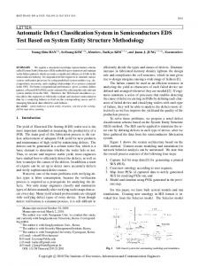
Figure 2. The sample images of nonwoven after image processing: (a) Non defective, (b) tick spot, (c) thin spot, (d) neps After converting the images into black and white the box counting fractal dimension of each image is defined. The graph of figure 3 shows the results of applying the fractal algorithm on one of the defective images. 8
7
6
DB = 1.6812
ln ( N )
5
4
3
2
1 -4.5
-4
-3.5
-3
-2.5 ln ( 1/s )
-2
-1.5
-1
-0.5
Figure 3. The box counting dimension of image (b) Indeed of fractal dimension, density of images is also determined. It is defined as the percent of white pixels to black ones. In table II the results value of the sample that is shown in figure 1 is illustrated. Sample a b c d
Table II: The sample results of applying image processing and fractal dimension mean (pixel) variance std density (%) fractal dimension 81.04 48.28 6.95 0 non 89.45 92.92 9.64 25.18 1.6812 67.16 75.51 8.69 42.11 1.8266 84.65 60.84 7.79 0.23 0.4101
3.3
Neural network algorithm and classification
After feature extraction and determination of each image properties, ie, fractal dimension, density and mean of gray scale image, the two layer neural network is designed and these three parameters of each image is feed as an input. The number of layer and neurons are determined by trail and error. The structure of network is shown in figure 4. The target output must be associated with every input pattern. The numbers of neurons in output layer depend on the number of categories that must be classified. The binary value for output layer is defined. Four classes are considered: 1. non defective (a => code: 1000) 2. thick spot (b => code: 0100) 3. thin spot (c => code: 0010) 4. neps (d => code: 0001) ®
®
V
W
P1
T1 T2
P2
T3 P3
T4
1 Figure 4. The structure of neural network Performance is 4.83927e-005, Goal is 0.0001
0
10
-1
Training-Blue Goal-Black
10
-2
10
-3
10
-4
10
-5
10
0
5
10
15
20 36 Epochs
25
30
Figure 5. The MSE results of training one sample image.
35
4
Conclusion
Defective area of nonwoven is detected and classified using image analysis and neural network algorithms. This algorithm has good advantages comparing other works that were done in this case. One of the best advantages is using fractal dimension. The fractal dimension is not sensitive to the image rotation and also can present the non linearity properties in the source images. By using fractal dimension and density and also the mean value of the gray level of the image, we can reduce the information of each images into only three parameters so the neural network for classification of the images is became very small and the information are reduced very much by keeping the necessary information of the main images. So the training is done very fast and with high accuracy.
5
References
Ahmet AL et al (2000). An Efficient Method For Texture Defect Detection: Subband Domain Co-Occurrence Matrices, Image and Vision Computing, 543-553. Bourke P (1983). Fractal Dimension Calculator User Manual, from World Wide Web http://astronomy.swin.edu.ac. Brzakovic D et al (1996). Designing a defect classification systems: a case study, Pattern Recognition, 29(8), 1401-1419. Campbell JG et al (1997). Flaw detection in woven textile using model based clustering, Irish Machine Vision and Image Processing Conference, University of Ulster. Dar IM et al (1997). Automated pilling detection and fuzzy classification of textile fabrics, Proc. SPIE, Vol. 3029, 26-36. Escofet J et al (1996). Detection of local defects in textile webs using Gabor filters, Proc. SPIE, Vol. 2785, 163- 170 . Frame M et al (2002). Fractal, Graphics & Mathematics Education, The Mathematical Association of America. Huart J et al (1994). Integration of computer vision on to weavers for quality control in the textile industry, SPIE Vol. 2183, 155-164. Karras D et al (1998). Supervised and unsupervised neural network methods applied to textile quality control based on improved wavelet feature extraction techniques, International Journal on Computer Mathematics, Vol. 67, 169-181. Mandelbrot BB ,The Fractal Geometry of Nature, W.H. Freeman and Company (1983). New York. Mueller S et al (1994). Morphological image processing for the recognition of surface defects, Proc. SPIE, Vol. 2249, 298-307. Neural Ware ,Neural Computing: A Technology Handbook for Professional II/PLUS and Neural Works Explorer, Technical Publications Group (1995). Pittsburgh, PA 15275. Norton-Wayne L, Bradshaw M & et al (1992). Machine vision inspection of web textile fabric, Proc. British Machine Vision Conference, 217-226. Olsson LJ et al (1993). Web process inspection using neural classification of scattering light, IEEE Transaction on industrial electronics, Vol. 40, No. 2, 228-234. On line fabric inspection system uses neural networks, fuzzy logic and wavelets to help improve textile quality, (1997). Research News, Georgia Institute of Technology. Pakkanen J et al (2004). The evolving tree- A novel self organizing network for data analysis, Neural Processing Letters, vol. 20, No. 3, 199-211. Peitgen HO et al (1986). The Beauty of Fractals, Images of Complex Dynamical System, Springer-Verlag. Serdaroglu A et al (2004). Defect detection in textile fabric image using wavelet transforms and independent component analysis, Pattern Recognition and Image Understanding, 18-23.
Sezer O G et al (2003). Independent component analysis for texture defect detection, the 6th German-Russian workshop of Pattern Recognition and Image Understanding, Katun Village, Novosibirsk, 210-213. Stojanovic R et al (1999). Automated Detection And Neural Classification Of Local Defects in textile web, Seventh International Conference on image processing-IPA99, Manchester, UK.