Acta Scientiarum http://www.uem.br/acta ISSN printed: 1806-2563 ISSN on-line: 1807-8664 Doi: 10.4025/actascitechnol.v34i4.13020
Application and comparison of level control strategies in the slug flow problem using a mathematical model of the process Airam Sausen*, Paulo Sérgio Sausen, Manuel Reimbold and Maurício de Campos Programa de Pós-graduação Stricto Sensu em Modelagem Matemática, Departamento de Ciências Exatas e Engenharias, Universidade Regional do Noroeste do Estado do Rio Grande do Sul, Rua Lulu Ilgenfritz, 480, 98700-000, Ijuí, Rio Grande do Sul, Brazil. *Author for correspondence. E-mail:
[email protected]
ABSTRACT. This paper presents the application of the error-squared level control strategy Proportional Integral (PI) in the slug flow problem in oil production industry. For this purpose the dynamic model has been used for a pipeline-separator under slug flow with five Ordinary Differential Equations (ODEs), coupled, non-linear. The application of the error-squared level control strategy PI is performed through the methodology by bands, whose objective is to damp the oscillatory flow rate of the load that occur in production separators for equipment downstream of the process. This strategy is compared with the level control strategy PI conventional, widely used in industrial processes; and with the level control strategy PI, also, in the methodology by bands. Simulation results showed that the error-squared level control strategy PI in the methodology by bands, presented better results when compared with the level control strategy PI conventional, because reduced flow fluctuations caused by slug flow; and with the level control strategy PI in the methodology by bands, it probably happened because the first has highly respected the defined bands. Keywords: error-squared controller, band control, slug flow, mathematical modeling.
Aplicação e comparação de estratégias de controle de nível no problema da golfada usando um modelo matemático do processo RESUMO. Neste artigo é apresentada a aplicação da estratégia de controle de nível Proporcional Integral (PI) de erro-quadrático no problema da golfada na produção de petróleo. Para este objetivo é utilizado o modelo dinâmico para uma tubulação-separador em regime de fluxo com golfadas formado por um sistema de cinco Equações Diferenciais Ordinárias (EDO’s), acopladas, não-lineares. A aplicação da estratégia de controle de nível PI de erro-quadrático é realizada considerando a metodologia de controle por bandas, cujo objetivo é amortecer as vazões de carga oscilatórias provenientes das golfadas, que ocorrem em separadores de produção, para os equipamentos a jusante do processo. Esta estratégia é comparada com a estratégia de controle de nível PI convencional, amplamente utilizada em processos industriais; e com a estratégia de controle PI também na metodologia por bandas. A partir da análise dos resultados das simulações, verificou-se que a estratégia de controle de nível PI de erro-quadrático por bandas apresentou os melhores resultados, quando comparada com a estratégia de controle de nível PI convencional, pois reduziu as oscilações de vazão ocasionadas pelas golfadas; bem como com a estratégia de controle de nível PI por bandas, pois respeitou fortemente as bandas definidas. Palavras-chave: controlador de erro-quadrático, controle por bandas, golfadas, modelagem matemática.
Introduction The slug is a multiphase flow pattern that occurs in pipelines which connect the wells in seabed to production platforms in the surface in oil industry. It is characterized by irregular flows and surges from the accumulation of gas and liquid in any cross-section of a pipeline. In this work will be addressed the riser slugging, that combined or initiated by terrain slugging is the most serious case of instability in oil/waterdominated systems (GODHAVN et al., 2005; Acta Scientiarum. Technology
STORKAAS; SKOGESTAD, 2007; SIVERTSEN et al., 2010). The cyclic behavior of the riser slugging, which is illustrated in Figure 1, can be divided into four phases: (i) formation: gravity causes the liquid to accumulate in the low point in pipeline-riser system and the gas and liquid velocity is low enough to enable for this accumulation; (ii) production: the liquid blocks the gas flow and a continuous liquid slug is produced in the riser, as long as the hydrostatic head of the liquid in the riser increases Maringá, v. 34, n. 4, p. 441-449, Oct.-Dec., 2012
442
faster than the pressure drop over the pipeline-riser system, the slug will continue to grow; (iii) blowout: when the pressure drop over the riser overcomes the hydrostatic head of the liquid in the riser the slug will be pushed out of the system; (iv) liquid fall back: after the majority of the liquid and the gas has left the riser the velocity of the gas is no longer high enough to drag the liquid upwards, the liquid will start flowing back down the riser and the accumulation of liquid starts over again.
Figure 1. Illustration of the riser slugging.
The slug flow causes undesired consequences in the whole oil production such as: periods without liquid or gas production into the separator followed by very high liquid and gas rates when the liquid slug is being produced, emergency shutdown of the platform due to the high level of liquid in the separators, floods, corrosion and damages to the equipments of the process, high costs with maintenance. One or all these problems cause significant losses in oil industry. The main one has been of economic order, due to reduction in oil production capacity (GODHAVN et al., 2005). Currently, control strategies are considered as a promising solution to handle the slug flow (FRIEDMAN, 1994; GODHAVN et al., 2005; HAVRE et al., 2000; SKOGESTAD, 2003). An alternative to the implementation of control
Sausen et al.
strategies is to make use of a mathematical model that represents the dynamic of slug flow in pipelineseparator system. In this paper has been used the dynamic model for a pipeline-separator system under the slug flow, conform illustration in Figure 2, with 5 (five) Ordinary Differential Equations (ODEs) coupled, nonlinear, 6 (six) tuning parameters and more than 40 (forty) internal, geometric and transport equations (SAUSEN; BARROS, 2008) that from this moment will be denominated Sausen’s model. To carry out the simulation and implementation of control strategies in the Sausen’s model, first it is necessary to calculate its tuning parameters. For this procedure, are used data from a case study performed by Storkaas and Skogestad (2007) in the OLGA commercial multiphase simulator widely used in the oil industry. Next it is important to check how the main variables of the model change their behavior considering a change in the model's tuning parameters. This testing, called sensitivity analysis, is an important tool to the building of the mathematical models, moreover, it provides a better understanding of the dynamic behavior of the system, for later implementation of control strategies (SAUSEN; SAUSEN, 2010). In this context, from the sensitivity analysis, the Sausen’s model has been an appropriate environment for application of the different feedback control strategies in the problem of the slug in oil industries through simulations. The model enables such strategies can be applied in consequence the slug that is, in the oil or gas output valve separator, as well as in their causes, in the top riser valve, or yet in the integrated system in other words, in more than one valve simultaneously.
Figure 2. Illustration of the pipeline-separator system with the slug formation. Acta Scientiarum. Technology
Maringá, v. 34, n. 4, p. 441-449, Oct.-Dec., 2012
Level control strategies in slug flow problem
443
Therefore, as part of control strategies that can be used to avoid or minimize the slug flow, this paper presents the application of the error-squared level control strategy Proportional Integral (PI) in the methodology by bands, whose purpose damping of the load flow rate oscillatory that occur in production’s separators. This strategy is compared with the level controls strategy PI conventional, widely used in industrial processes; and with the level control strategy PI also in the methodology by bands. Material and methods
separator through the valve Va1, kg s-1; mGS,out(t) is the gas mass flow rate that leaves the separator through the valve Va2, kg s-1; rs is the separator ray, m; H4 is the separator length, m; ρL is the liquid density, kg m-3; VS is the separator volume, m3; VLS is the liquid volume in the separator, m3; Φ
(t ) = m M L L, in − m L, out ( t )
(1)
( t ) =m M G1 G ,in −m G ,1 ( t )
(2)
M G 2 ( t ) = m G int ( t ) − m G , out ( t )
(3)
(t) = N
P G1 ( t ) =
rs2 − (rs − N(t ))2
2H 4 ρ L N( t )[3rs − 2 N( t )]
[m L,out (t) − m LS,out (t)]
[
]
[
ρ LΦ m G, out ( t ) − m GS, out ( t ) + PG1 ( t ) m L, out ( t ) − m LS, out ( t ) ρ L [VS − VLS ( t )]
(4)
]
where: ML(t) is the liquid mass at low point in the pipeline, kg; MG1(t) is the gas mass in the upstream feed section of pipeline, kg; MG2(t) is the gas mass at the top of the riser, kg; N(t) is the liquid level in the separator, m; PG1(t) is the gas pressure in the separator, N m-2; and the M L ( t ) , M G1 ( t ) , M G 2 ( t ) , ( t ) , P ( t ) , are their respective derivatives in N G1 relation to time; mL,in is the liquid mass flow rate that enters the upstream feed section of the pipeline, kg s-1; mG,in is the gas mass flowrate that enters in the upstream feed section of the pipeline, kg s-1; mL,out(t) is the liquid mass flow rate leaving through the valve at the top of the riser enters the separator, kg s-1; mG,out(t), is the gas mass flow rate leaving through the valve at the top of the riser enters the separator, kg s-1; mG,int(t) is the internal gas mass flow rate, kg s-1; mLS,out(t) is the liquid mass flow rate that leaves the Acta Scientiarum. Technology
m mix, out ( t ) = zK1 ρ T (P2 ( t ) − PG1 ( t ))
is a
(6)
where: z is the valve position (0-100%); K1 is the valve constant and a tuning parameter; ρT(t) is the density upstream valve, kg m-3; P2(t) is the gas pressure at the top of the riser, N m-2; PG1(t) is the gas pressure in the separator, N m-2. It is possible to observe that the coupling between the pipeline and the separator occurs through a pressure relationship, in other words, the gas pressure in the separator PG1(t) is the pressure before the Z valve at the top of the riser, according to equation (6). The liquid mass flow rate that leaves the separator is represented by the Va 1 valve equation given by: m LS, out (t ) = z L K 4 ρ L [PG1 (t ) + gρ L N(t ) − POL 2 ]
(5)
RT MG
constant; R is the ideal gas constant (8314 J Kkmol-1); T is the temperature, K; MG is the gas molecular weight, kg mol-1. A simplified valve equation is used to describe the flow through the Z valve at the top of the riser that is given by:
Sausen’s model
In this section has been presented the Sausen’s model that is composed of 5 (five) ODEs based on the mass conservation equations of the system (SAUSEN; BARROS, 2008). The Equations (1) – (3) represent the dynamics of the pipeline system and the Equations (4) and (5) represent the dynamics of the separator.
=
(7)
where: zL is the liquid valve opening (0-100%); K4 is the valve constant and a tuning parameter; g is the gravity (9.81 m s-2); POL2 is the downstream pressure after the Va1 valve, N m-2. The gas mass flow rate that leaves the separator is represented by the Va2 valve equation given by: m GS, out (t ) = z G K 5 ρ G (t )[PG1 (t ) − PG 2 ]
(8)
where: zG is the gas valve opening (0-100%); K5 is the valve constant and a tuning parameter; ρG(t) is the gas density, kg m-3; PG2 is the downstream pressure after the Va2 valve, N m-2. The boundary condition at the inlet (mL,in and mG,in) have been considered constants and disturbances of the process. Following section presents the most critical part of the model that is the phase distribution and phase velocities of the fluids in the pipeline-riser system. Maringá, v. 34, n. 4, p. 441-449, Oct.-Dec., 2012
444
Sausen et al.
equation is given by:
Displacement of the gas flow
The displacement of gas in the pipeline system occurs through a relationship between the gas mass flow and the variation of the pressure inside the pipeline. From physical insight, the two most important parameters determining the gas flow rate at the low point are the pressure drop over, and the free area given by the relative liquid level ε(t) = [H1-h1(t)]/H1, where H1 is the critical liquid level and h1(t) is the liquid level at the low point. This suggests that the gas transport could be described by a valve equation, where the pressure drop is driving the gas through a valve with opening ε(t). Therefore, the equation represents the displacement of the gas flow in pipeline, when h1(t) < H1, is given by: P ( t ) − P2 ( t ) − gρ Lα L ( t )H v G1 ( t ) = K 2ε ( t ) 1 ρ G1 ( t )
(9)
where: vG1(t) is the gas velocity, m s-1; K2 is the valve constant and a tuning parameter; αL is average liquid fraction in riser; P1(t) is the gas pressure in the upstream feed section of the pipeline, N m-2; ρG1(t) is the gas density in the upstream feed pipeline, kg m-3. If h1(t) > H1 the gas velocity vG1(t) = 0. Entrainment equation
The distribution of liquid occurs through an entrainment equation. It is considered that the gas pushes the liquid riser upward, and then the volume fraction of liquid αLT(t) that is leaving through the Z valve at the top of the riser is modelled. The volume fraction of liquid will lie between two extremes: (1) when the liquid blocks the gas flow (vG1(t)=0), there is no gas flowing through the riser and α LT (t ) = α L T (t ) , in most cases there will be only gas leaving the riser, so α L T (t ) = 0 ,
however, eventually the entering liquid may cause the liquid to fill up the riser and α L T (t ) will exceed zero; (2) when the gas velocity is very high there will be no slip between the phases, so α L T (t ) = α L (t ) where αL(t) is the average liquid fraction in the riser. The transition between these two extremes should be smooth and occurs as follows: when the liquid blocks the low point of the riser, the liquid fraction on top is α L T (t ) = 0 , so the amount of liquid in the riser goes on increases until α L T (t ) > 0 . At this
moment the gas pressure and the gas velocity in the feed upstream section of the pipeline is very high, then the entrainment occurs. This transition depends on a parameter q(t). The entrainment Acta Scientiarum. Technology
α LT ( t ) = α L T ( t ) +
where: q(t ) =
[K ρ
qϕ ( t ) 1 + qϕ ( t )
()
(10)
α L ( t ) − α L T ( t )
]
() depend on the gas velocity in [ρ L − ρG1(t )] 2 3 G1 t v G1 t
the system; K3 and φ are tuning parameters of the model. The details of the modeling of the equation (10), the internal, geometric and transport equations for the pipeline system are found in Storkaas and Skogestad (2007), and Sausen and Barros (2008). Simulation and analysis results of the Sausen’s model
In this section are presented the simulation results of the Sausen’s model for a pipelineseparator system. Initially the tuning parameters K1, K2, K3, φ, K4, K5, are calculated considering both the case study data carried out by Storkaas and Skogestad (2007) through the multiphase commercial simulator OLGA, that accurately represents the pipeline system under slug flow, and the data of production separator dimensioned from a tank of the literature (THOMAS, 1999). The tuning procedure for obtaining these parameters can be found in Sausen and Sausen (2010) and Sausen and Barros (2008). Table 1 presents the values of the tuning parameters of the Sausen’s model. Table 1. Sausen’s model tuning parameters.
φ 2,55
K1 0,005
K2 0,8619
K3 1,2039
K4 0,002
K5 0,0003
To verify if the tuning parameters presented in Table 1 are consistent is necessary to carry out the Sausen’s model sensitivity analysis. The sensitivity analysis of a system is defined through the quantification of the change in the dynamic model's variables, given a change in their tuning parameters (KHALIL, 1996). In Sausen and Sausen (2010) is verified that the Sausen’s model was sensitive to the variation of all tuning parameters, being highly sensitive to changes in the K2 parameters in gas velocity equation and K3 in entrainment equation. It is observed that changes in these parameters (i.e., K2 and K3) cause significant changes in the simulation results when compared with the simulation results of the nominal values (i.e., tuning parameters presented in Table 1). It may be stated that the tuning parameters of the Sausen’s model for a pipelineseparator system are properly tuned to in order to consistently represent the slug flow regime in the Maringá, v. 34, n. 4, p. 441-449, Oct.-Dec., 2012
Level control strategies in slug flow problem
445
pipeline-separator system. In this context, the Sausen's model is an appropriate environment for simulated and application of different control strategies to the problem of the slug flow in oil industries. Following are presented the simulation results considering the Z valve opening z = 50% (i.e., slug flow). Figure 3 shows the varying pressures throughout the pipeline system. Figure 4 presents the dynamics of the liquid mass flow rate (up-(a)) and the dynamics of the gas mass flow rate (down-(a)) that are entering the separator with peak mass flow rate of the 15 kg s-1 for the liquid and 2.5 kg s-1 for the gas, and also the dynamics of the liquid mass flow rate (up-(b)) and the dynamics of the gas mass flow rate (down-(b)) that are leaving the production separator. And Figure 5 shows the dynamics of the liquid level (a) and of the gas pressure (b) in the production separator.
75
P1 [Bar] P2 [Bar]
70
Pressure (Bar)
65 60 55 50 45
0
50
100
150
300
350
(b) 15 mLS,out (kg s-1)
15 mL,out (kg s-1)
250
Figure 3. Varying pressures in pipeline system, z = 50%.
(a)
10 5 0
200
Time (min.)
0
50
100
150
200
250
300
10 5 0
350
0
50
100
150
200
250
300
50
100
150
200
250
300
350
2
mGS,out (kg s-1)
mG,out (kg s-1)
2.5 1.5 1 0.5 0
0
50
100
150
200
250
300
0.5 0.4 0.3 0.2
350
0
Time (min.)
350
Time (min.)
Figure 4. Input liquid (up-(a)) and input gas (down-(a)) mass flow rate in the separator, output liquid (up-(b)) and output gas (down(b)) mass flow rate in the separator, z = 50%.
(a)
(b)
0.8
51.5
51
Pressure (bar)
Level (m)
0.75
0.7
0.65
50.5
50
49.5 0.6 0
50
100
150
Time (min.)
49
0
50
100
150
Time (min.)
Figure 5. Liquid level (a) and gas pressure (b) in the separator, z = 50%. Acta Scientiarum. Technology
Maringá, v. 34, n. 4, p. 441-449, Oct.-Dec., 2012
446
It has been observed in all these simulation results that the varying pressures in pipeline system presented in Figure 3 have induced periodic oscillations characterizing the slug flow in pipelineseparator system. It has also been shown that the slug flow happens in 12 min. intervals in separator system. Control strategies
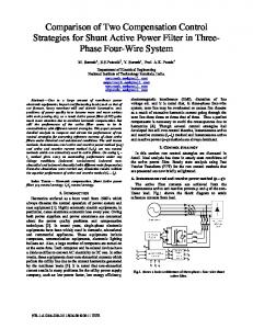
Controller PI actuating in the oil output valve in the oil industry is the traditional method used to control the liquid level in production separators. If the controller is tuned to maintain a constant liquid level, the inflow variations will be transmitted to the separator output, in this case, causing instability in the downstream equipments. An ideal liquid level controller will let the level to vary in a permitted range (i.e., band) in order to make the outlet flow more smooth, this response specification cannot be reached by PI controller conventional for slug flow regime. Nunes (2004) defined a denominated level control methodology by bands, which promotes level oscillations within certain limits, i.e, the level can to vary between the maximum and the minimum of a band, conform Figure 6, so that the output flowrate are close to average value of the input flowrate. This strategy does not use flow measurements, can be applied to any production separator.
Figure 6. Illustration of the band control applied in a two-phase separator.
In the band control when the level is within the band, it is used the moving average of the control action of a slow PI controller, because reducing the capacity of performance of the controller gives a greater fluctuation in the liquid level within the separator. The moving average is calculated in a time interval, this interval should be greater than the period T of the slug flow. When the band limits are exceeded, the control action in moving average of the slow PI controller is switched to the PI controller of the fast action for a time, whose objective is return to the liquid level for within the band, if so, the action of the control again will be the moving average. To avoid abrupt changes in action control for switching between modes of operation Acta Scientiarum. Technology
Sausen et al.
within the band and outside the band, it is suggested to use the average between the actions of PI controller of the fast action and in moving average. Therefore, this paper performs the application in the Sausen's model of the level control strategy PI considering 3 (three) methodologies: (1) level control strategy PI conventional, the level shall remain fixed at setpoint; (2) level control strategy PI in the methodology by bands; (3) error-squared level control strategy PI in the methodology by bands. The error-squared controller (SHINSKEY, 1988) is a continuous nonlinear function whose gain increases with the error. Its gain is computed as: k c (t ) = k1 + k 2 NL e(t )
where: k1 is the linear part, k2NL is the nonlinear one, and e(t ) is the tracking error. When k2NL = 0, the controller is linear, but with k2NL > 0, the controller follows squared-law of the error. In literature the error-squared controller is suggested to be used in liquid level control in production separators under load inflow variations. From the application of the error-squared controller, in liquid level control process in vessels, is observed that small deviations from the setpoint resulted in very little change to the valve leaving the output flow almost unchanged. On the other hand large deviations are opposed by much stronger control action due to the larger error and the law of the errorsquared, thereby preventing the level from rising too high in the vessel. The error-squared controller has the benefit of resulting in more steady downstream flow rate under normal operation with improved response that the level control strategy conventional (SHINSKEY, 1988). For implementations of the controllers is used the algorithm control PI in speed form (CAMPOS; TEIXEIRA, 2006), whose equation is given by: Δu (t ) = k c Δe(t ) + k c
1 Ta e(t ) Ti
where:
Δu (t )
is the variation of the control action; kc is the gain controller; e(t) is the error tracking; Ta is the sampling period of the controller. It is considered that the valve dynamics, i.e., the time for its opening reach the value of the control action is short, so this implies that the valve opening is the control action itself. Maringá, v. 34, n. 4, p. 441-449, Oct.-Dec., 2012
Level control strategies in slug flow problem
447
Results and discussion
the band) uses kc =0.001, k2NL = 0.000004 and Ti = 100000 s, and the PI controller with fast acting (i.e., out the band) uses kc = 0.15, k2NL = 0.03 and Ti = 1000 s. The period for calculating the moving average of the PI controllers by band was T = 1000 s. Figure 7a presents the liquid level variations N(t) considering level controller strategy PI conventional (dashed line) and level control strategy PI in the methodology by bands (solid line) in the separator, and the Figure 7b presents liquid level variations N(t) considering level control strategy PI conventional (dashed line) and error-squared level control strategy PI in methodology by bands (solid line). Figures 8a and b shown the liquid output flow rate variations of the separator that corresponding to controls of the presented in Figures 7a and b. The following are presented simulation results for valve opening at the top of the riser, i.e., z = 20%, z = 25%, z = 30% and z = 35% (slug flow). Figure 9a presents the liquid level variations N(t) considering level control strategy PI conventional (dashed line) and level control strategy PI in the methodology by bands (solid line) in separator, and the Figure 9b presents liquid level variations N(t) considering level control strategy PI conventional (dashed line) and errorsquared level control strategy PI in the methodology by bands (solid line). Figures 10a and b shown the liquid output flow rate variations of the separator that corresponding to controls of the level presented in Figure 9a and b.
This section presents the simulation results of the control strategies using the computational tool Matlab. To implement the control by bands is used a separator with length 4.5 m and diameter 1.5 m following the standards used by Nunes (2004). The setpoint for the controller is 0.75 m (i.e., separator half), the band is 0.2 m, where the liquid level maximum permitted is 0.95 m and the minimum is 0.55 m. The bands were defined to follow the works of Nunes (2004). Initially, for the first simulation, it is considered the Z valve opening at the top of the riser in z = 20% (slug flow). To simulate the level control strategy PI conventional the values used for the controller gain kc and the integral time T i are 10 and 1380 s respectively, according to the heuristic method to tune level controllers proposed by Campos and Teixeira (2006). In level control strategy PI in the methodology by bands the level can float freely within the band limits in separator. In this case, the controller PI with slow acting (i.e., within the band) uses controller gain kc = 0.001 and integral time Ti = 100000 s, and the PI controller with fast acting (i.e., out the band) uses kc = 0.15 and Ti = 1000 s. In errorsquared control strategy PI in the methodology by bands, the gain linear and nonlinear of the controller are computed to following the methodology based on Lyapunov stability theory (KHALIL, 1996). In this case, the error-squared level PI controller with slow acting (i.e., within (a) 1.2
Setpoint. PI conventional level controller. PI level controller by bands.
1.1
1
1
0.9
0.9
0.8
0.8
0.7
0.7
0.6
0.6
0.5
Setpoint. PI conventional level controller. Error-squared PI level controller by bands.
1.1
Level (m)
Level (m)
(b) 1.2
0
50
100
150
200
250
Time (min.)
300
350
400
0.5 0
50
100
150
200
250
300
350
400
Time (min.)
Figure 7. Liquid level variations N(t), (a) level control strategy PI conventional (dashed line) and level control strategy PI by band (solid line), (b) level control strategy PI conventional (dashed line) and error-squared level control strategy PI by band (solid line), z = 20%. Acta Scientiarum. Technology
Maringá, v. 34, n. 4, p. 441-449, Oct.-Dec., 2012
448
Sausen et al. (a)
(b)
20
Output flowrate variations with PI conventional level controller. Output flowrate variations with PI level controller by bands.
16
16
14 12 10 8 6
14 12 10 8 6
4
4
2
2
0
0
50
100
150
200
250
300
350
Output flowrate variations with PI conventional level controller. Output flowrate variations with error-squared PI level controller by bands.
18
Output flowrate (kg s-1)
18
Output flowrate (kg s-1)
20
0
400
0
50
100
150
Time (min.)
200
250
300
350
400
Time (min.)
Figure 8. Liquid output flow rate variations mLS,out(t), (a) level control strategy PI conventional (dashed line) and level control strategy PI by band (solid line), (b) level control strategy PI conventional (dashed line) and error-squared level control strategy PI by band (solid line), z = 20%. (a) 1.2
Setpoint. PI conventional level controller. PI level controller by bands.
1.1 1
1
0.9
0.9
0.8 0.7
0.8 0.7
0.6
0.6
0.5
0.5
0.4
0.4 0
50
100
150
200
250
300
Setpoint. PI conventional level controller. Error-squared PI level controller by bands.
1.1
Level (m)
Level (m)
(b) 1.2
350
400
0
50
100
150
Time (min.)
200
250
300
350
400
Time (min.)
Figure 9. Liquid level variations N(t), (a) level control strategy PI conventional (dashed line) and level control strategy PI by band (solid line), (b) level control strategy PI conventional (dashed line) and error-squared level control strategy PI by band (solid line), z variable. (a)
14 12 10 8 6 4
Output flowrate variations with PI conventional level controller. Output flowrate variations with error-squared PI level controller by bands.
20 18
Output flowrate (kg s-1)
Output flowrate (kg s-1)
(b)
Output flowrate variations with PI conventional level controller. Output flowrate variations with PI level controller by bands.
16
16 14 12 10 8 6 4
2 0
2 0
50
100
150
200
250
Time (min.)
300
350
400
0
0
50
100
150
200
250
300
350
400
Time (min.)
Figure 10. Liquid output flowrate variations mLS,out(t), (a) level control strategy PI conventional (dashed line) and level control strategy PI by band (solid line), (b) level control strategy PI conventional (dashed line) and error-squared level control strategy PI by band (solid line), z variable. Acta Scientiarum. Technology
Maringá, v. 34, n. 4, p. 441-449, Oct.-Dec., 2012
Level control strategies in slug flow problem
Comparing the simulation results between the level control strategy PI and error-squared level control strategy PI both in the methodology by bands, it is observed that the second controller (Figures 7 and 9b) has respected strongly the defined bands, i.e., in 0.95 m (higher band) and in 0.55 m (lower band), because it has the more hard control action than the first controller (Figures 7 and 9a). However, when the liquid level reached the band limits for the error-squared level control strategy PI, at this time, the liquid output flow rate has a little more oscillatory flows than the ones found for the level controller PI by bands, but this difference is minimal, according to Figures 8a and b, Figures 10a and b. For both controllers simulation results of the liquid output flow rate are better than the results obtained with the level control strategy PI conventional. Considering the liquid output flow rate when the level is within the band, both processes (i.e., level control strategy PI and error-squared level control strategy PI both in the methodology by band) have similar trends. Conclusion In this paper three methodologies of the level controls, considering the slug flow problem in oil industry, were implemented: (1) level control strategy PI conventional; (2) level control strategy PI by bands; (3) error-squared level control strategy PI by bands. The simulation results showed that the third methodology presented the better results, because reduced flow fluctuations caused by slug flow when compared to other methods tested. As suggestions for future work new control strategies can be implemented, a model with fewer parameters can be investigated, and an experimental platform can be constructed. References CAMPOS, M. C. M.; TEIXEIRA, H. C. G. Controles típicos de equipamentos e processos industriais. 1. ed. Rio de Janeiro: Editora Edgard Blücher, 2006.
Acta Scientiarum. Technology
449
FRIEDMAN, Y. Z. Tuning of averaging level controller. Journal of Hydrocarbon Processing, v. 73, n. 3, p. 101-104, 1994. GODHAVN, M. J.; MEHRDAD, F. P.; FUCHS, P. New slug control strategies, tuning rules and experimental results. Journal of Process Control, v. 15, n. 5, p. 547-577, 2005. HAVRE, K.; STORNES, K.; STRAY, H. Taming slug flow in pipelines. Journal of Oil and Gas, v. 4, n. 1, p. 55-63, 2000. KHALIL, H. K. Nonlinear systems. 2nd ed. New Jersey: Prentice Hall, 1996. NUNES, G. C. Control for bands to primary processing: application and fundamental concepts. Rio de Janeiro: Cenpes, 2004. (Report of the Petrobras - Cenpes). SAUSEN, A.; BARROS, P. R. Modelo dinâmico simplificado para um sistema encanamento-riser-separador sob regime de fluxo com golfadas. Tendências em Matemática Aplicada e Computacional, v. 9, n. 2, p. 341-350, 2008. SAUSEN, A.; SAUSEN P. S. Aplicação de uma metodologia para a análise da sensibilidade do modelo dinâmico para uma tubulação-separador sob golfadas. Tendências em Matemática Aplicada e Computacional, v. 11, n. 3, p. 245-256, 2010. SHINSKEY, F. G. Process control systems: application, design, and adjustment. 2nd ed. New York: McGraw-Hill Book Company, 1988. SKOGESTAD, S. Probably the best simple PID tuning rules in the world. Journal of Process Control, v. 14, n. 4, p. 291-309, 2003. SIVERTSEN, H.; STORKAAS, E.; SKOGESTAD, S. Small-scale experiments on stabilizing riser slug flow. Journal Chemical Engineering Research and Design, v. 88, n. 2A, p. 213-228, 2010. STORKAAS, E.; SKOGESTAD, S. Controllability analysis of two-phase pipeline-riser systems at riser slugging conditions. Journal of Control Enginnering Practice, v. 15, n. 5, p. 567-581, 2007. THOMAS, F. Simulation of industrial processes for control engineers. Oxford: Butterworth-Heinemann, 1999. Received on March 30, 2011. Accepted on July 18, 2011.
License information: This is an open-access article distributed under the terms of the Creative Commons Attribution License, which permits unrestricted use, distribution, and reproduction in any medium, provided the original work is properly cited.
Maringá, v. 34, n. 4, p. 441-449, Oct.-Dec., 2012