Application Identification Based on Network Behavioral Profiles Yan Hu
Dah-Ming Chiu
John C. S. Lui
Dept. of Information Engineering Chinese University of Hong Kong Email:
[email protected]
Dept. of Information Engineering Chinese University of Hong Kong
[email protected]
Dept. of Computer Science & Engineering Chinese University of Hong Kong Email:
[email protected]
Abstract— Accurate identification of network applications is important to many network activities. Traditional port-based technique has become much less effective since many new applications no longer use well-known fixed port numbers. In this paper, we propose a novel profile-based approach to identify traffic flows belonging to the target application. In contrast to classifying traffic based on statistics of individual flows in previous studies, we build behavioral profiles of the target application, which describe dominant patterns of the application. Based on the behavior profiles, a two-level matching is used in identifying new traffic. We first determine if a host participates in the target application by comparing its behavior with the profiles. Subsequently, for each flow of the host we compare if it matches with those patterns in the application profiles to determine which flows belong to this application. We demonstrate the effectiveness of our method on campus traffic traces. Our results show that one can identify the popular P2P applications with very high accuracy.
I. I NTRODUCTION Accurate identification of network applications is important in many areas such as network planning, quality of service (QoS) and access control. To identify network applications, the simplest method is to use transport layer port numbers, since many services are supposed to run on well-known ports. However, nowadays this traditional port-based technique has become much less accurate for many reasons. For instance, some popular new applications, such as P2P applications, do not rely on predefined well-known ports. Another reason is that firewalls block some unauthorized or unknown applications, so some applications are tunneled through port 80 to circumvent firewalls. Another approach is payload-based analysis, which search packet payloads for signatures of known applications. This approach is employed in some commercial network management products. However, finding appropriate signatures for some applications (in particular, newly released applications), and maintaining an up-to-date signatures for various applications are daunting tasks. Moreover, payload-based method is ineffective when traffic is encrypted. Recently, some novel approaches ([9], [17], [19]) try to classify network traffic relying on statistical observations of the flows. These approaches develop discriminating criteria based on the statistical observations (such as the packet size distribution per flow, flow duration, and the statistics of the inter-arrival times between packets in flows, etc.), and then employ clustering, classification and other machine learning
techniques to classify traffic. These methods provide a promising alternative for traffic classification. There are two challenges in identifying applications using flow properties. First, different flows in the same application may have different flow statistics, especially when patterns of some new applications are increasingly complex. For example, in the P2P file-sharing applications, some flows are used to get peer information, other flows are to negotiate between peers, and other flows are involved in the actual file transfer. These various kinds of flows have different statistics and even different transport protocols (TCP or UDP). Second, the flows in different applications may have similar statistics. There will be false positive if only per-flow statistics is used. In this paper, we propose a new approach to identify network applications, and our approach has two novelties. The first one is profile-based. That is, in addition to observing statistics of individual flows, we build profiles for a given application, which describe communication patterns of this application. The second one is two-level matching. The first level determines if a host participates in a given application by comparing its behavior with the profiles of this application. Since a host may take part in different applications at the same time, we then compare each flow of the host with the profiles to determine which flow belongs to this application and which one does not. The two properties of our approach can improve the accuracy of identifying network applications. As we have mentioned, new applications are increasingly complex and different kinds of flows within an application may have different properties. Profiles are the set of most significant properties of this application. Comparing a host’s behavior with the profiles is equivalent to look at properties of multiple flows of this host, which contain more information than a single flow. Moreover, although flows in different applications may have similar statistics, in our two-level matching, we first locate those hosts that participate in the application and then classify their flows, which can reduce false positive. To build behavioral profiles for network applications, the first step is to choose appropriate features that are used in profiles. After that, we observe properties of flows that are contained in the target application. Since manually extracting properties from large numbers of flows is difficult and time consuming, we use a data mining technique named association
mining in this step. Having obtained the association rules, we look back at the behavior of those hosts that participate in the application and construct profiles. Finally, in the application identification step, matching is implemented in two levels, host level and flow level. The rest of the paper is organized as follows. We describe related work in Section II. Before describing our approach in detail, we first give an example of application profiles in Section III. After that, we discuss the flow features that are chosen to construct application profiles in Section IV, and explain how to build behavioral profiles for the target application in Section V. In Section VI, we describe the two-level matching method to identify the application in new traffic. Experimental results are given in Section VII. Finally, we conclude our paper in Section VIII. II. R ELATED W ORK Due to its fundamental nature, the field of traffic classification has received continuous interest. Some traffic classification approaches develop discriminating criteria based on statistical observations of various flow properties in the packet traces. Based on these statistical observations, these studies employ classification, clustering and other machine learning techniques to assign flows to classes. Roughan et al. in [19] classify traffic flows into four classes suitable for quality of service applications. They demonstrate the performance of Nearest Neighbor and Linear Discriminant Analysis algorithms. Moore et al. in [17] apply Bayesian analysis techniques to categorize traffic by application. In addition to these trained classification techniques, unsupervised clustering methods are also used in several studies. The work of Campos et al. in [11] applies a number of different hierarchical clustering methods presented as dendrograms to identify groups of similar communication patterns. Similarly, in [16], McGregor et al. seek to identify traffic with similar observable properties and apply a probabilistic clustering method (the EM algorithm) to this problem. In [8], Erman et al. evaluate and compare several clustering algorithms in traffic classification, including K-Means, DBSCAN and AutoClass algorithms. In [6], Bernaille et al. evaluate the feasibility of application identification at the beginning of a TCP connection. This approach distinguishes the behavior of an application by observing the size and the direction of the first few packets of the TCP connection. Most of these studies which apply machine learning techniques only focus on statistics of a single flow, while our approach observes patterns of multiple flows. Another promising traffic classification approach is shown in [13], which is closer to our work. Instead of classifying individual flows, Karagiannis et al. propose to associate Internet hosts with applications, and then classify their flows accordingly. They attempt to capture the inherent behavior of a host at three levels of increasing detail: the social, the functional and the application level. This approach mainly focuses on higher level communication patterns such as the
number of source ports a particular host uses for communication, and does not make use of flow statistics that we utilize. Concurrent to [13], Xu et al. in [22] use information theoretic and data mining techniques to build behavior profiles of Internet backbone traffic. The stunning growth of P2P traffic has drawn more attention from researchers recently. Several studies emphasize on identification of P2P traffic, such as the signature-based payload methodology in [20] and the identification method by transport layer characteristics in [12]. In [7], Collins et al. propose a set of tests for identifying masqueraded peer-to-peer file-sharing applications. III.
AN
E XAMPLE OF A PPLICATION P ROFILE
Before describing our approach in detail, we first give an example of application profiles in this section. We take a popular peer-to-peer file-sharing application, BitTorrent, as an example. The BitTorrent network consists of clients and a centralized server. Clients (named downloaders) connect to each other directly to send and receive pieces of a file. The central server (named tracker) coordinates the action of the downloaders. Instead of describing protocol details, here we focus on flow properties of communication between downloaders and between the downloader and the tracker. We also describe corresponding payload signatures in different traffic, which are used in training and validation. However, payload signatures are not contained in application profiles. There are roughly four kinds of traffic in a BitTorrent application: 1) users download the .torrent files, 2) downloaders periodically check in with the tracker, 3) peers communicate with each other, and 4) communication between DHT nodes. To download a file, a user should first get the corresponding .torrent file. This step is usually done over HTTP and completed in one connection, so this kind of traffic is negligible. Downloaders periodically check in with the tracker to keep it informed of their progress and receive lists of peers, which operates over TCP. Many of these flows have the signature of “get /anounce?” in the payload. We call the direction from the connection initiator to the acceptor request direction, and the reverse direction response direction. For some of the flows, in addition to the three-way handshake in TCP connection establishment and the four-way handshake in connection termination, there is one packet in the request direction and one packet in the response direction, and the sizes of the request packets in different flows are similar. Properties of these flows can be summarized as the following rule: rule1: TCP, the same source IP, 5 request packets, 4 response packets, fixed size in request bytes Rule1 means that there are some TCP connections, which are sent from the same source IP address. Each connection has 5 request packets and 4 response packets, and the total number of bytes in these request packets are fixed. Other flows may have different properties. For example, the packet number in TCP connection termination is less than 4, so the numbers of request packets or response packets are different from the
ones in rule1. Properties of these flows can be represented by another rule. The third kind of traffic is between downloaders. Downloaders upload and download files from each other via direct connections. In the original protocol, this traffic operates over TCP. Later in some extended versions, UDP is also used. Most of these flows have the payload signature “bittorrent protocol”. An example of flow properties of this kind of traffic is in rule2. Rule2 represents properties of those flows that are used to download files, so they have large flow duration, large number of response packets and response bytes. rule2: TCP, the same source IP, the number of response packets > 400, the number of response bytes > 100000, flow duration > 20 second The fourth kind of traffic is communication between DHT nodes. In trackerless DHT protocol ([1]), BitTorrent uses a “distributed sloppy hash table” (DHT) for storing peer contact information for “trackerless” torrents. In effect, each peer becomes a tracker. BitTorrent clients include a DHT node, which is used to contact other nodes in the DHT to get the location of peers to download from. This protocol is implemented over UDP. Payload signature “d1:ad2:id20:” and “d1:rd2:id20:” present in this kind of traffic. Several examples of flow properties are as follows: rule3: UDP, the same source IP, the same source port, 1 request packet, 1 response packet, fixed size in request bytes, fixed size in response bytes rule4: UDP, the same source IP, the same source port, 1 request packet, 0 response packet, fixed size in request bytes rule5: UDP, the same source IP, the same source port, 2 request packets, 2 response packets, fixed size in request bytes Rule3 is one example for the “GET PEERS” request in DHT protocol. All flows are from the same source IP address and the same source port number. There are one request packet and one response packet, and both have the fixed number of bytes in all flows. Rule4 is the case that there is no response for the “GET PEERS” request, so the number of response packet is 0. Rule5 is an example for an “ANNOUNCE PEER” message after the “GET PEERS” request, so there are two request packets and two response packets. From the above example, we can find that the complex applications (such as P2P applications) have several types of traffic which is different from each other. There are even different cases in each type of traffic. We summarize the properties of the flows in each type of traffic in rules like rule1 - rule5. Flow properties include the transport layer information (such as protocol, whether all flows use the same IP address and/or the same port number) and statistical information (such as the number of packets, the number of bytes and flow duration etc.). Profiles of an application are a set of such rules, which characterize the most important communication patterns of this application. IV. F LOW F EATURES C OLLECTION To build profiles, the first question is to determine what features should be chosen to construct profiles and how to collect
statistics duration rpack(ppack) rbyte(pbyte) rsizeavg(psizeavg) rsizevar(psizevar) rduravg(pduravg) rdurvar(pdurvar) rhbyte1(phbyte1) rhbyte2(phbyte2)
meaning the flow duration the number of packets in request (response) direction the number of bytes in request (response) direction the average packet size in request (response) direction variance of the packet size in request (response) direction the average inter-arrival time between packets in request (response) direction variance of inter-arrival time between packets in request (response) direction the size of the first data packet in request (response) direction the size of the second data packet in request (response) direction TABLE I T HE FLOW STATISTICS .
these features. As we have mentioned, application profiles are a set of rules and each rule summarizes the common properties shared by a number of flows in the application, which include transport layer properties and statistical properties. We focus on properties of bidirectional flows, also known as connections. The reason is that we need to differentiate statistical observations of the request and the response direction, which are different in many applications. Typically, a flow is defined by the five tuples: {srcIP, destIP, srcPort, destPort, protocol}. We use the five tuples to study transport layer properties. In addition, flow statistics are also chosen as flow features to study statistical properties. Previous studies ([17], [21], [23]) investigate the issue of feature selection and dimension reduction in traffic classification. Based on the previous studies and our own experiences, we choose several flow statistics, as summarized in Table I. With the exception of flow duration, the other flow statistics are calculated in the request and response direction separately. For the number of bytes (or packet size), we only calculate the payload size, since the sizes of IP and TCP/UDP headers are not important for application identification. Besides the flow statistics that are commonly used, we add four additional statistics to represent the size of the first (second) data packet in the request (response) direction, as shown in the last two rows of Table I. The first data packet means the first packet after the three-way handshake in TCP connection establishment. For UDP protocol, its first packet is also the first data packet. The first few packets in connections are important for application identification since they usually capture the application’s negotiation stage. The flow features that are chosen to construct application profiles are the five tuples plus all the flow statistics summarized in Table I. To collect the flow features, we process packet traces with Bro ([18]), an open-source network intrusion detection system. All the flow statistics can be updated online in a streaming fashion, which means that we do not need to store data per packet, but rather per connection. For a series
of data Xj , its average and variance can be easily calculated in a streaming fashion using the following equations: j 1 Xj+1 + Xj j+1 j+1 j−1 1 var(Xj+1 ) = var(Xj ) + (Xj+1 − X j )2 j j+1 X j+1 =
(1) (2)
where X j and var(Xj ) are the average and variance of the first j samples of data. Xj can represent the packet size and the inter-arrival time between packets of a flow. V. A PPLICATION P ROFILES In this section, we explain how to build profiles for a given application. To build application profiles, training traces are needed. In the training traces, we know in advance which traffic belongs to this application and which does not. Having the training trace, we extract common properties shared by some flows of the application. Finally, we build application profiles based on the resulted flow properties. A. Training Traces We first provide a quick description of the datasets used in our study. The datasets are packet traces collected in the gateway of our department. We captured the packet header and the first 42 bytes of payload of the traffic through the gateway. For privacy considerations, we anonymize all the IP addresses using “anontool” ([2]). Based on the requirement of the network administrator, we also strip the payloads of some well-known applications which may reveal the url, email address, and other information. These packet traces are used for training and validation. We first use Bro to process the packet traces to get connection records. Each connection record contains the flow features that are used to construct profiles. To serve as training traces, the connections that belong to the target application should be labelled. For application identification, we only need to label those connections that participate in the application, and do not need to determine the applications of other connections. However, in traffic classification, all connections should be labelled as one target class, which is more difficult. Determining the true “applications” of the connections is a difficult task. We combine several methods to identify the target application, including payload-based method, {IP, port} pairs, and even manual analysis. In payload-based method, protocol signatures are identified either from previous studies ([13], [20]) and public documents, or by reverse-engineering. We add functions to Bro such that it matches the signatures of a given application in packet payloads and labels the corresponding connection records. For example, the signature of BitTorrent is represented by this regular expression: “∧ get /announce\? | bittorrent protocol | d1:ad2:id20: | d1:rd2:id20: | ∧ azver”. Not all flows in the target application have traceable signatures. We use {IP, port} pairs and even manual analysis to assist identification. {IP, port} pairs associate a particular IP address and a specific port with one application, since the
service reflected at a specific port for a specific IP does not change within a short period. For example, if connection C1 and C2 have the same source IP and the same source port and within the same time interval, then we consider that C1 and C2 are involved in the same application. Note that this method may have problem in some case of Network Address Translation (NAT), which does not appear in our datasets. B. Extract Flow Patterns As we have mentioned, network applications have different types of traffic, and flows in each type of traffic share some common properties. We call these common properties flow patterns, as summarized in rule1 - rule5. Profiles of an application are a set of such rules. Manually extracting flow patterns from large numbers of flows is hard and time-consuming. We use data mining techniques for the extraction of frequent itemsets and association rules ([10]) in this step. Association rule mining is to find inter-relationships (correlations) between members of a data set. The application of association rule mining to network traffic is widely deployed in the realm of network security, especially intrusion detection ([14], [15]), and recently in traffic analysis ([5]). A set of items is referred to as an itemset. The occurrence frequency of an itemset is the number of transactions that contain the itemset, which is also known as the support of the itemset. If the support of an itemset I satisfies a predefined minimum support threshold, then I is a frequent itemset. Association rules are extracted from frequent itemsets and show correlations among contained elements. Association rules are usually in this form: A ⇒ B (support, conf idence), where A and B are itemsets, and A ∩ B = φ. A is often referred to as the body of the rule, while B as the head of the rule. The support is the number of transactions that contain A ∪ B, divided by the total number of transactions. The confidence is the support of sets that contain A ∪ B, divided by the support of sets that contain A. Finally, we have: support(A ⇒ B) = P (A ∪ B) support(A ∪ B) conf idence(A ⇒ B) = P (B|A) = support(A)
(3) (4)
In general, association rule mining can be viewed as a twostep process: 1) find all frequent itemsets that occur at least as frequently as a predetermined minimum support count, 2) generate association rules from the frequent itemsets, which must satisfy minimum support and minimum confidence. Apriori ([4]) is a widely used algorithm for mining frequent itemsets and association rules. Association rule mining satisfies our needs of extracting common properties shared by some flows (flow patterns) from a large number of flows, since we need to discover correlations between flow patterns and the target application. Based on the flow features and the application label, we develop various attributes for the flows. Each flow is represented in the form of {attribute1 = value1 , ..., attributen = valuen }. The attributes are those flow features and the application label. The values are corresponding value of each attribute.
The problem is that Apriori is an algorithm for mining frequent itemsets for Boolean association rules. However, the flows have richer attribute types. The five tuples of flows are categorical, while other flow statistics are quantitative. Boolean attributes can be considered as a special case of categorical attributes. Categorical attributes can be processed by Apriori using the following method. We input transactions in the form of {srcPort = 2119, destPort = 80, ...} to Apriori, then Apriori will regard “srcPort = 2119” as a boolean attribute, instead of regarding “srcPort” as a categorical attribute. Different from categorical attributes, quantitative attributes can not be simply processed as boolean attributes. Quantitative attributes have different types (some are in integer, e.g., rpack and rbyte, and others are in float, e.g., duration, rsizeavg, and rsizevar), and a wide range of values defining their domain. In addition, quantitative attributes have an implicit ordering among values. For example, {rbyte = 150} and {rbyte = 151} are similar statistical observations for the attribute “rbyte”. To do this, we first partition the ranges of those quantitative attributes into “bins”. The partitioning strategy that we use is equal-frequency binning ([10]), where each bin has approximately the same number of tuples assigned to it. Another common strategy is equal-width binning where the interval size of each bin is the same. We choose equalfrequency binning rather than equal-width binning because of the uneven distribution of these quantitative attributes. With the partitions of the quantitative attributes, we then replace the exact values of the flow attributes with the ranges of the bins that the exact values are in. An example is given below: Example 1: {srcIP = 193.169.140.183, srcPort = 3946/6, rpack = 11, rbyte = 408...450, duration = 4.0...22870.5, rsizeavg = 34.7...43.1, rhbyte1 = 156, rhbyte2 = 168, ... , signame = bittorrent}. We regard the five tuples of a flow as four keys: (srcIP, destIP, srcPort, destPort), because port numbers are meaningful only when combined with protocol type. In the example, “srcPort = 3946/6” means the port number is 3946 and the protocol type is 6 (TCP). Some bins only have one value because there are enough flows having this value for the corresponding attribute (e.g., rpack). As for the four flow features rhbyte1, rhbyte2, phbyte1, and phbyte2, they are intended to capture the application’s negotiation stage. Therefore, their actual values are kept, and no partition is processed. “signame = bittorrent” means this connection is identified as “BitTorrent”. The only parameter that need to be set in this step is the number of bins for each quantitative attributes. We choose a larger number of bins for the packet number and byte number (eg. 30 for rpack and rbyte), and a smaller number of bins for duration and inter-arrival time between packets(eg. 5 for duration). For flow duration, we only care about the flow is short or long, and the inter-arrival time between packets would be affected by network conditions. To automatically extract common properties shared by partial flows of the target application from the large number of flows, we input all flows in the trace file in the form as in Example 1 to Apriori ([3]). To improve efficiency and reduce
the number of association rules that are generated, we restrict the head of the rules to the target application, since we want to discover the correlations between flow patterns and the target application. Examples of the resulted association rules are given below: Example 2: signame = bittorrent ⇐ srcIP = 193.169.140.183, srcPort = 19270/17, rpack = 1, ppack = 1, rbyte = 98, pbyte = 272, duration = 0.6 ... 2.9 (0.40/721, 100.0) signame = bittorrent ⇐ srcIP = 193.169.140.183, srcPort = 19270/17, rpack = 1, ppack = 0, rbyte = 98 (0.80/1311, 100.0) Example 2 illustrates the association rules that are generated by Apriori. The head of all the rules are restricted to “signame = bittorrent” when the target application is “BitTorrent”, and the body of the rules contains various flow properties. For “(0.40/721, 100.0)”, 0.40 means the support of this rule is 0.4%, 721 means there are totally 721 connections having the properties that are shown in the body of the rule, and 100.0 means the confidence of the rule is 100%. We need to provide min sup and min conf when using Apriori for association mining. Tuning these two parameters is a big challenge for association mining. A meaningful setting may become ineffective when used in another trace file. However, our method only applies association mining to get all potential flow patterns, which are selected again in later steps of building application profiles. Therefore, in this step, we choose low values for min sup and min conf to guarantee low false negative. The false positive can be reduced in later steps. We set min conf = 80%. min sup is set based on the number of connections belonging to the target application (app num) instead of the total number of connections in the training trace file (conn num), since conn num is similar for each trace file while app num varies much. min sup is set to be 2.5% of app num. C. Build Application Profiles Having these flow patterns, the next step is to build profiles for the target application. There are several issues that need to be considered. Firstly, there are usually a large number of association rules generated from Apriori, how can we reduce the number of rules by removing redundant rules and keeping meaningful ones. The second issue is how to get a complete set of flow patterns. As we know, network applications may have different versions of software implementation. In addition, different configuration or even different user may result in various flow patterns. Therefore, we need to combine different flow patterns together to get a complete set. The third question is that, among the whole set of flow patterns, which ones constitute a profile? In other words, when the target application occurs, which flow patterns usually appear together. In the remaining part of this section, we first present our algorithm for building application profiles in Section V-C.1, and then discuss how to settle the first two problems in Section V-C.2, and how to settle the third problem in Section V-C.3. 1) Algorithm Description: Algorithm 1 describes the main steps of building application profiles, with tapp denotes the
Algorithm 1 Build Application Profiles Initialization: tapp = the target application, gT cprul = ∅, gU dprul = ∅, gP rof ile = ∅; 1. partition quantitative attributes; 2. for the ith training trace file 3. label all connections of tapp; 4. collect features for each connection; /* process for TCP */ 5. tcpAssorule(i) = Apriori (all tcp connection); 6. tcpRule(i) = MaximalAssorule (tcpAssorule(i)); 7. gT cprul = MergeRule (gT cprul, tcpRule(i)); /* process for UDP */ 8. udpAssorule(i) = Apriori (all udp connection); 9. udpRule(i) = MaximalAssorule (udpAssorule(i)); 10. gU dprul = MergeRule (gU dprul, udpRule(i)); 11. endfor 12. gP rof ile = ConstructProfile(gT cprul, gU dprul);
target application. The outputs of Algorithm 1 are three lists: gT cprul contains global rules for TCP protocol, gU dprul contains global rules for UDP protocol, and gP rof ile contains the final application profiles. The three lists are all empty at initialization. We have discussed steps in line 1 - line 4 in previous sections. The first step is to partition the ranges of the quantitative attributes into intervals, as described in Section V-B. After that, we choose several training trace files. For each file, we label all connections that are identified as tapp using the methods explained in Section V-A, and then collect features for each connection as described in Section IV such that each connection is represented in the form as Example 1. After the preparative steps in line 1 - line 4, we input all connections in a training trace file to Apriori for association rule mining. We use all connections instead of only the connections belonging to tapp for mining since we need some background data. If we only use the connections belonging to tapp, we can not make sure the resulted association rules are unique for tapp. In other words, other applications may also have the patterns described by the association rules. We mine TCP and UDP connections separately, as shown in the steps of line 5 and line 8. In the two steps, a minimum support (min sup) and a minimum confidence (min conf ) should be provided to Apriori. The remaining lines of Algorithm 1 will be explained in the next two sections. 2) Process Association Rules: A major challenge in association rule mining from a large data set is the fact that such mining often generates a huge number of frequent itemsets and association rules satisfying min sup and min conf , especially when they are set low. To overcome this difficulty, the concepts of closed frequent itemset and maximal frequent itemset are introduced ([10]). An itemset X is a closed frequent itemset in a data set S if X is frequent, and there exists no proper super-itemset Y such that Y has the same support as X in S. An itemset X is a maximal frequent itemset in S if X is frequent, and there exists no super-itemset Y such
that X ⊂ Y and Y is frequent in S. As shown in Example 2, the head of the association rules are restricted to “signame = tapp”, and the body of the rules contains various flow properties. We want the body to contain more flow properties, so maximal association rules are kept. In other words, we keep the association rule r1 “signame = tapp ⇐ B1” if r1 satisfies min sup and min conf , and there exists no association rule r2 “signame = tapp ⇐ B2” such that B1 ⊂ B2 and r2 satisfies min sup and min conf . Here, B1 and B2 are itemsets with items in the form of “attributei = valuei ”. We do this process in line 6 for TCP and line 9 for UDP, which can greatly reduce the number of association rules while keep most of the information. Network applications usually have different versions of software implementation. In addition, different configuration or even different user may result in different flow patterns. Therefore, we will get different association rules from each training trace files, denoted by tcpRule(i) and udpRule(i). To get a complete set of flow patterns, we merge different rules together to get the global rules gT cprul and gU dprul, as described in line 7 and line 10. Flows are defined by the four keys: (srcIP, destIP, srcPort, destPort). In merging rules, these four keys are treated differently from other flow statistics described in Table I. For IP address and port number, we only care if the flows are sent from (or received by) the same IP address and port number, and do not care about the specific values. Therefore, if there are two rules r1 and r2, r1 : signame = tapp ⇐ a1 = vx1 , ..., aj = vxj , aj+1 = vxj+1 , ..., ak = vxk r2 : signame = tapp ⇐ a1 = vy1 , ..., aj = vyj , aj+1 = vyj+1 , ..., ak = vyk where {ai , 1 ≤ i ≤ k} are the attributes, which are the same in r1 and r2. {vxi , 1 ≤ i ≤ k} and {vyi , 1 ≤ i ≤ k} are the corresponding values. Attributes {ai , 1 ≤ i ≤ j} are from the four flow keys, while attributes {ai , j + 1 ≤ i ≤ k} are from the other flow statistics. If {vxi = vyi , j + 1 ≤ i ≤ k}, then r1 and r2 will be merged together. The merged rule are represented in the following form: r3 : signame = tapp ⇐ a1 , ..., aj , aj+1 = vxj+1 , ..., ak = vxk We keep the attributes {ai , 1 ≤ i ≤ j} in r3, which shows that the flows have the same value for those attributes. In addition, if {vxi = vyi , 1 ≤ i ≤ j}, then the actual value for the attribute {ai } will also be kept in the merged rule. This means that the actual value is important for the application, especially when {ai } is srcPort or destPort. An example from gU dprul is as follows: Example 3: signame = bittorrent ⇐ srcIP, srcPort, rpack = 1, ppack = 1, rbyte = 98, pbyte = 272, duration = 0.6 ... 2.9 (0.77/37223, 100.0) 14 The support and confidence of the merged rule can easily be calculated according to their definition. The number 14 in Example 3 means this rule is merged by 14 rules, in other words, it appears in 14 trace files.
3) Construct Profiles: After the process in line 1 - line 11 of Algorithm 1, we obtain the global rules for TCP (gT cprul) and UDP (gU dprul), which contain the whole set of flow patterns for the target application tapp. In line 12, the final step is to construct the final profiles, which is described in Algorithm 2. Algorithm 2 Construct Profiles Input: gP rof ile = ∅ gT cprul = {Rti , 1 ≤ i ≤ T } gU dprul = {Rui , 1 ≤ i ≤ U } Output: gP rof ile 1. for the k th training trace file 2. assign each connection to corresponding host; 3. find out the hosts that participate in tapp: ahost; 4. for the j th ahost: ahostj 5. tappRulj = ∅; 6. for each Rti in gT cprul 7. if a tcp tapp connection in ahostj satisfies Rti 8. add Rti to tappRulj 9. endfor 10. for each Rui in gU dprul 11. if a udp tapp connection in ahostj satisfies Rui 12. add Rui to tappRulj 13. endfor 14. if a tappRul in gP rof ile is similar to tappRulj 15. tappRul = tappRul ∪ tappRulj 16. else 17. add tappRulj to gP rof ile 18. endfor 19. endfor
We call tapp that is employed by a specific user at a specific time an instance of tapp, denoted by tappinst. The flow patterns of tappinst (denoted as tappRul) may be different from each other, and each tappRul contains partial flow patterns in gT cprul and partial flow patterns in gU dprul. gT cprul, gU dprul and tappRul can be represented as follows: gT cprul = {Rti , 1 ≤ i ≤ T } gU dprul = {Rui , 1 ≤ i ≤ U } tappRul = {Rtj , 1 ≤ j ≤ Ta } ∪ {Ruk , 1 ≤ k ≤ Ua } Ta ≤ T, Ua ≤ U where Rti is a rule that represents one flow pattern for TCP, and Rui is a rule that represents one flow pattern for UDP, both in the form as in Example 3. The total number of TCP rules is T , and the total number of UDP rules is U . tappRul is described by a set of Rtj which is a subset of gT cprul, plus a set of Ruk which is a subset of gU dprul. To get the actual content for each tappRul, we need to look back at the behavior of those hosts that participate in the target application in each training trace file. For studying the behavior of each host, the first step is to group all connections
sent from and received by this host together (line 2 of Algorithm 2). To avoid double counting the connections, we assign each connection to only one side of communication (either the source or the destination). The connection is assigned to the host that has more connections than the other side, since we can get a more complete view of its behavior. For example, for the P2P applications in our trace files, we focus on the behavior of the hosts inside our department instead of those outside. The reason of this connection assignment is that we can get complete view of the behavior of the hosts inside the department while only partial view of those outside. After assigning all connections in each trace file to the corresponding hosts, we find out the hosts that participate in the target application, which contain the connections that labelled as tapp (line 3). These hosts are denoted as ahost. Each ahost in a training trace file is considered as one tappinst, since it is employed by a specific host at a specific time. Subsequently, we compare all connections of each ahost with gT cprul and gU dprul to get the flow patterns of this tappinst. That is, for each Rti in gT cprul, if any TCP connection of the ahost belongs to tapp and satisfies Rti , we add Rti to tappRulj (line 6 - 9). Similarly, for each Rui in gU dprul, if any UDP connection of the ahost belongs to tapp and satisfies Rui , we add Rui to tappRulj (line 10). We get one tappRulj for each ahostj . Some of them may be the same or very similar to each other. If two profiles have at least 80% flow patterns in common and each different rule has not too many connections (at most 10% of the total number of connections of the corresponding host satisfy this rule), then they are considered as similar to each other. In line 14 - 17, if there exists a tappRul in gP rof ile that is similar to tappRulj , then we update the tappRul to tappRul ∪ tappRulj ; otherwise, we add tappRulj to gP rof ile. After we process all training trace files, we get the final gP rof ile, which is the application profiles of the target application. VI. A PPLICATION I DENTIFICATION Based on the behavioral profiles of network applications, we use a two-level matching method to identify new traffic. Before describing the two-level matching method, we first discuss an alternative simple method. This simple method is to observe the properties of each individual connection by comparing this connection with each rule in gT cprul (if it is a TCP connection) or gU dprul (if it is a UDP connection). If the connection satisfies any of the rule, then it is identified as the target application, since every rule is considered as a flow pattern. This simple matching method will have a high false positive, since some flow patterns are not unique for the target application. The result of this method is used to compare with our two-matching method in Section VII. In the two-level matching method, we use the resulting gP rof ile, gT cprul and gU dprul to identify tapp in a new trace file. To reduce false positive, we first locate those hosts that participate in the target application. Therefore, as in the step of constructing profiles, we first assign each connection of the trace file to a corresponding host. After that, for each
host, we find out the flow patterns Rti in gT cprul that there are connections of this host satisfy it. We denote the number of connections that satisfy Rti as N umConn(Rti ), and the total number of Rti that there is any connection satisfies as N umRul(Rt). Similarly, we also calculate N umConn(Rui ) and N umRul(Ru) for UDP. N umRul(Rt) and N umRul(Ru) being large means this host satisfies many flow patterns of the target application, and N umConn(Rti ) and N umConn(Rui ) being large means there are many connections of the host that match the flow patterns, then we consider this host participates in the target application (denoted as an ahost.) This host-level matching is based on multiple-pattern and multiple-flow and can decrease the false positive, especially for complex network applications. If the flow patterns from the training trace files are nearly complete, we hope this level of matching can identify the hosts participating in the target application with extremely high accuracy and extremely low false positive. After we identify those ahost, the second step is flow-level matching. Since a host may take part in different applications at the same time, in this step, we study each flow of every ahost to determine which flow belongs to this application and which one does not. There are different profiles in gP rof ile, so the first step is to find out the most suitable prof ilej from gP rof ile for ahostj . As we have mentioned, application profiles consist a set of Rtj which is a subset of gT cprul plus a set of Ruk which is a subset of gU dprul. In host-level matching, we have find out those Rtj in gT cprul and Ruj in gU dprul that ahostj satisfies. Comparing these Rtj and Ruj with the profiles in gP rof ile, we can find out the most suitable profile for ahostj . Finally, for each connection connk in ahostj , if connk satisfies any flow pattern in prof ilej , we label connk as belonging to the target application. Although the flows in different applications may have similar patterns, our method can decrease false positive by two ways. Firstly, we have already determined the host that generates this flow participates in the target application. In addition, gT cprul and gU dprul contain the whole set of flow patterns for tapp, however, different software versions and various configurations may result in different flow patterns. We construct behavioral patterns for different cases, and choose the most suitable profile for this host, thus decrease the false positive. VII. E XPERIMENTAL E VALUATION We evaluate our approach using the campus traffic traces. In this section, we first describe the training trace files and validation trace files. After that, we discuss how we choose various parameters and show some examples of the flow patterns and application profiles. Finally, we present the accuracy of application identification in validation trace files. A. Experimental Setup The datasets that we use to evaluate our approach are packet traces collected in the gateway of our department. We captured the packet header and the first 42 bytes of payload of the
application connections (%) tcp conn (%) udp conn (%)
BitTorrent 670701 (13.83%) 87430 (5.22%) 583271 (19.85%)
PPLive 958649 (19.77%) 134171 (8.01%) 824478 (28.06%)
TABLE II T HE INFORMATION OF TRAINING
Total 4849510 1674352 2938103
TRACE FILES .
traffic going through the gateway. For privacy considerations, we anonymize the IP addresses and strip the payloads of some well-known applications such as HTTP, FTP. We captured the traffic from Oct. 16, 2006 to Nov. 9, 2006 and generated trace files. Each trace file is in similar size (about 1G bytes in tcpdump format). The time slot of each trace file varies from 1-2 hours (in the afternoon) to 7 - 8 hours (at night). Because of the following reasons, we choose two popular P2P applications from the datasets to evaluate our approach, one is BitTorrent (P2P file-sharing), the other is PPLive (P2P streaming). Firstly, our method is applicable to complex applications, such as P2P which contains large number of flows. Secondly, to build application profiles at training phase, sufficient application instances are required from the trace data. Lastly, the prior labelling application on training data must be accurate to guarantee the effectiveness of our approach. In our experiments, both training and matching are performed in off-line manner. In the training stage, we choose 20 trace files between Oct. 16 and Oct. 30. The information of these 20 trace files is given in Table II. The “connections” row contains the number of connections for the two applications and the total number of connections in the 20 trace files. The “tcp connections” (“udp connections”) row is the number of TCP (UDP) connections. B. Training Results For BitTorrent, we get 680 rules for gT cprul and 364 rules for gU dprul. Examples of these rules are given in Table III. From these examples, one can find out that the flow patterns are coincident with the application profile examples given in Section III. Take FPB1 as an example, it depicts the behavior patterns of some connections from the same srcIP. Each connection has 5 packets in the request direction and 4 packets in the response direction. The size of the first data packet (also the only data packet) in the request packet is 68, while the size of the response packet is not fixed. This flow pattern matches the rule1 very well, which describes the traffic by which downloaders periodically talk to the tracker. There are totaly 464 connections satisfying this flow pattern, and this pattern is merged from 3 trace files. FPB2 also accords with rule1. In this case, the downloader does not get any response from the tracker (pbyte=0). FPB3 accords with rule2, which is used for downloading files between peers. FPB4 FPB7 are flow patterns for UDP, which accord with rule3, rule4 and rule5 respectively. These flow patterns describe communication patterns between DHT nodes. For BitTorrent, UDP connections have more application related patterns, so UDP flow patterns are better than TCP
Flow patterns for TCP FPB1: signame=bittorrent ⇐ srcIP rpack=5 ppack=4 rbyte=65...68 duration=0.4...4.0 rsizeavg=13.5...15.9 rsizevar=689.3...1119.3 rhbyte1=68 (0.03/464, 99.8) 3 FPB2: signame=bittorrent ⇐ srcIP rpack=5 ppack=3 rbyte=65...68 pbyte=0 rsizeavg=13.5...15.9 rsizevar=689.3...1119.3 pdurvar=0.01 rhbyte1=68 (0.08/1356, 100.0) 4 FPB3: signame=bittorrent ⇐ srcIP ppack>405 pbyte>115681 duration>4.0 rhbyte1=68 (0.01/205, 100.0) 2 Flow patterns for UDP FPB4: signame=bittorrent ⇐ srcIP srcPort rpack=1 ppack=1 rbyte=98 pbyte=272 duration=0.0...0.6 (1.76/51829, 100.0) 16 FPB5: signame=bittorrent ⇐ srcIP srcPort rpack=1 ppack=1 rbyte=101 pbyte=302 (0.48/13958, 100.0) 9 FPB6: signame=bittorrent ⇐ srcIP srcPort rpack=1 ppack=0 rbyte=101 (2.85/83814, 100.0) 14 FPB7: signame=bittorrent ⇐ srcIP srcPort rpack=2 ppack=2 rbyte=250 pbyte=355 duration>3.3 rhbyte1=101 rhbyte2=149 phbyte1=302 phbyte2=53 (0.14/4101, 100.0) 6
Comments rule1 rule1 rule2 Comments rule3 rule3 rule4 rule5
TABLE III E XAMPLES OF FLOW PATTERNS FOR B IT T ORRENT.
FPB1 (TCP): srcIP rpack=5 ppack=4 rhbyte1=68 ...... FPB2 (TCP): srcIP rpack=5 ppack=3 rhbyte1=68 ......
destIP, destPort
FPB3 (TCP): ppack>405 pbyte>115681 duration>4.0 ...... FPB4 (UDP): srcIP srcPort rpack=1 ppack=1 rbyte=98 pbyte=272 ...... FPB6 (UDP): srcIP srcPort rpack=1 ppack=0 rbyte=101 ......
Fig. 1.
srcPort
An example for correlations between flow patterns of BitTorrent.
flow patterns in several aspects. First, when the flow patterns are applied later in identifying BitTorrent in new traffic, the accuracy is higher for UDP connections than for TCP connections. Second, rules generated from multiple training trace files are more similar for UDP than for TCP. Therefore, when merging rules from different traces files, the number of files that generate the rule (denoted as f ile count) is larger in UDP. For example, FPB4 is merged from 16 files, while FPB1 is merged from 3 files. The larger the f ile count, the more reliable that the flow pattern indicates the target application. Third, in addition to identifying applications in new traffic, the flow patterns and application profiles that generated from our approach can be directly reported to network operators because of their good readability. In our result, nearly all UDP flow patterns have intuitive meanings. In one training trace file, each host that participate in BitTorrent is considered as one tappinst (an instance of tapp). Since the traffic is only from one department, the number of instances is not large (30 tappinst in 20 training trace files). Finally, we get 12 profiles for the 30 tappinst. When we look back at the behavior of each host, we can also obtain some correlations between the flow patterns shared by the same host. An example is given in Figure 1, where one host that participates in BitTorrent satisfies the five flow patterns. Therefore, the srcIP in the five flow patterns are the same. The “srcPort” between FPB4 and FPB6 means that not only all connections that satisfy FPB4 have the same srcPort, but also all of them have the same srcPort with those connections that satisfy FPB6. Similarly, some connections satisfying FPB1 have the same destIP and destPort with other connections
satisfying FPB2. We call the time duration that there is any connection satisfy a flow pattern as the connection span of this pattern, which is indicated by the length of each flow pattern bar in the figure. The connection span of FPB3 is from about ten seconds after the beginning of this profile to the end of the profile, while connection spans of other flow patterns last during the whole profile. The black region in each flow pattern bar indicates there is one connection, and the length of the black region indicates flow duration. From the figure, one can find that data transfer flows have dense flow duration coverage while negotiation flows have sparse coverage. Next we briefly introduce the training results for PPLive. We get 847 rules for gT cprul and 357 rules for gU dprul. Some examples of the flow patterns are given in Table IV. There are 37 tappinst in 20 training trace files, and we get 10 profiles. Although there are no public documents for PPLive, we can infer some communication patterns from the flow patterns and the profiles. FPP1 is used to update information and lasts during the whole profile. The packet number and byte number is fixed in each connection. FPP4 should be negotiation message between peers, while FPP5 is failed negotiation attempt. After the negotiation, the host uses connections that satisfy FPP2 to transfer data. C. Matching Results The 20 training trace files are chosen between Oct. 16 and Oct. 30. In the validation stage, we choose 10 trace files between Oct. 16 and Oct. 30 as well as between Oct. 31 and Nov. 9. For the ith trace file, we define the following variables: conni , the number of connections in the file; appi , the number of connections that participate in tapp; idenconi , the number of connections that we identify as tapp and are also tapp; f pconi , the number of connections that we identify as tapp but are not tapp. We use two metrics accuracy and false positive to evaluate the result: accuracyi = idenconi /appi f posi = f pconi /conn P10 P10 i avgAccuracy = i=1 idenconi / i=1 appi worstAccuracy P10 = min(accuracy P10 i ), 1 ≤ i ≤ 10 avgf pos = i=1 f pconi / i=1 conni In host level matching, we identify the hosts that participate in the two applications with 100% accuracy and 0 false
Flow patterns for TCP FPP1: signame=pplive ⇐ srcIP rpack=6 ppack=5 rbyte=68...72 pbyte=16 duration=0.4...4.0 rsizeavg=10.8...11.5 psizeavg=3.2 rhbyte1=4 rhbyte2=61 phbyte1=4 phbyte2=12 (0.36/6123, 100.0) 8 FPP2: signame=pplive ⇐ srcIP ppack>405 rhbyte1=4 rhbyte2=61 phbyte1=4 (0.01/202, 100.0) 2 FPP3: signame=pplive ⇐ srcIP rpack=275...5891 duration>4.0 rhbyte1=4 rhbyte2=61 phbyte1=4 (0.01/214, 100.0) 2 Flow patterns for UDP FPP4: signame=pplive ⇐ srcIP srcPort rpack=1 ppack=1 rbyte=61 duration=0.6...2.9 (0.68/19901, 100.0) 9 FPP5: signame=pplive ⇐ srcIP srcPort rpack=1 ppack=0 rbyte=61 (13.59/399290, 100.0) 16 FPP6: signame=pplive ⇐ srcIP srcPort rpack=2 ppack=0 rbyte=122 duration>3.3 rduravg>15.97 rhbyte1=61 rhbyte2=61 (0.44/12825, 100.0) 7 TABLE IV E XAMPLES OF FLOW PATTERNS FOR PPL IVE .
Accuracy results
100
25
all TCP UDP
90
False positive (%)
70 Accuracy (%)
simple matching two level matching
20
80
60 50
15
10
40 30
5
20 10 0
BT: TCP
BT: avgAccuracy
BT: UDP
PPL: TCP
PPL: UDP
BT: worstAccuracy PPL: avgAccuracy PPL: worstAccuracy
Fig. 3. Fig. 2.
False Positive results.
Accuracy results.
VIII. C ONCLUSIONS positive. The accuracy results for connections are given in Figure 2. The first group of bars is avgAccuracy for BitTorrent, the second group is worstAccuracy for BitTorrent, and the third (fourth) group is avgAccuracy (worstAccuracy) for PPLive. We have mentioned a simple matching method in Section VI. Since each connection is compared with each rule, the accuracy of this method is equal or slightly higher than our two-level matching method. Therefore, we omit the accuracy results of the simple matching method. However, the simple matching method has high false positive. The results for average false positive are shown in Figure 3. The results show that our approach have very high accuracy and very low false positive. The average accuracy for all connections is about 98%, and for TCP connections is about 90%. For the worst one of the 10 validation trace files, the accuracy for all connections is over 85%, and for TCP connections is over 80%. The accuracy for UDP connections is even higher. Compared with the simple matching method, our approach has a much lower false positive. The average false positive is about 0.2% for UDP connections, and below 5% for TCP connections. As we know, there is a tradeoff between accuracy and false positive. In our approach, this tradeoff mainly relates to the global flow patterns. If we have more flow patterns, we can get a higher accuracy, however, we may also encounter a worse false positive.
In this paper, we propose a novel profile-based approach to identify network applications. In contrast to classifying traffic based on statistics of individual flows in previous studies, we build behavior profiles of the target application, which describe its significant patterns. We choose the five flow tuples and some flow statistics as flow features, and use association mining to acquire the correlations between various flow properties and the target application. After that, we obtain the global flow patterns by merging rules from different training traces and look back at the behavior of each host to construct application profiles. A two-level matching method is used to identify the application in new traffic. We choose BitTorrent and PPLive to evaluate our approach on campus traffic traces. The flow patterns and application profiles generated are coincident with the application behaviors. Results show that our approach can obtain very high accuracy and very low false positive when identifying applications in validation trace files. Our future work includes: first, to extend our approach to build application profiles without training data and identify unknown applications. The second work is to systematically characterize the correlations between various flow patterns within one profile, including sequential correlations, correlations between connections satisfying different flow patterns (as examples in Figure 1). Limited by our trace files, we only evaluate two P2P applications. The third work is to do more experiments on additional data.
R EFERENCES [1] [2] [3] [4] [5] [6] [7]
[8] [9] [10] [11] [12] [13] [14] [15] [16] [17] [18] [19] [20] [21]
[22] [23]
http://www.bittorrent.org/Draft DHT protocol.html. http://www.ics.forth.gr/dcs/Activities/Projects/ anontool.html. http://fuzzy.cs.uni-magdeburg.de/∼borgelt/apriori.html. R. Agrawal and R. Srikant. Fast algorithms for mining association rules. In Proceedings of the 20th VLDB Conference, 1994. M. Baldi, E. Baralis, and F. Risso. Data mining techniques for effective and scalable traffic analysis. In Integrated Network Management, 2005. L. Bernaille, R. Teixeira, and K. Salamatian. Early application identification. In Proc. CONEXT ’06, 2006. M. P. Collins and M. K. Reiter. Finding peer-to-peer file-sharing using coarse network behaviors. In Proceedings of the 2006 European Symposium on Research in Computer Security (ESORICS) Conference, 2006. J. Erman, M. Arlitt, and A. Mahanti. Traffic classification using clustering algorithms. In Proceedings of the 2006 SIGCOMM workshop on Mining network data, 2006. J. Erman, A. Mahanti, M. Arlitt, I. Cohen, and C. Williamson. Offline/realtime traffic classification using semi-supervised learning. Perform. Eval., 64(9-12):1194–1213, 2007. J. Han and M. Kamber. Data Mining: Concepts and Techniques. Morgan Kaufmann Publishers, 2001. F. Hernandez-Campos, F. D. Smith, K. Jeffay, and A. B. Nobel. Statistical clustering of internet communication patterns. In Computing Science and Statistis, vol. 35, 2003. T. Karagiannis, A. Broido, M. Faloutsos, and K. Claffy. Transport layer identification of p2p traffic. In Proc. IMC ’04, 2004. T. Karagiannis, K. Papagiannaki, and M. Faloutsos. Blinc: Multilevel traffic classification in the dark. In Proc. SIGCOMM ’05, 2005. W. Lee and S. Stolfo. Data mining approaches for intrusion detection. In Proceedings of the 7th USENIX Security Symposium, 1998. W. Lee, S. J. Stolfo, and K. W. Mok. A data mining framework for building intrusion detection models. In IEEE Symposium on Security and Privacy, 1999. A. McGregor, M. Hall, P. Lorier, and J. Brunskill. Flow clustering using machine learning techniques. In Proc. PAM ’04, 2004. A. W. Moore and D. Zuev. Internet traffic classification using bayesian analysis techniques. In Proc. Sigmetrics ’05, 2005. V. Paxson. BRO: A system for detecting network intruders in real-time. In 7th USENIX Security Symposium, 1998. M. Roughan, S. Sen, O. Spatscheck, and N. Duffield. Class-of-service mapping for qos: A statistical signature-based approach to ip traffic classification. In Proc. IMC ’04, 2004. S. Sen, O. Spatscheck, and D. Wang. Accurate, scalable in-network identification of p2p traffic. In Proceedings of WWW’04, 2004. N. Williams, S. Zander, and G. Armitage. A preliminary performance comparison of five machine learning algorithms for practical ip traffic flow classification. In ACM SIGCOMM Computer Communication Review, Vol. 36, No. 5., 2006. K. Xu, Z. L. Zhang, and S. Bhattacharyya. Profiling internet backbone traffic: Bahavior models and applications. In Proc. SIGCOMM ’05, 2005. S. Zander, T. Nguyen, and G. Armitage. Automated traffic classification and application identification using machine learning. In Proc. LCN ’05, 2005.