Fuzzy Evaluation on Network Security Based on ... - Semantic Scholar

324

JOURNAL OF NETWORKS, VOL. 4, NO. 5, JULY 2009

Fuzzy Evaluation on Network Security Based on the New Algorithm of Membership Degree Transformation—M(1,2,3) Hua Jiang School of Economics and Management, Hebei University of Engineering, Handan, China [email protected]

Junhu Ruan School of Economics and Management, Hebei University of Engineering, Handan, China [email protected]

Abstract—Network security has close relationships with the physical environment of information carriers, information transmission, information storage, information management and so on, and these relations have much ambiguity. Therefore, it is reasonable and scientific to apply fuzzy comprehensive evaluation method for network security fuzzy evaluation. The core of network security fuzzy evaluation is membership degree transformation calculation. But the transformation methods should be discussed, because redundant data in index membership degree is also used to compute object membership degree, which is not useful for object classification. The new algorithm is: using data mining technology based on entropy to mine knowledge information about object classification hidden in every index, affirm the relationship of object classification and index membership, eliminate the redundant data in index membership for object classification by defining distinguishable weight and extract valid values to compute object membership. The new algorithm of membership degree transformation includes three calculation steps which can be summarized as “effective, comparison and composition”, which is denoted as M(1,2,3). The paper applied the new algorithm in network security fuzzy evaluation. Index Terms—network security, membership degree transformation, fuzzy evaluation, M(1,2,3) model

I. INTRODUCTION With the development and universal application of computer networks and communication technologies, our lives have been undergoing enormous changes. Internet and modern communications have brought us great convenience and speed. Our lives and works are increasingly dependent on them, which provide us a variety of information. But at the same time, a new problem is also haunting us—network security. Network security problems can be found in many areas such as computer systems subjected to virus infection and damage, computer hacking activities, online political Hua Jiang, 1977-1-9, Handan, China, [email protected]

© 2009 ACADEMY PUBLISHER

subversion activities, and so on. In view of this status quo, network construction and maintenance personnel should take preventive measures to solve network security problems and minimize various network security threats, so it is essential to evaluate network system security in advance. There are many factors that effect network security such as hardware equipment, software systems, man-made destruction, management system, external environment and so on, which ultimately determine the safety of networks together. And the relations among these factors have much ambiguity, so it is reasonable and scientific to apply fuzzy comprehensive evaluation method for network security fuzzy evaluation. Ref. [1], according to the principles of scientificity, comprehensiveness, feasibility and comparability, set up a network security evaluation index system and used expert scoring method to determine the membership vectors of the base indexes on five evaluation grades, which formed network security fuzzy evaluation matrix, as Table 1 shows. The core of network security fuzzy evaluation is membership degree transformation calculation. But the existing transformation methods including the method in Ref. [1] should be discussed, because redundant data in index membership degree is also used to compute object membership degree, which is not useful for object classification. The new algorithm is: using data mining technology based on entropy to mine knowledge information about object classification hidden in every index, affirm the relationship of object classification and index membership, eliminate the redundant data in index membership for object classification by defining distinguishable weight and extract valid values to compute object membership. The paper will apply the new algorithm in network security fuzzy evaluation. II. EXISTING MEMBERSHIP DEGREE TRANSFORMATION METHODS A. Fuzzy Logic The theoretical basis of fuzzy logic is fuzzy set theory,

JOURNAL OF NETWORKS, VOL. 4, NO. 5, JULY 2009

which was first proposed by Lotfi Zadeh in 1965 (Stefik 1995) [2]. Fuzzy set theory was introduced to solve problems that are impossible for classical set theory and two-valued logic. In the real world, people possess extensive abilities to deal with fuzzy knowledge, which may be “vague, imprecise, uncertain, ambiguous, inexact or probabilistic in nature” (Orchard 1995). People are also able to reason and solve problems using this fuzzy knowledge. While it is difficult for traditional logic to represent these fuzzy concepts and simulate the fuzzy reasoning process, fuzzy logic overcomes this limitation by extending classical set theory and logic [3]. In traditional set theory, an element x in the universal set U either belongs to a set S or does not. Fuzzy set theory, on the other hand, allows an element x in universal set U to partially belong to a fuzzy set FS. A fuzzy set can be described by a characteristic function or membership function. The membership value of an element in that fuzzy set can vary from 0.0 to 1.0. A membership value of 0.0 indicates that the element x has no membership in the fuzzy set FS. On the other hand, a membership value of 1.0 indicates that x has complete membership in FS. Using this idea, many fuzzy concepts can be represented readily. For example, suppose the universe of discourse of human age is between 0 and 100; then the fuzzy concepts Young and Old can be expressed graphically as shown in Fig. 1. One point noticeable in fuzzy logic is that an element x can belong to a given fuzzy set S and its complement S’ at the same time. This characteristic does not hold in traditional two-valued logic [4]. From Fig. 1, it can be seen that when one is less than 20, this person is young (membership is 1.0). When this person gets older, his/her degree of being young decreases. Last, when he/she reaches the age 55 or so, this person is no longer young (membership is 0). The curve representing the fuzzy set Old can be explained similarly. Consequently, a fuzzy variable can take these fuzzy sets as its values. For example, if John’s age is a fuzzy variable, it can take on the values Young or Old. In practice, the two most frequently adopted methods to represent a membership function are enumeration representation and function representation. In certain situations, it is convenient to use a set of strict mathematical functions like those illustrated in Fig. 2 to represent the membership functions of a fuzzy set. Another more commonly used approach is to simplify the

325

Figure 2. Linear Function Representation of Fuzzy Set “Young”

strict mathematical function by using a piecewise linear function (see Fig. 2 for an example) and to further represent the function by enumeration. For example, the piecewise linear function for Young shown in Fig. 2 also could be expressed as: Young=(0/1.0, 20/1.0, 30/0.6, 40/0.2, 50/0.1, 60/0.0, 100/0.0) B. Membership Functions The membership function of a fuzzy set is a generalization of the indicator function in classical sets. In fuzzy logic, it represents the degree of truth as an extension of valuation. Degrees of truth are often confused with probabilities, although they are conceptually distinct, because fuzzy truth represents membership in vaguely defined sets, not likelihood of some event or condition. Membership functions were introduced by Zadeh in the first paper on fuzzy sets (1965). For any set X, a membership function on X is any function from X to the real unit interval [0, 1]. Membership functions on X represent fuzzy subsets of X. The membership function which represents a fuzzy set ~ A is usually denoted by μ A . For an element x of X, the value μ A (x) is called the membership degree of x in ~ the fuzzy set A . The membership degree μ A (x) quantifies the grade of membership of the element x to ~ the fuzzy set A . The value 0 means that x is not a member of the fuzzy set; the value 1 means that x is fully a member of the fuzzy set. The values between 0 and 1 characterize fuzzy members, which belong to the fuzzy set only partially [5]. Membership function of a fuzzy set is shown as Fig. 3. Sometimes [2], a more general definition is used, where membership functions take values in an arbitrary fixed algebra or structure L; usually it is required that L be at least a poset or lattice. The usual membership

Figure 1. Graphical Representation of the Fuzzy Sets “Young” and “Old” Figure 3. Membership function of a fuzzy set

© 2009 ACADEMY PUBLISHER

326

JOURNAL OF NETWORKS, VOL. 4, NO. 5, JULY 2009

functions with values in [0,1] are then called [0,1] valued membership functions. C. Existing Membership Degree Transformation Methods For a hierarchical structure, if obtaining membership degree of i index belonging to C k class, it can obtain membership degree from intermediate level to top general goal Z belonging to C k class. And every membership degree transformation in every level can be summarized in the following membership transformation model: Suppose that there are m indexes which affect object Q , where the importance weights λ j (Q ) of j ( j = 1 ~ m ) index about object Q is given and satisfies: 0 ≤ λ j (Q ) ≤ 1 , ∑ λ j (Q ) = 1 m

j =1

(1)

Every index is classified into p classes. CK represents the K th class and CK is prior to CK+1. If the membership μ jK (Q) of j th index belonging to CK is j = 1 ~ m , and μ jK (Q )

given, where K = 1 ~ P and satisfies: P

0 ≤ μ jK (Q) ≤ 1 , ∑ μ jK (Q ) = 1 K =1

(2)

What is the membership μ K (Q) of object Q belonging to CK? Obviously, whether the above transformation method is correct or not determines that the evaluation result is credible or not. For the above membership transformation, there are four transformation methods in fuzzy comprehensive evaluation: M (Λ, V ) , M (•, V ) , M (Λ, ⊕) and M (•, +) [6]. However through a long-time research on the application, only M (•, +) is accepted by most researchers, which regards object membership as “weighted sum”:

μ k (Q ) =

m ∑ λj j =1

(Q ) ⋅ μ jk (Q ), (k = 1 ~ p )

(3)

And the “ M (•, +) ” method as the mainstream membership transformation algorithm is widely used [7-12]. And above method is basic method realizing membership transformation from universe U fuzzy set to universe V fuzzy set in fuzzy logical system. But M (•, +) method is in dispute in academic circles especially in application field. For example, [13, 14] pointed out that the “weighted sum” method was too simple and did not use information sufficiently. In [13], the authors proposed a “subjective and objective comprehensive” method based on evidence deduction and rough sets theory to realize membership transformation. In [14], in the improved fuzzy comprehensive evaluation, a new “comprehensive weight” is defined to compute “weighted sum” instead of index importance weight.

© 2009 ACADEMY PUBLISHER

However, including these mentioned methods, many existing membership transformation methods are not designed for object classification, thus they can’t indicate “which parts in index membership are useful for object classification and which parts are useless”. The redundancy of membership degree transformation shows that: the correct method realizing membership degree transformation is not found, which need further study. In order to delete the redundant data in existing membership transformation methods, we use data mining technology based on entropy [15-19] to mine knowledge information about object classification hidden in every index, affirm the relationship of object classification and index membership, eliminate the redundant data in index membership for object classification by defining distinguishable weight and extract valid values to compute object membership. III. THE NEW ALGORITHM OF MEMBERSHIP DEGREE TRANSFORMATION—M(1,2,3) From the viewpoint of classification, what are concerned most are these following questions: Dose every index membership play a role in the classification of object Q ? Are there redundant data in index membership for the classification of object Q ? These questions are very important. Because their answers decide which index membership and which value are qualified to compute membership of object Q . To find the answers, we analyze as follows. A.

The Distinguishable Weight ① Assume that μ j1 (Q) = μ j 2 (Q) = L = μ jp (Q) , then

j th index membership implies that the probability of classifying object Q into every grade is equal. Obviously, this information is of no use to the classification of object Q . Deleting j th index will not affect classification. Let α j (Q) represent the

normalized and quantized value describing j th index contributes to classification, then in this case α j (Q) = 0 . ② If there exists an integer K satisfying μ jk (Q) = 1 and other memberships are zero, then j th index membership implies that Q can be only classified into

C k . In this case,

j th index contributes most to

classification and α j (Q) should obtain its maximum value. ③ Similarly, if μ jk (Q) is more concentrated for K , j th index contributes more to classification, i.e.,

α j (Q) is larger. Conversely, if μ jk (Q) is more scattered

for K , j th index contributes less to classification, i.e., α j (Q) is smaller. The above (1)~(3) show that α j (Q) , reflecting the value that j th index contributes to classification, is decided by the extent μ jk (Q) is concentrated or scattered for K . And it can be described quantitatively

JOURNAL OF NETWORKS, VOL. 4, NO. 5, JULY 2009

327

by the entropy H j (Q) . Therefore, α j (Q) is a function of H j (Q) :

C. The Comparable Value Undoubtedly, α j (Q) ⋅ μ jk (Q)

is

necessary

for

and

calculating μ k (Q) . However the problem is in general K th class effective values of different indexes aren’t comparable and can’t be added directly. Because, for determining K th class membership of object Q , in most cases these effective values are different in “unit importance”. The reason is, generally, index membership doesn’t imply relative importance of different indexes. So when using K th class effective value to compute K th class membership, K th effective value must be transformed into K th class comparable effective value. Definition 3: If α j (Q) ⋅ μ jk (Q) is K th class effective

satisfies Eq. (1); by (4) (5) (6), α j (Q) is called

value of j th index, and β j (Q) is importance weight of

p

H j (Q ) = − ∑ μ jk (Q ) ⋅ logμ jk (Q)

(4)

k =1

v j (Q ) = 1 −

1 H j (Q ) log p

m

α j (Q) = ν j (Q) ∑ν t (Q) t =1

Definition 1: membership of

(5)

( j = 1 ~ m)

(6)

If μ jk (Q) (k = 1 ~ p, j = 1 ~ m) is the j th index belonging to

Ck

distinguishable weight of j th index corresponding to Q . Obviously, α j (Q ) satisfies 0 ≤ α j (Q ) ≤ 1 ,

m

∑ α j (Q) = 1

j =1

(7)

B. The Effective Value The significance of α j (Q) lies in its “distinguishing” function, i.e., it is a measure that reveals the exactness of object Q being classified by j th index membership and even the extent of the exactness. If α j (Q) = 0 , from the properties of entropy, then μ j1 (Q) = μ j 2 (Q) = L = μ jp (Q) . This implies j th index membership is redundant and useless for classification. Naturally the redundant index membership can’t be utilized to compute membership of object Q . Definition 2: If μ jk (Q) (k = 1 ~ p, j = 1 ~ m) is the membership of j th index belonging to C k and satisfies Eq. (1), and α j (Q) is the distinguishable weight of j th index corresponding to Q , then α j (Q) ⋅ μ jk (Q)  (k = 1 ~ p ) 

(8)

is called effective distinguishable value of K th class membership of j th index, or K th class effective value for short. If α j (Q) = 0 , it indicates that j th index membership is redundant and useless for the classification of object Q , so it can not be utilized to compute membership of object Q . Note that if α j (Q) = 0 , then α j (Q) ⋅ μ jk (Q) = 0 . So in fact computing K th class

membership μ k (Q) of object Q isn’t to find μ jk (Q) but to find α j (Q) ⋅ μ jk (Q) . This is a crucial fact. When index membership is replaced by effective value to compute object membership, distinguishable weight is a filter. In the progress of membership transformation, it can delete the redundant index memberships that are useless in classification and the redundant values in index membership.

© 2009 ACADEMY PUBLISHER

j th index related to object

Q , then

β j (Q) ⋅ α j (Q) ⋅ μ jk (Q)  (k = 1 ~ p ) 

(9)

is called comparable effective value of K th class membership of j th index, or K th class comparable value for short. Clearly, K th class comparable values of different indexes are comparable between each other and can be added directly. Definition 4: If β j (Q) ⋅ α j (Q) ⋅ μ jk (Q) is K th class comparable value of j th index of Q , where ( j = 1 ~ m) , then m

M k (Q) = ∑ β j (Q) ⋅ α j (Q) ⋅ μ jk (Q)  (k = 1 ~ p )  j =1

(10)

is named K th class comparable sum of object Q . Obviously, the bigger M k (Q) is, the more possibly that object Q belongs to C K . Definition 5: If M k (Q) is K th class comparable sum of object Q , and μ k (Q) is the membership of object Q belonging to C K , then Δ

p

μ k (Q) = M k (Q) ∑ M t (Q)  (k = 1 ~ p )  t =1

(11)

Obviously, given by Eq.(11), membership degree

μ k (Q) satisfies:

p

0 ≤ μ k (Q) ≤ 1  ∑ μ k (Q) = 1  k =1

(12)

Up to now, supposing that index membership and index importance weight are given, by Eq. (4), (5), (6), (8), (9), (10), (11), the transformation from index membership to object membership is realized. And this transformation needs no prior knowledge and doesn’t cause wrong classification information. The above membership transformation method can be summarized as “effective, comparison and composition”, which is denoted as M (1,2,3) [20].

328

JOURNAL OF NETWORKS, VOL. 4, NO. 5, JULY 2009

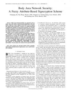
TABLE I. THE INDEX DATA OF NETWORK SECURITY FUZZY EVALUATION

The goal

The criterion level

Temperature, humidity and cleanliness control Fire prevention measures

A1 (0.33)

Power supply

(0.2, 0.6, 0.2, 0.0, 0.0) (0.5, 0.5, 0.0, 0.0, 0.0)

B12 (0.13)

(0.6, 0.4, 0.0, 0.0, 0.0)

B13 (0.09)

Lightning prevention measures Anti-static measures

(C1, C2, C3, C4, C5)

B11 (0.07)

Surrounding room environment

Physical security

Membership vectors

The factor level

(0.3, 0.6, 0.1, 0.0, 0.0)

B14 (0.13)

(0.7, 0.3, 0.0, 0.0, 0.0)

B15 (0.11)

(0.9, 0.1, 0.0, 0.0, 0.0)

B16 (0.13)

Free-standing equipment on ground and desk fixed measures Heart touching settings

(0.0, 0.3, 0.6, 0.1, 0.0)

B17 (0.11)

(0.1, 0.6, 0.2, 0.1, 0.0)

B18 (0.08)

Network security fuzzy evaluation

Servers, backbone equipment and lines backup strategies B19 (0.15)

(0.1, 0.5, 0.4, 0.0, 0.0)

Backup of important data

(0.6, 0.4, 0.0, 0.0, 0.0)

B21 (0.09)

(0.3, 0.5, 0.2, 0.0, 0.0)

System security audit

Logical security

A2 (0.46)

B22 (0.08) System operation log B23 (0.06)

(0.0, 0.2, 0.7, 0.1, 0.0)

Data recovery mechanism

(0.0, 0.1, 0.2, 0.5, 0.2)

Data encryption

(0.8, 0.2, 0.0, 0.0, 0.0)

B25 (0.13)

Information system access control mechanisms System software security

S

B24 (0.06)

Anti-hacking measures Anti-virus measures

(0.2, 0.6, 0.2, 0.0, 0.0)

B27 (0.14)

(0.0, 0.3, 0.4, 0.3, 0.0)

B28 (0.17)

(0.4, 0.4, 0.2, 0.0, 0.0)

B29 (0.17)

Information management security sector leaders and organization Information security system Management security

A3 (0.21)

(0.4, 0.5, 0.1, 0.0, 0.0) (0.2, 0.4, 0.3, 0.1, 0.0)

B33 (0.19)

Equipment and data management system completeness Registration file system

(0.9, 0.1, 0.0, 0.0, 0.0)

B31 (0.08)

B32 (0.12)

Information security personnel training measures

(0.6, 0.4, 0.0, 0.0, 0.0)

B34 (0.12)

(0.9, 0.1, 0.0, 0.0, 0.0)

B35 (0.11)

Anti-theft and anti-loss measures B 36 (0.10)

(0.0, 0.0, 0.2, 0.6, 0.2)

Password management security system

(0.3, 0.3, 0.4, 0.0, 0.0)

Accident emergency plan

B37 (0.17)

(0.6, 0.3, 0.1, 0.0, 0.0)

B38 (0.11)

IV. FUZZY EVALUATION ON NETWORK SECURITY BASED ON M(1,2,3) A. Network Security Fuzzy Evaluation Matrix According to Ref. [1], we can the network security fuzzy evaluation matrix in some organization, as Table I shows. In Table I, the values in brackets behind corresponding indexes are their importance weights; the vectors behind the base indexes are their membership vectors including five grades: C1 (very good), C2 (good), C3 (general), C4 (bad), and C5 (very bad). The data in the table are from Ref. [1].

© 2009 ACADEMY PUBLISHER

(0.6, 0.3, 0.1, 0.0, 0.0)

B26 (0.10)

B.

Fuzzy Evaluation Steps Based on M(1,2,3) Model 1) Calculating the membership vector of physical security A1 :

① A1 includes nine base indexes B11 ~ B19 , the evaluation matrix is: ⎛ ⎜ ⎜ ⎜ ⎜ ⎜ ⎜ U ( A1 ) = ⎜ ⎜ ⎜ ⎜ ⎜ ⎜⎜ ⎝

0.2 0.5 0.6 0.3 0.7 0.9 0.0 0.1 0.1

0.6 0.5 0.4 0.6 0.3 0.1 0.3 0.6 0.5

0.2 0.0 0.0 0.1 0.0 0.0 0.6 0.2 0.4

0.0 0.0 0.0 0.0 0.0 0.0 0.1 0.1 0.0

0.0 0.0 0.0 0.0 0.0 0.0 0.0 0.0 0.0

⎞ ⎟ ⎟ ⎟ ⎟ ⎟ ⎟ ⎟ ⎟ ⎟ ⎟ ⎟ ⎟⎟ ⎠

JOURNAL OF NETWORKS, VOL. 4, NO. 5, JULY 2009

329

According to the j th row ( j = 1 ~ 9) of U ( A1 ) , the distinguishable weights of B1 j are obtained and the

② In Table I, the importance weight vector of B21 ~ B29 is given:

distinguishable weight vector is:

β ( A2 ) = ( 0.09 0.08 0.06 0.06 0.13 0.10 0.14 0.17 0.17 )

α ( A1 ) = (0.0890 0.1237 0.1265 0.0961 0.1349 0.1735 0.0961 0.0703 0.0900)

② In Table I, the importance weight vector of B11 ~ B19 is given: β ( A1 ) = ( 0.07 0.13 0.09 0.13 0.11 0.13 0.11 0.08 0.15 )

Calculate the K th comparable value of ( j = 1,2 L 9) and obtain the comparable value matrix

③ B1 j

N ( A1 ) of A1 : ⎛ ⎜ ⎜ ⎜ ⎜ ⎜ ⎜ N ( A1 ) = ⎜ ⎜ ⎜ ⎜ ⎜ ⎜⎜ ⎝

0.0012 0.0037 0.0012

0

0.0080 0.0080 0.0068 0.0046

0 0

0 0

0.0037 0.0075 0.0012 0.0104 0.0045 0

0 ⎞ ⎟ 0 ⎟ 0 ⎟ ⎟ 0 ⎟ ⎟ 0 ⎟ 0 ⎟ ⎟ 0 ⎟ 0 ⎟ ⎟ 0 ⎟⎠

0 0

0.0203 0.0023 0 0 0 0.0032 0.0063 0.0011 0.0006 0.0034 0.0011 0.0006 0.0013 0.0067 0.0054 0

④ According to N ( A1 ) , calculate the K th comparable sum of A1 and obtain the comparable sum vector: M ( A1 ) = (0.0525 0.0438 0.0154 0.0016

0)

⑤ According to M ( A1 ) , calculate the membership vector μ ( A1 ) of A1 : μ ( A1 ) = ( 0.4631 0.3870 0.1356 0.0143

0)

2) Calculating the membership vector of logical security A2 : ① A2 includes nine base indexes B21 ~ B29 , the evaluation matrix is: ⎛ ⎜ ⎜ ⎜ ⎜ ⎜ ⎜ U ( A2 ) = ⎜ ⎜ ⎜ ⎜ ⎜ ⎜⎜ ⎝

0.6 0.3 0.0 0.0 0.8 0.6 0.2 0.0 0.4

0.4 0.5 0.2 0.1 0.2 0.3 0.6 0.3 0.4

0.0 0.2 0.7 0.2 0.0 0.1 0.2 0.4 0.2

0.0 0.0 0.1 0.5 0.0 0.0 0.0 0.3 0.0

0.0 0.0 0.0 0.2 0.0 0.0 0.0 0.0 0.0

⎞ ⎟ ⎟ ⎟ ⎟ ⎟ ⎟ ⎟ ⎟ ⎟ ⎟ ⎟ ⎟⎟ ⎠

According to the j th row ( j = 1 ~ 9) of U ( A2 ) , the distinguishable weights of B 2 j are obtained and the distinguishable weight vector is: α ( A2 ) = (0.1494 0.0925 0.1289 0.0620 0.1770 0.1135 0.1052 0.0831 0.0885)

© 2009 ACADEMY PUBLISHER

③

Calculate the K th comparable value of and obtain the comparable value

( j = 1,2 L 9) matrix N ( A2 ) of B2 j

⎛ ⎜ ⎜ ⎜ ⎜ ⎜ ⎜ N ( A2 ) = ⎜ ⎜ ⎜ ⎜ ⎜ ⎜⎜ ⎝

A2 :

⎞ ⎟ ⎟ ⎟ ⎟ 0 0.0004 0.0007 0.0019 0.0007 ⎟ ⎟ 0.0184 0.0046 0 0 0 ⎟ 0.0068 0.0034 0.0011 0 0 ⎟ ⎟ 0.0029 0.0088 0.0029 0 0 ⎟ 0 0.0042 0.0056 0.0042 0 ⎟ ⎟ 0.0060 0.0060 0.0030 0 0 ⎟⎠ 0.0081

0.0054

0

0

0

0.0022 0.0037 0.0015 0 0.0015 0.0054 0.0008 0

0 0

④ According to N ( A2 ) , calculate the K th comparable sum of A2 and obtain the comparable sum vector: M ( A2 ) = (0.0445 0.0381 0.0204 0.0069 0.0007)

⑤ According to M ( A2 ) , calculate vector μ ( A2 ) of A2 :

the membership

μ ( A2 ) = (0.4022 0.3446 0.1843 0.0621 0.0067)

3) Calculating the membership vector of management security A3 ① A3 includes eight base indexes B31 ~ B38 , the evaluation matrix is: ⎛ ⎜ ⎜ ⎜ ⎜ ⎜ U ( A3 ) = ⎜ ⎜ ⎜ ⎜ ⎜ ⎜ ⎝

0.9 0.4 0.2 0.6 0.9 0.0 0.3 0.6

0.1 0.5 0.4 0.4 0.1 0.0 0.3 0.3

0.0 0.1 0.3 0.0 0.0 0.2 0.4 0.1

0.0 0.0 0.1 0.0 0.0 0.6 0.0 0.0

0.0 0.0 0.0 0.0 0.0 0.2 0.0 0.0

⎞ ⎟ ⎟ ⎟ ⎟ ⎟ ⎟ ⎟ ⎟ ⎟ ⎟ ⎟ ⎠

According to the j th row ( j = 1 ~ 8) of U ( A3 ) , the distinguishable weights of B3 j are obtained and the distinguishable weight vector is: α ( A3 ) = (0.2009 0.1042 0.0516 0.1465 0.2009 0.1031 0.0814 0.1113)

② In Table I, the importance weight vector of B31 ~ B38 is given:

β ( A3 ) = ( 0.08 0.12 0.19 0.12 0.11 0.10 0.17 0.11 )

330

JOURNAL OF NETWORKS, VOL. 4, NO. 5, JULY 2009

③ Calculate the K th comparable value of B3 j ( j = 1,2 L 9) and obtain the comparable value

matrix N ( A3 ) of A3 : ⎛ ⎜ ⎜ ⎜ ⎜ ⎜ N ( A3 ) = ⎜ ⎜ ⎜ ⎜ ⎜ ⎜ ⎝

0

0

the confidence degree is no lower than

k ∑ μt t =1

(S ) .

In the example, according to the final membership vector μ (S ) , we can judge that S belongs the C2 (good), with the confidence degree 80.21%(0.4594+ 0.3427= 0.8021). In the Ref. [1], the final membership vector of network security evaluation is:

⎞ ⎟ 0.0050 0.0063 0.0013 0 0 ⎟ 0.0020 0.0039 0.0029 0.0010 0 ⎟ ⎟ 0.0105 0.0070 0 0 0 ⎟ ⎟ 0.0199 0.0022 0 0 0 ⎟ 0 0 0.0021 0.0062 0.0021⎟ ⎟ 0.0042 0.0042 0.0055 0 0 ⎟ 0.0073 0.0037 0.0012 0 0 ⎟⎠ 0.0145 0.0016

And judge that S belongs the K k th grade, of which

0

μ (S ) = (μ1 (S ),..., μ 5 (S ))

= (0.38270 0.34794 0.18796 0.06956 0.01184 )

④ According to N ( A3 ) , calculate the K th comparable sum of A3 and obtain the comparable sum vector:

The judgment result is the same C2 (good), but the confidence degree is only 73.064% (0.38270+0.34794 =0.73064).

M ( A3 ) = (0.0634 0.0288 0.0130 0.0072 0.0021)

V. CONCLUSIONS

⑤ According to M ( A3 ) , calculate the membership vector μ ( A3 ) of A2 :

The transformation of membership degree is the key computation of fuzzy evaluation for multi-indexes fuzzy decision-making, but the existing transformation methods have some questions. The paper analyzes the reasons of the questions, obtains the solving method, and at last builds the M (1, 2, 3) model without the interference of

μ ( A3 ) = (0.5536 0.2520 0.1137 0.0626 0.0180)

4) Network security comprehensive evaluation matrix U (S ) From the above three steps, we can get network security comprehensive evaluation matrix U (S ) : ⎛ μ ( A1) ⎞ ⎜ ⎟ U (S ) = ⎜ μ ( A2 ) ⎟ ⎜ μ(A ) ⎟ 3 ⎠ ⎝ 0 ⎛ 0.4631 0.3870 0.1356 0.0143 ⎜ = ⎜ 0.4022 0.3446 0.1843 0.0621 0.0067 ⎜ 0.5536 0.2520 0.1137 0.0626 0.0180 ⎝

⎞ ⎟ ⎟ ⎟ ⎠

In Table I, the importance weight vector of B1 ~ B3 is given:

β (S ) = ( 0.33 0.46 0.21

)

So we can calculate the final membership vector

μ (S ) of the goal S :

μ (S ) = (μ1 (S ),..., μ 5 (S ))

= (0.4594 0.3427 0.1492 0.0424 0.0063)

C. Network Security Recognition Because the classification of network security evaluation grades is orderly, that is, C k is superior to C k +1 , so we apply confidence recognition rule to determine the grade of network security. Let λ (λ > 0.7 ) is the confidence, calculate ⎧ k ⎫ K 0 = min ⎨k ∑ μ t (S ) ≥ λ ,1 ≤ k ≤ 5⎬ . ⎩ t =1 ⎭

© 2009 ACADEMY PUBLISHER

+) and is a redundant data, which is different from M (•, 　 nonlinear model. M (1, 2, 3) provides the general method for membership transformation of multi–indexes decisionmaking in application fields. The theory value is that it provides transformation method which is comply to logics to realize the transformation universe fuzzy set to universe fuzzy set in fuzzy logical system. From index membership degree of base level, after obtain one index membership degree vector in adjacent upper level by M (1,2,3) , thus, by the same computation, obtaining membership degree vector of top level. Because of normalization of computation, M (1,2,3) is suitable for membership transformation which contains multi-levels, multi-indexes, large data. Security is a very difficult topic. Everyone has a different idea of what “security”' is, and what levels of risk are acceptable. The key for building a secure network is to take preventive measures to solve network security problems and minimize various network security threats, so it is essential to evaluate network system security in advance. The paper applies the new algorithm in the fuzzy evaluation on network security and example results also prove that M (1, 2, 3) can improve the evaluation accuracy and credibility.

REFERENCES [1] Zhang Xihai., “The Application of Fuzzy Comprehensive Evaluation for Network Security Evaluation”, Nanjing University of Technology and Engineering, 2006. [2] Zadeh L.A., "Fuzzy sets", Information and Control, 1965(8), pp.338–353.

JOURNAL OF NETWORKS, VOL. 4, NO. 5, JULY 2009

[3] LI Feng qi, XIE Jun, LI,Yao, “New Methods of Fitting the Membership Function of Oceanic Water Masses”, Periodical of Ocean University of China , 2004.1, pp.1-9. [4] Jun Chen, Susan Bridges, Julia Hodges, “Derivation of Membership Functions for Fuzzy Variables Using Genetic Algorithms”, 1998. [5] http://en.wikipedia.org/wiki/Membership_function_(mathe matics) [6] QIN Shou-kang et, The Theory and Application of Comprehensive Evaluation, Beijing: electronic industry publishing house, 2003, pp.124. [7] WANG You-qiang, CHEN Shun-qing, HUANG Bing-xi, “The Reliability Study of Colliery Machine Components”, Colliery Machine, 2004, (2), pp.53-55. [8] LV Ying-zhao, HE Shuan-hai, “The Fuzzy Reliability Evaluation for Defect Reinforced Concrete on Bridges”, Journal of Traffic and Transportation Engineering, 2005, 5(4), pp.58-62. [9] HU Sheng-wu, LI Chang-chun, WANG Xin-zhou, “GIS Quality Comprehensive Assessment Based on Multi-level Fuzzy Evaluation”, Journal of Yangtze River Scientific research, 2005, 22(3), pp.21-23. Xian-bin, CHEN Guo-ming, “Fuzzy [10] ZHENG Comprehensive Evaluation Research Based on FTA Oil and Gas Transport Vessel”, Systems Engineering—Theory & Practice, 2005, (2), pp.139-1144. [11] LI Hai-ling, LIU Ke-jian,LI Qian, “The Research of Fuzzy Comprehensive Evaluation for Project Risk”, Journal of XI Hua University, 2004, 24(6), pp.78-81. [12] HUANG Yu-kun, CUI Xin-yuan, JIA Sa-sa, “Fuzzy Comprehensive Evaluation Research for Project”, Journal ZHE Jiang transportation college, 2005,6(4), pp.1-5. [13] HUANG Guang-long, YU Zhong-hua, Wu Zhao-tong, “Subject-Object Comprehensive Evaluation Based on Evidence Reasoning and Rough Set Theory”, China Mechanical Engineering, 2001, 12(8), pp:930-934. [14] GUO Jie, HU Mei-xin, “The Improvement of Fuzzy Evaluation Research for Project Risk”, Industrial Engineering Journal, 2007, 10(3), pp.86-90. [15] Jianwei Han, Micheline, Data Mining: Concepts and Techniques, CA: Morgan Kaufman Publisher, 2000. [16] JIA Lin, LI Ming, “The Losing Model of Customers of Telecom Based on Data Mining”, Computer Engineering and Aapplication, 2004, pp.185-187. [17] YANG Wen-xian, REN Xing-min, QIN Wei-yang, “Research of Complex Equipment Fault Diagnosis Method”, Journal of Vibration Engineering, 2000, 13(5), pp. 48-51.

© 2009 ACADEMY PUBLISHER

331

[18] Zhang Weiqun., “A Review and Forecast of the Study and Application of Data Digging”, Statistics & Information Forum, 2004, 19(1):,pp. 95-96. [19] Gao Yilong, “Data Mining and Its Application in Engineering Diagnosis”, Xi'an Jiaotong University, 2000. [20] Liu Kai-Di, Pang Yan-Jun, Hao Ji-Mei, “The Improved Algorithm of Fuzzy Comprehensive Evaluation for Vendor Selection of Iron and Steel Enterprises”,. Statistics and Decision, 2008(16), pp.171-173.

Hua. Jiang, born in 1977-1-9, Handan, Hebei Province, China. In March, 2006, graduated from Hebei University of Engineering and obtained postgraduate qualifications. Main research fields: network security, information management, supply chain management. Now works in Information Management Department, Economics and Management School, Hebei University of Engineering, Lecturer. Mainly published articles: Jiang, Hua, “Study on mobile E-commerce security payment system”, Proceedings of the International Symposium on Electronic Commerce and Security, ISECS 2008, Aug 3-5 2008, pp.754-757; Jiang Hua, Ruan Junhu, “Analysis of Influencing Factors on Performance Measurement of the Supply Chain Based on SCOR-model and AHM”, IEEE/SOLI'2008; Beijing, China October 12-15, 2008, pp.2141-2146; Xiaofeng Zhao, Hua Jiang, Liyan Jiao, “A Data Fusion Based Intrusion Detection Model”, International Symposium on Education and Computer Science (ECS2009), 7-8 March, 2009 Wuhan, Hubei, China (in press). Current research interests: management optimization and scientific decision-making. Junhu. Ruan, born in 1983-10-12, Zhoukou, Henan Province, China. Postgraduate of Hebei University of Engineering. Main research fields: logistic and supply chain management, scientific evaluation and prediction. Published article: Jiang Hua, Ruan Junhu, “Analysis of Influencing Factors on Performance Measurement of the Supply Chain Based on SCOR-model and AHM”, IEEE/SOLI'2008; Beijing, China October 12-15, 2008, pp.2141-2146. Current research interests: scientific evaluation and combined forecasting.