(IJCSIS) International Journal of Computer Science and Information Security,. Vol. 6, No. 3, 2009 ... Keywords: fuzzy set theory, fuzzy linear programming, logistic membership ..... He has a Bachelor's Degree in Mechanical. Engineering from ...
(IJCSIS) International Journal of Computer Science and Information Security, Vol. 6, No. 3, 2009
Application of a Fuzzy Programming Technique to Production Planning in the Textile Industry J. F. Webb
*I. Elamvazuthi , T. Ganesan, P. Vasant
Swinburne University of Technology Sarawak Campus, Kuching, Sarawak, Malaysia
Universiti Technologi PETRONAS Tronoh, Malaysia *
analysis of real-world problems [3]. The period of development of fuzzy theory from 1965 to 1977, is often referred to as the academic phase. The outcome was a rather small number of publications of a predominantly theoretical nature by a few contributors, mainly from the academic community. At this time, not much work in the area of fuzzy decision making was reported. The period from 1978 to 1988, has been called the transformation phase during which significant advances in fuzzy set theory were made and some real-life problems were solved. In this period, some important principles in fuzzy set theory and its applications were established. However, work on fuzzy decision making was not very active, in the area of engineering applications. Some earlier work on fuzzy decision making can be found in [4] and [5]. From 1989 to the present work on fuzzy techniques has boomed . In this period, many problems concerning applications in industry and business have been tackled successfully. In the early 1990s, fuzzy techniques were used to aid the solution of some soft computing problems. The aim of soft computing is to exploit, whenever possible, the tolerance for imprecision and uncertainty in order to achieve computational tractability, robustness, and low cost, by methods that produce approximate but acceptable solutions to complex problems which often have no precise solution.
Abstract—Many engineering optimization problems can be considered as linear programming problems where all or some of the parameters involved are linguistic in nature. These can only be quantified using fuzzy sets. The aim of this paper is to solve a fuzzy linear programming problem in which the parameters involved are fuzzy quantities with logistic membership functions. To explore the applicability of the method a numerical example is considered to determine the monthly production planning quotas and profit of a home-textile group. Keywords: fuzzy set theory, fuzzy linear programming, logistic membership function, decision making
I.
INTRODUCTION
Many problems in science and engineering have been considered from the point of view optimization. As the environment is much influenced by the disturbance of social and economic factors, the optimization approach is not always the best. This is because, under such turbulent conditions, many problems are ill-defined. Therefore, a degree-of-satisfaction approach may be better than optimization. Here, we discuss how to deal with decision making problems that are described by fuzzy linear programming (FLP) models and formulated with elements of imprecision and uncertainty. More precisely, we will study FLP models in which the parameters are known only partially to some degree of precision.
Currently, fuzzy techniques are often applied in the field of decision making. Fuzzy methods have been developed in virtually all branches of decision making, including multiobjective, multi-person, and multi-stage decision making [6]. Apart from this, other research work connected to fuzzy decision making includes applications of fuzzy theory in management, business and operational research [7]. Some representative publications can be found in [8], [9], [10], [11] and [12].
Even though the information is incomplete, the model builder is able to provide realistic intervals for the parameters in these FLP models. We will demonstrate that the modeling complications can be handled with the help of some results which have been developed in fuzzy set theory. The FLP problem which we will be considering in this work is to find ways to handle fuzziness in the parameters. We will develop a FLP model in which the parameters are known with only some degree of precision. We will also show that the model can be parameterized in such a way that a satisfactory solution becomes a function of the membership values. The FLP model derived in this way is flexible and easy to handle computationally [1].
Decision making is an important and much studied application of mathematical methods in various fields of human activity. In real-world situations, decisions are nearly always made on the basis of information which, at least in part, is fuzzy in nature. In some cases fuzzy information is used as an approximation to more precise information. This form of approximation can be convenient and sufficient for making good enough decisions in some situations. In other cases, fuzzy information is the only form of information available.
The first and most meaningful impetus towards the mathematical formalization of fuzziness was pioneered by Zadeh [2]. Its further development is in progress, with numerous attempts being made to explore the ability of fuzzy set theory to become a useful tool for adequate mathematical
238
http://sites.google.com/site/ijcsis/ ISSN 1947-5500
The first step in mathematically tackling a practical decision-making problem consists of formulating a suitable mathematical model of a system or situation. If we intend to make reasonably adequate mathematical models of situations that help practicing decision makers in searching for rational decisions, we should be able to introduce fuzziness into our models and to suggest means of processing fuzzy information. In this paper a methodology to solve an FLP problem by using a logistic membership function is considered. The rest of the paper is organized as follows. In section 2, the basic fuzzy model is defined and this is followed by a numerical example in section 3. Section 4 provides the results and discussion, and finally, concluding remarks are made in section 5. II.
μa%ij
III.
THE MODEL
Maximize Cx Ax ≤ b, x ≥ 0.
(1)
in which the components of a 1×n vector C, an m×n matrix A and an n×1 vector b are all crisp parameters and x is an ndimensional decision variable vector. The system (1) may be redefined in a fuzzy environment with the following more elaborate structure: n
Maximize
if aija ≤ aij ≤ aijb
(4)
if aij ≥ aijb
NUMERICAL EXAMPLE
TABLE I. REQUIRED PROCESS TIME FOR SHEET, PILLOW CASE AND OF A QUILT [14]
∑cjxj ~
j =1
Departments
Subject to n
if aij ≤ aija
In this example the profit for a unit of sheet sales is around 1.05 Euro; a unit of pillow case sales is around 0.3 Euro and a unit of quilt sales is around 1.8 Euro. The firm concerned would like to sell approximately 25.000 sheet units, 40.000 pillow case units and 10.000 units quilt units. The monthly working capacity and required process time for the production of sheets, pillow cases and quilts are given in Table 1 [14]. In view of this, let us determine monthly production planning details and profit for a home-textile group. X1 presents the quantity of sheets that will be produced, X2 presents the quantity of pillow cases and X3 presents the quantity of quilts. The profit figures with logistic membership functions as given in Table I.
A conventional linear programming problem is defined by
Subject to
⎧ ⎪ ⎪1 ⎪⎪ B =⎨ ⎛ aij − aija ⎞ α⎜ b a ⎟ ⎪ ⎜ ⎟ ⎪ 1 + Ce ⎝ aij − aij ⎠ ⎪ ⎪⎩ 0
∑ aij x j ≤~ bi , ~
j =1
i = 1,2 L m
Cutting Sewing Pleating Packaging
(2)
~ a b ~ a b ~ ~ All fuzzy data c j ≡ S (c j , c j ) and aij ≡ S (aij , aij ) are fuzzy variables with the following logistic membership functions [13], ⎧ ⎪ ⎪1 ⎪ B ⎪ μc% j = ⎨ ⎛ c j −caj ⎞ ⎪ α⎜ b a ⎟ ⎜ c j −c j ⎟ ⎪ ⎝ ⎠ ⎪ 1+ Ce ⎪0 ⎩
Required unit time(hour) Sheet
Pillow case
Quilt
Working hours per month
0.0033 0.056 0.0067 0.01
0.001 0.025 0.004 0.01
0.0033 0.1 0.017 0.01
208 4368 520 780
If we consider, around 1.05 ≡ S% (1.02,1.08) , around 0.3 ≡ S% (0.2, 0.4) , and around 1.8 ≡ S% (1.7, 2.0) , then, the mathematical model of the above problem with fuzzy objective coefficients can be described as follows.
if c j ≤ caj if caj ≤ c j ≤ cbj
Maximize ~ ~ ~ S (1.02,1.08) x1+ S (0.2,0.4) x 2 + S (1.7, 2.0) x 3
(3)
subject to 0 . 033 x1 + 0 . 01 x 2 + 0 .0033 x 3 ≤ 208 ;
if c j ≥ cbj
0 . 056 x1 + 0 .25 x 2 + 0 .1 x 3 ≤ 4368 ; 0 . 0067 x1 + 0 .04 x 2 + 0 .17 x 3 ≤ 520 ; 0 . 1 x1 + 0 . 1 x 2 + 0 .01 x 3 ≤ 780 ; x1 ≥ 25000 ; x 2 ≥ 40000 ; x 3 ≥ 10000 ;
239
http://sites.google.com/site/ijcsis/ ISSN 1947-5500
(5)
and we set
B = 1, C = .001, ε = 0.2 and d = 13.8 [15].
The aspiration of the objective function is calculated by solving the following: Maximize
1.08 x 1 +0.4 x2 + 2.0 x3
subject to .0033x1 + .001x2 + .0033 x3 ≤ 208; .056 x1 + .025 x2 + .1x3 ≤ 4368; .0067 x1 + .004 x2 + .017 x3 ≤ 520;
(6)
.01x1 + .01x2 + .01x3 ≤ 780; x1 ≥ 25000; Figure 1. 3D plot for iterations M=748.
x2 ≥ 40000; x3 ≥ 10000;
Fig. 2 shows the 3D outcome for M = 749 iterations and various alpha values with respect to G. The optimum values for the objective function as per this figure are 86,691.8 (maximum) and 86,639.5 (minimum).
which gives the optimal value of the objective function as 67203.88 for x1 = 29126.21, x2 =35000.00 and x3 =10873.79 [15]. With the help of the program LINGO version 10.0 we obtain the following results [15]: λ = 0.5323011, x1 = 27766.99, x2 = 40000.00, x3 = 10233.01, η = 0.4911863
Therefore, to achieve maximum profit the home-textile group should plan for a monthly production of 27766.99 sheet units, 40000 pillow case units and 102333.01 quilt units. This plan gives an overall satisfaction of 0.5323011. The decision making method may be improved further by adopting a recursive iteration methodology. IV.
Figure 2. 3D plot for iterations M = 749.
RESULTS AND DISCUSSION
Fig. 3 shows the 3D outcome for M = 750 iterations and various alpha values with respect to G. The optimum values for the objective function as per this figure are 86,576.2 (maximum) and 86,524.0 (minimum).
The numerical example is solved by using a recursive method for various iterations. This was carried out using the C++ programming language on a personal computer with a dual core processor running at 2 GHz [16]–[17]. Fig. 1 shows the 3D outcome of the iterations with M = 748 for various alpha values with respect to the objective function G. The values of α 1 and α 2 vary from 0 to 1. The optimum values for the objective function as per Fig. 1 are 86,807.7 (maximum) and 86,755.4 (minimum).
Figure 3. 3D plot for iterations M=750.
240
http://sites.google.com/site/ijcsis/ ISSN 1947-5500
Fig. 4 shows the 3D outcome for M = 751 iterations and various alpha values with respect to G. The optimum value for the objective function as per this figure are 86,440.7 (maximum) and 86,408.0 (minimum).
Figure 6. Decision variable, X1 versus M iterations.
Figure 4. 3D plot for iterations M=751.
Fig. 5 shows the linear approximation for G with respect to iterations 748 to 751. It can be seen that as the iterations are increased, the values of the objective function decrease. The percentage error is minimum at iteration, M = 748; however, after that it increases until it peaks at M = 750; thereafter, the percentage error decreases again to a level lower than that at M = 748. This shows that the maximum number of iterations that can be used for similar cases in the future can be limited to M = 750. Figure 7. Decision variable, X2 versus M iterations.
Figure 8. Decision variable, X2 versus M iterations. Figure 5. Objective Function (G) versus iterations
Table II presents results that involve
Figs. 6, 7 and 8 show the linear approximation for the decision variables x1, x2 and x3 with respect to the number of iterations. It can be observed that x1, x2 and x3 decrease as the iterations are increased from M = 748 to M = 751.
α1 , α 2
and
α3
with M
= 748 for G, x1, x2 and x3. Other results for M = 749 to 751 are given in the appendix.
241
http://sites.google.com/site/ijcsis/ ISSN 1947-5500
From Table IV, the optimum value for the objective function using the proposed method outweighs the results obtained in [14] and [15]. It can be deduced that the recursive iteration method proposed here is an efficient and effective way to solve our example fuzzy problem of production planning in the textile industry.
TABLE II ALPHA, OBJECTIVE FUNCTION AND DECISION VARIABLES FOR M=748 α1
α2
α3
G
x1
x2
x3
1
1
*all
86755.4
33422.5
53475.9
1
0.5
all
86780.3
33422.5
53475.9
13369 13369
0.5
1
all
86767.5
33422.5
53475.9
13369
0.5
0.5
all
86792.4
33422.5
53475.9
13369
0.3333
1
all
86770.9
33422.5
53475.9
13369
0.3333
0.5
all
86795.9
33422.5
53475.9
13369
0.25
1
all
86772.5
33422.5
53475.9
13369
0.25
0.5
all
86797.5
33422.5
53475.9
13369
0.2
1
all
86773.5
33422.5
53475.9
13369
0.2
0.5
all
86798.4
33422.5
53475.9
13369
0.1667
1
all
86774.1
33422.5
53475.9
13369
0.1667
0.5
all
86799.0
33422.5
53475.9
13369
0.1429
1
all
86774.5
33422.5
53475.9
13369
0.1429
0.5
all
86799.4
33422.5
53475.9
13369
0.125
1
all
86774.8
33422.5
53475.9
13369
0.125
0.5
all
86799.8
33422.5
53475.9
13369
0.1111
1
all
86775.1
33422.5
53475.9
13369
0.1111
0.5
all
86800.0
33422.5
53475.9
13369
V.
This paper has discussed the use of fuzzy linear programming for solving a production planning problem in the textile industry. It can be concluded that the recursive method introduced is a promising method for solving such problems. The modified s-curve membership function provides various uncertainty levels which are very useful in the decision making process. In this paper, only a single s-curve membership function was considered. In the future, various other membership functions will be considered. Apart from providing an optimum solution for the objective functions, the proposed method ensures high productivity. In this regard, there is a good opportunity for developing an interactive selforganized decision making method by using hybrid soft computing techniques. ACKNOWLEDGMENT The authors would like to thank Universiti Teknologi PETRONAS and Swinburne University of Technology Sarawak Campus for supporting this work.
Note: *all∈ (0, 1) Table III summarizes the result for M = 748 to 751 for x1, x2 and x3 with maximum and minimum values of G. The overall maximum value for G is 86807.7 at M = 748 and the overall minimum value is 86408.0 at M = 751.
REFERENCES [1] [2] [3]
TABLE III SUMMARY OF ITERATIONS, DECISION VARIABLES AND OBJECTIVE FUNCTION M
x1
x2
x3
G (max)
G(min)
748
33422.5
53475.9
13369
86807.7
86755.4
749
33377.8
53404.5
13351.1
86691.8
86639.5
750
33333.3
53333.3
13333.3
86576.2
86524.0
[6]
751
33288.9
53262.3
13315.6
86440.7
86408.0
[7]
[4] [5]
Table IV compares the best objective function and decision variables x1, x2 and x3 of the proposed method with previous work by other researchers.
[8] [9] [10]
TABLE IV COMPARATIVE ANALYSIS
[11]
The Best Objective Function
x1
x2
x3
Irfan [14]
64390.999
33825.16
40000.00
9374.760
Atanu [15]
66454.369
27766.99
40000.00
10233.01
Proposed Method
86807.700
33422.50
53475.90
13369.00
Method
CONCLUSION
Decision Variables
[12] [13]
242
Delgado, M., Verdegay, J.L. and Vila, M. A. 1989. A General Model For Fuzzy Linear Programming. Fuzzy Sets and Systems 29 : 21-29. Zadeh, L. A. 1965. Fuzzy sets. Information and Control 8 : 338-353. Orlovsky, S. A. 1980. On Formalization Of A General Fuzzy Mathematical Programming Problem. Fuzzy Sets and Systems 3 : 311321. Kickert, W.J. 1978. Fuzzy Theories on Decision-Making: Frontiers in Systems Research. Leiden, The Netherlands : Martinus Nijhoff . Zimmermann, H.J. 1987. Fuzzy Sets, Decision Making, and Experts Systems. Boston: Kluwer. Tamiz, M. 1996. Multi-objective programming and goal programming: theories and applications. Germany: Springer-Verlag. Zimmermann, H.J. 1991. Fuzzy Set Theory-and Its Applications, (2nd rev. ed.). Boston: Kluwer. Ross, T. J. 1995. Fuzzy Logic with Engineering Applications, New York: McGraw- Hill. Klir, G. J., and Yuan, B. 1995. Fuzzy Sets and Fuzzy Logic: Theory and Applications. Upper Saddle River, NJ: Prentice Hall PTR. Yager, R. R., Ovchinikov,S., Tong, R. M., Nguyen,H. T (eds.) 1987. Fuzzy Sets and Applications-Selected Papers by L. A. Zadeh. New York :John Wiley. Zimmermman, H. J. 1985. Application of Fuzzy Set Theory To Mathematical Programming. Information Sciences 36:25-58. Dubois, D. and Prade, H.1980. Fuzzy Sets and Systems, Theory and Applications, California: Academic Press Inc. P. Vasant, A. Bhattacharya, B. Sarkar and S. K. Mukherjee, “Detection of level of satisfaction and fuzziness patterns for MCDM model with modified flexiable S-curve MF”, Applied Soft Computing, 7, 2007, pp. 1044-1054.
http://sites.google.com/site/ijcsis/ ISSN 1947-5500
[14] Irfan Ertugrul and Aysegül Tus, “Interactive fuzzy linear programming and an application sample at a textile firm”, Fuzzy Optimization and Decision Making, 6, 2007, pp. 29–49. [15] Atanu, S., P. Vasant and Cvetko, J.A., Fuzzy Optimization with Robust Logistic Membership Function: A Case Study In For Home Textile Industry, Proceedings of the 17th World Congress, The International Federation of Automatic Control, Seoul, Korea, July6-11, 2008, pp52625266. [16] http://www.intel.com/products/processor/core2duo/index.htm [17] http://www2.research.att.com/~bs/C++.html
0.1667
1
all
86542.7
33333.3
53333.3
13333.3
0.1667
0.5
all
86567.5
33333.3
53333.3
13333.3
0.1429
1
all
86543.1
33333.3
53333.3
13333.3
0.1429
0.5
all
86568
33333.3
53333.3
13333.3
0.125
1
all
86543.4
33333.3
53333.3
13333.3
0.125
0.5
all
86568.3
33333.3
53333.3
13333.3
0.1111
1
all
86543.7
33333.3
53333.3
13333.3
0.1111
0.5
all
86568.5
33333.3
53333.3
13333.3
Note: *all∈ (0, 1)
APPENDIX
TABLE V II ALPHA, OBJECTIVE FUNCTION AND DECISION VARIABLES FOR M=751
TABLE V ALPHA, OBJECTIVE FUNCTION AND DECISION VARIABLES FOR M=749 α1
α2
α3
1
1
1
0.5
0.5
1
G
x1
x2
α1
x3
α2
α3
1
1
G
x1
x2
x3
*all
86408.8
33288.9
53262.3
13315.6
*all
86639.5
33377.8
53404.5
13351.1
all
86664.4
33377.8
53404.5
13351.1
1
0.5
all
86433.6
33288.9
53262.3
13315.6
13351.1
0.5
1
all
86420.9
33288.9
53262.3
13315.6
0.5
all
86445.7
33288.9
53262.3
13315.6 13315.6
all
86651.7
33377.8
53404.5
0.5
0.5
all
86676.6
33377.8
53404.5
13351.1
0.5
0.3333
1
all
86655.1
33377.8
53404.5
13351.1
0.3333
1
all
86424.3
33288.9
53262.3
13351.1
0.3333
0.5
all
86449.1
33288.9
53262.3
13315.6
1
all
86425.9
33288.9
53262.3
13315.6
0.3333
0.5
all
86680.0
33377.8
53404.5
0.25
1
all
86656.7
33377.8
53404.5
13351.1
0.25
0.25
0.5
all
86681.6
33377.8
53404.5
13351.1
0.25
0.5
all
86450.7
33288.9
53262.3
13315.6
1
all
86426.9
33288.9
53262.3
13315.6
0.5
all
86451.7
33288.9
53262.3
13315.6 13315.6
0.2
1
all
86657.6
33377.8
53404.5
13351.1
0.2
0.2
0.5
all
86682.5
33377.8
53404.5
13351.1
0.2
0.1667
1
all
86658.2
33377.8
53404.5
13351.1
0.1667
1
all
86427.5
33288.9
53262.3
13351.1
0.1667
0.5
all
86452.3
33288.9
53262.3
13315.6
1
all
86427.9
33288.9
53262.3
13315.6
0.1667
0.5
all
86683.1
33377.8
53404.5
0.1429
1
all
86658.7
33377.8
53404.5
13351.1
0.1429
0.1429
0.5
all
86683.5
33377.8
53404.5
13351.1
0.1429
0.5
all
86452.7
33288.9
53262.3
13315.6
0.125
1
all
86659.0
33377.8
53404.5
13351.1
0.125
1
all
86428.2
33288.9
53262.3
13315.6
0.125
0.5
all
86683.9
33377.8
53404.5
13351.1
0.125
0.5
all
86453
33288.9
53262.3
13315.6
0.1111
1
all
86428.4
33288.9
53262.3
13315.6
0.1111
0.5
all
86453.3
33288.9
53262.3
13315.6
0.1111
1
all
86659.2
33377.8
53404.5
13351.1
0.1111
0.5
all
86684.4
33377.8
53404.5
13351.1
Note: *all∈ (0, 1)
Note: *all∈ (0, 1) , M= no. of iterations
AUTHOR PROFILES TABLE VI ALPHA, OBJECTIVE FUNCTION AND DECISION VARIABLES FOR M=750 α1
α2
α3
1
1
1
0.5
0.5 0.5 0.3333 0.3333
*all
G
x1
x2
I. Elamvazuthi is a lecturer in the Department of Electrical and Electronic Engineering, Universiti Teknologi PETRONAS (UTP), Malaysia. His research interests include Control Systems, Mechatronics and Robotics. x3
86524
33333.3
53333.3
13333.3
all
86548.9
33333.3
53333.3
13333.3
1
all
86536.1
33333.3
53333.3
13333.3
0.5
all
86561
33333.3
53333.3
13333.3
1
all
86539.5
33333.3
53333.3
13333.3
0.5
all
86564.4
33333.3
53333.3
13333.3
0.25
1
all
86541.1
33333.3
53333.3
13333.3
0.25
0.5
all
86566
33333.3
53333.3
13333.3
0.2
1
all
86542.1
33333.3
53333.3
13333.3
0.2
0.5
all
86566.9
33333.3
53333.3
13333.3
T. Ganesan is currently a Graduate Assistant with the Department of Mechanical Engineering, Universiti Teknologi PETRONAS (UTP), Malaysia, pursuing a Masters Degree. He has a Bachelor’s Degree in Mechanical Engineering from the same university. He specializes in Computational Fluid Mechanics. P. Vasant is a lecturer in the Department of Fundamental and Applied Sciences, Universiti Teknologi PETRONAS (UTP), Malaysia. His research interests are Soft Computing and Computational Intelligence. J. F. Webb is a lecturer at Swinburne University of Technology, Sarawak Campus, Kuching, Sarawak, Malaysia. He specializes in Computational Methods, Nano-Physics and Ferroelectric Materials.
243
http://sites.google.com/site/ijcsis/ ISSN 1947-5500