Optimizing Linear Programming Technique Using Fuzzy Logic Sonja Petrovic-Lazarevic and Ajith Abraham* Monash University, Department of Management McMahons Road, Frankston 3199, Australia Email:
[email protected] *
Monash University, School of Computing and Information Technology, Gippsland campus, Churchill 3842, Australia, Email:
[email protected]
Abstract The purpose of this paper is to point to the usefulness of applying a linear mathematical formulation of fuzzy multiple criteria objective decision methods in organising business activities. In this respect fuzzy parameters of linear programming are modelled by preference-based membership functions. This paper begins with an introduction and some related research followed by some fundamentals of fuzzy set theory and technical concepts of fuzzy multiple objective decision models. Further a real case study of a manufacturing plant and the implementation of the proposed technique is presented. Empirical results clearly show the superiority of the fuzzy technique in optimising individual objective functions when compared to non-fuzzy approach. Furthermore, for the problem considered, the optimal solution helps to infer that by incorporating fuzziness in a linear programming model either in constraints, or both in objective functions and constraints, provides a similar (or even better) level of satisfaction for obtained results compared to non-fuzzy linear programming. Keywords: Fuzzy multiple objective decision making, business activities, degree of satisfaction, tolerances of fuzzy constraints.
1 Introduction Many years before the introduction of mathematical planning methods decision processes of organising business activities were based on intuition and experience. Decisions were subject to professional judgements usually based on imprecise information. Today business-planning processes in spite of the application of mathematical planning principles still utilise subjective judgements, making decisions often vague. Organising a business activity is a multiple objective
decision process. Since a decision is usually vague, it may be based on fuzzy numbers. In 1980 Dyson stated that fuzzy programming models should not be treated as a new contribution to multiple objective decision making methods, but rather as a lead to new conventional decision methods. ì Support for this thesis would require examples of new and affective fuzzy inspired multi-criteria methodsî [6]. The paper is an attempt to point to a significance of applying a fuzzy approach to multi objective decision methods in the process of organising business activities. In this respect the paper analyses the appropriateness of applying either the non-fuzzy multi objective decision model, with crisp objectives and fuzzy constraints, or the fuzzy multi objective decision model, with both fuzzy objectives and fuzzy constraints. The paper is organised as follows: next section covers a literature review of multi objective decision models. Section three contains definitions relevant to fuzzy set theory. Section four elaborates nonfuzzy multiple objective decision model (MODM) and the fuzzy MODM (FMODM) is explained in section five. The results of two models are presented in the case study of a construction firm that produces, transports and places concrete on construction sites. The paper ends with concluding remarks and future research directions.
2 Literature Review In real-world decision-making processes in business, decision making theory has become one of most important fields. It uses the optimisation methodology connected with a single criterion, but also satisfying concepts of multiple criteria. Decision processes with multiple criteria deal with human judgement. This is not easy to model. The human judgement element is in the area of preferences defined by the decision maker [3]. First attempts to model decision processes with multiple criteria in business lead to concepts of goal programming [8]. In this approach the decision maker underpins each objective with a number of goals that should be satisfied [13]. Satisfying requires finding a solution to a multi criterion problem, which is preferred, understood and implemented with confidence. The confidence that the best solution has been found is estimated through the ì ideal solutionî . That is the solution which optimises all criteria simultaneously. Since this is practically unattainable a decision maker considers feasible solutions closest to the ideal solution [20]. In goal programming the preferences required from the decision maker are presented with weights, targets, trade-offs and goal levels to formulate the problem. Steuer proposed the objective function of a linear goal programming to be a weighting representation of second objective functions with the sum of these weights equal to unity [17]. Allowing these weights to vary within the range between 0 and 1 a decision maker performs the sensitivity analysis of all these weights simultaneously. The difficulty with the Steuerís weight technique is that in many situations a decision maker is unwilling to specify the weights [14]. Also, the technique is time consuming demanding lot of computation. Lootsma states that apart of wasting of decision makerís time in solving a particular decision
problem through the goal programming models, the issue is in a significant degree of decision makerís freedom to select his/her preferences [14]. In order to eliminate a time consuming component the improvement was suggested to applying the weighted Chebychev norm in a decision process [2] [18] [19] [9]. That is to minimise the distance between the objective-function values and so-called ideal values. The technique applied still suffered from the influence of powerful individuals in decision making processes through determination of weights. The computational process was improved through the application of a non-dominated solution where the objective functions were reasonably balanced. That is, ì the deviations from the ideal values in the respective directions of optimisation were inversely proportional to the corresponding weightsî [15]. In multi criteria decision analysis the judgmental process is supported by a significant amount of quantitative information, which is called nadir values of the objective functions [14]. The process of minimisation of nadir vector and ideal vector implies that a decision maker uses of an acceptable compromise under control of weights. In reality, the decision maker cannot always answer the precise questions submitted in the pairwise comparison steps. On the other hand, the nadir-ideal vector is mostly applicable for new decision situations. In the everyday business however, activities are known as being repeatable. With the introduction of the degree of satisfaction with an objective function in the nadir-ideal vector model it is believed that the influence of powerful individuals on decision-making processes was eliminated. For each feasible solution there is a degree of satisfaction with the chosen objective. If the degree of satisfaction is below the nadir value, and above the nadir value, it takes the form of a membership function. By applying a membership function the model takes the fuzzy set approach. In Osyczkaís opinion the multi criteria optimisation models, being applicable for optimisation of business activities, could be satisfactorily used in a form of linear programming [15]. The business activitiesí objective functions can be based on weighting coefficients. Managers determine the weighting coefficients on the basis of their intuition, what implies that the weighting coefficients are subject to incomplete information and individual judgement. Weighting coefficients can be presented by a set of weights, which is normalised to sum to 1. Known techniques for comparing this set of weights are eigenvector and weighted least square method [7]. The eigenvector technique is based upon a positive pairwise comparison matrix. Since the precise value of two weighting coefficients is hard to estimate, one can use the intensity scale of importance for activities which are broken down into importance ranks. A weighted least square method involves the solution of simultaneous linear equations. Since Bellman and Zadehís paper in 1970, the maxmin and simple additive weighting method using membership function of the fuzzy set is used in explanation of business decision making problems [1]. Lai and Hwang see the application of fuzzy set theory in decision multi criteria problems as a replacement of oversimplified (crisp) models such as goal programming and ideal nadir vector model. Fuzzy multi criteria
models are robust and flexible. Decision-makers consider the existing alternatives under given constraints, ì but also develop new alternatives by considering all possible situationsî [11]. The transitional step towards fuzzy multi criteria models is models that consider some fuzzy values. Some of these models are linear mathematical formulation of multiple objective decision making presented by mainly crisp and some fuzzy values. Many authors studied such models [4] [5] [10] [11] [12] [21]. Zimmermann offered the solution for the formulation by fuzzy linear programming [21]. Lai's interactive multiple objective system technique contributed to the improvement of flexibility and robustness of multiple objective decision making methodology [12]. Lai considered several characteristic cases, which a business decision maker may encounter in his/her practice. The cases could be defined as both non-fuzzy cases and fuzzy cases. These deal with notions relevant to fuzzy set theory.
3 Fuzzy Logic Approach Fuzzy set theory uses linguistic variables rather than quantitative variables to represent imprecise concepts. Linguistic variables analyse the vagueness of human language. Fuzzy set: Let X be a universe of discourse, A is a fuzzy subset of X if for all x∈X, there is a number µA (x) ∈ [0,1] assigned to represent the membership of x to A, and µA (x) is called the membership function of A [4]. Fuzzy number: A fuzzy number A is a normal and convex subset of X. Normality implies ∃X∈ R ∨ µA (x) = 1. Convexity implies ∀x1∈X, x2∈X, ∀α∈[0,1] µA (αx1 + (1-α) x2) ≥ minµA (x1), minµA (x2). Fuzzy decision: The fuzzy set of alternatives resulting from the intersection of the fuzzy constraints and fuzzy objective functions [1]. A fuzzy decision is defined in an analogy to non-fuzzy environments ì as the selection of activities which simultaneously satisfy objective functions and constraintsî . Fuzzy objective function is characterised by its membership functions. In fuzzy set theory the intersection of sets normally corresponds to the logical ì andî . The ì decisionî in a fuzzy environment can therefore be viewed as the intersection of fuzzy constraints and fuzzy objective functions. The relationship between constraints and objective functions in a fuzzy environment is fully symmetric [21].
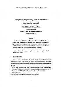
µ i (zi)
zi-
zi+
Figure 1. Objective function as a fuzzy number
4 Non-Fuzzy Multiobjective Problem A general linear multiple criteria decision making model can be presented as: Find a vector x written in the transformed form xT=[x1, x2,....,xn] which maximises objective functions n (4.1) max zi = å cij x j , j = 1,2 ,....n j =1 with constraints i=1,2,...,m, x ≥ 0 (4.2) åjaijxj ≤ bi where cij, aij and bi are crisp (non-fuzzy) values. This problem has been studied and solved by many authors. Zimmermann has solved this problem by using the fuzzy linear programming [21]. He formulated the fuzzy linear program by seperating every objective function zi, its maximum zi+ and minimum value zi- by solving (4.3) zi+ =max zi=åj cijxj and zi- = min zi=åj cijxj with constraints (2). Solutions zi+ and zi- are known as individual best and worst solutions respectively. Since for every objective function zi, its value changes linearly from zi- to zi+ it may be considered as a fuzzy number with the membership function µi(zi) as shown in Figure 1. ì0 ï ï (z −z − ) µ j( z j )= í i i ï ( zi + − zi − ) ï1 î
for zi ≤ zi − for zi − ≤ zi + , i = 1,2 ,....n
( 4.4 )
for zi ≥ zi +
According to Bellman-Zadeh 's principle of decision making in the fuzzy environment the grade of membership of a decision j, specified by objectives zj, is obtained by [1]. α = min µj(zj), j=1,2,..,k (4.5) or maxmin j subject to α ≤ µ j(zj), j =1,2,...,k and 0 ≤ α ≤ 1 (4.6)
According to this principle the optimal values of multicriteria optimisation correspond to maximum value of j. The auxiliary linear programme is obtained by: (4.7) z = maxα with constraints (6), taking into account (1) and (4) n ( zi − zi − ) − å cij x j + ( zi + − zi − )α ≤ i = 1,2 ,..., k ( zi + − zi − ) j =1
( 4.8 )
0 ≤ α ≤ 1, x j ≥ 0
j = 1,2 ,...., n
The original linear constraints (4.2) are added to these constraints. The problem can also be presented in a form (Lai and Hwang 1994): Find a vector x subject to
zi (x) ≥∼ zi0 ∀I x ε X
(4.9)
where zi , ∀i are corresponding goals, and ≥∼ is a soft or quasi inequality. The objective functions are assumed to be maximised max/min [ z1 (x)Ö . zi (x) ] (4.10) x ε X = {x|gs (x) {≥ = ≤}0, s=1,Ö ..,m} 0
where zj (x), jεJ are maximisation objectives, zi(x), iεI are the minimisation objectives, IUJ ={1,2,Ö , n} are considered as fuzzy constraints. All functions zj(x), gs(x) (i = 1,Ö ,n; s = 1,Ö ,m) can be linear and nonlinear. With the tolerances of fuzzy constraints given, the membership functions µi (x), ∀i could be established. The feasible set solution obtained through min-operator is defined by interaction of the fuzzy objective set. The feasible set is presented by its membership µD (x) = min (µi (x),Ö , µk (x),) If a decision maker deals with a maximum µD (x) in the feasible set then the solution procedure is max(miniµi (x),) x ε X. Suppose the overall satisfactory level of compromise is α = minµi (x) then the problem can be explained as Find max α subject to α≤µi (x) ∀i,
xεX
(4.11)
Assuming that membership functions, based on preference or satisfaction, are linear and non-decreasing between zi+ (x) and zi- (x) for ∀i ì1 if zi ( x ) f zi + ï ï ( z ( x ) − zi − ) if zi − ( x ) ≤ zi ( x ) ≤ zi + ( 4.12 ) µk ( x ) = í i + − ï ( zi − zi ) ï0 if zi ( x )p zi − î for ∀i.
The only feasible solution region is the area {x| zi -(x)≤ zi (x) ≤ zi+}∀i and xεX. Hence we can write Find max α subject to µk (x) =[ zi (x) - zi -] / [ zi+- zi -] ≥ α xεX
(4.13)
This problem can be solved by using two-phase approach. The first phase relates to the search for an optimal value of α0 in order to find a possible solution (x0). If the possible solution is unique, x0 is an optimal nondominated solution. Otherwise, the second phase is introduced to search for the maximum arithmetic mean value of all membership restricted by original constraints and αi≥α0∀i. That is Max (åi αi ) /i (4.14)
αí ≤ αi ≤ µi (x), ∀i, xεX for i objective functions and αí solution (4.7). The objective functions (4.10) could be written Max [åi µi (x)] /I (4.15) αí ≤ µi (x), ∀i, xεX by unifying both objectives (4.7) and (4.11) the second step can be automatically solved after the first step following the solution procedure of the simplex method: max α + δ[åi µi (x)] /I, α ≤ µi (x), ∀i, xεX (4.16) where δ is sufficiently small positive number. Since the weights between objectives are not equal we can write max α + δåiwi µi (x) α ≤ µi (x), ∀i, x ε X (4.17) for wi as the relative importance of the ith objective and åi µi = 1.The coefficient α represents the degree of acceptability or degree of possibility for the optimal solution. For construction industry activities18 the minimal value of the coefficient α1 and the maximal value of the coefficient αn can be prescribed. Hence two new constraints are added in this linear programme: α ≥ α1 α≤ αn (4.18) where 0 ≤ α ≤1 0 ≤ α, Coefficients of satisfaction (ϕI) in relation to the best individual solutions zi+ are ϕi = max zi/ zi+ i=1,2,....,n. (4.19) Lai and Hwang consider the equation (4.17) as an augmented max-min approach that is an extension of Zimmermannís approach. From the aspect of fuzzy set theory the augmented max-min approach allows for compensation among objectives. Firstly one reaches the solutions at a large unit, and then by reevaluating these solutions the compromise solutions at a smaller unit are obtained.
5 Fuzzy Multiobjective Problem The Fuzzy Multiple Objective Decision Model (FMODM) studied by Lai and Hwang [10] [12] states that the effectiveness of a decision makersí performance in
a decision process can be improved as a result of the high quality of analytic information supplied by a computer. They propose an Interactive Fuzzy Multiple Objective Decision Model (IFMODM) to solve a specific domain of Multiple Objective Decision Model (MODM). Max (zi(x)Ö ., zn(x) ) (5.1) subject to gj (x) ≤ ∼bj j=1,Ö ,m x≥0 where bj, ∀j are fuzzy resources available with corresponding maximal tolerances ti. Their membership functions are assumed to be non-increasing linear functions between bj and bj + tj. The objective functions (5.1) are redefined into Max zi(Ci, x) i=1,2Ö ,I (5.2) subject to
gj (A, x) {≤=≥} bj j=1,2,Ö ..m, x ≥ 0 Lai and Hwang [11] suggest presenting the model (5.2) limitations as fuzzy inequalities since the limitations prevent the objective functions from reaching their individual optimum. The solution of the model can be obtained by solving the following auxiliary problem: Find x, subject to gj(Aj,x)≤ bj, ∀j x≥0 (5.3) zi(Ci, x) ≥∼zi0 , ∀i where zi0 ,∀i are the goals of the objectives, and ≥∼ is a soft or fuzzy inequality. With the known tolerances of fuzzy constraints the membership functions µi (zi), ∀i to measure satisfaction levels of fuzzy objective constraints could be established. It is supposed that membership functions are based on a preference concept. The membership functions can be any non-decreasing functions for maximisation objectives and non-increasing functions for maximisation objectives such as linear, exponential, and hyperbolic. Lai and Hwang assume linear membership functions since the other types of membership functions can be transferred into equivalent linear forms [11]. Each objective of equation (5.2) should have an individual best (zi +) and individual worst solution (zi -) zi += max zi(Ci, x), x ε X zi -= min zi(Ci, x), x ε X (5.4) The linear membership function can be defined as in (4.8). According to (4.18) and (4.19) the following augmented problem can be defined
max α + δåiwi µi (x) α ≤ µi (x), ∀i, x ε X, αε [0,1]
(5.5)
where δ is a sufficiently small positive number, and wi (åiwi =1) is of relative importance or weight. If a decision maker wants to provide his/her goals zi0 and corresponding tolerances ti for objectives, than for zi0 ≤ zi + and (zi0 - tk)b ≥ zi - the problem will become:
Find x, subject to zi (Ci ,x) )≥∼zi0, ∀i
and x ε X
(5.6)
where zi ,∀i as well as their tolerances ti are given. Then max α + δåiwi µi (zi) 0
µ (zi) = 1 - [ zi0 ñ zi (Ci ,x) ]/ ti ≥ α xεX, αε[0,1]
(5.7)
The problem can be further considered as max α + δ[åi wiµi (zi) + δåjqjµj (gj) ]
(5.8)
subject to µi (zi) = [ zi (Ci ,x) ñ zi- ]/ [ zi+ - zi- ] ≥ α ∀I µj (gj) = 1- [ gj(Aj,x)- bj ] / tj ≥ α ∀j x>0, αε[0,1] where wi and gj , ∀i, j are of relative importance and åi wi + åj gj =1 According to this procedure the computer programme has been written in FORTRAN 77 programming language. Input data are: number of objectives k, number of constraints m, number of unknowns n, goals zi (i=1,2,..,k), elements cij (i=1,2,..,k; j=1,2,...,n),aij (i=1,2,..,n), bi (i=1,2,..,m), tolerances ti (i=1,2...,k) and di (i=1,2,...,m). The programme determines the individual best zi+ solution and the individual worst solution zi- for every objective i (i=1,2,...,k). The objective functions are (4.3) and the constraints are (4.2). The obtained values zj+ and zj-, based on the modified Zimmermann's procedure, are used to solve the linear programme with the objective function (4.17) and constraints (4.2), (4.8) and (4.18). For the nonfuzzy problem, this programme gives the values of unknown xj (j=1,2,..,n), maximal values of objective function zi (i=1,2,...,k), coefficient of acceptability α and coefficients of satisfaction ϕi (i=1,2,..,k). For the fuzzy problem, the linear programme with the objective function (5.3) and the constraints (5.6) gives: the optimal value of unknown xi (i=1,2,...,n), objective function zi , coefficients of satisfaction ϕi (i=1,2,..,k) and coefficient of acceptability α..
6 Case Study Analysis and Modelling The operations of a concrete manufacturing plant, which produces and transports concrete to building sites, have been analysed. Fresh concrete is produced at a central concrete plant and transported by seven transit mixers over the distance ranging 1500-3000 m (depending on the location of the construction site) to the three construction sites. Three concrete pumps and eleven interior vibrators are used for delivering, placing and consolidating the concrete at each construction site. Table 1 illustrates the manufacturing capacities of the plant, operational capacity of the concrete mixer, interior vibrator, pumps and manpower requirement at the three construction sites. A quick analysis will reveal the complexity of the variables and constraints of this concrete production plant and delivery system. The plant manager's task will be to optimise the profit by
utilizing the maximum plant capacity while meeting the three-construction site's concrete and other resource requirement through a feasible schedule. Table 1: Concrete plant capacity and construction site's resource demands Plant capacity Transit mixers (total = 7) Concrete pumps (total = 3) Interior vibrators (total = 11) Worker requirement Minimal concrete requirement (tolerance)
Concrete Plant 60 m3/h 2520m3 (weekly)
-
Site A
Site B
Site C
Remarks 200 m3 (tolerance)
- 8.45 m3/h
9.26 m3/h
7.26 m3/h
16 m3/h
22 m3/h
26 m3/h
operated by 7 workers operated by 6 workers
4.0 m3/h 5
6
7
9
14.0 m3/h 588 m3/week (47 m3)
18.0 m3/h 756 m3/week (60 m3)
21.5 m3/h 903 m3/week (72m3)
Weekly values are based on 42 working hours/week
6.1 Objective Formulation Success of any decision model will directly depend on the formulation of the objective function taking into account all the influential factors. We modelled the final objective function taking into account three independent factors: (1) profit expressed as $/m3 (2) index of work quality(performance) and (3) worker satisfaction Profit: The expected profit as related to the volume of concrete to be manufactured is modelled as the first objective and is shown in Table The minimal expected weekly profit as a fuzzy value is z0= AU$27,000 per week with tolerance, t1=AU$2,100. Table 2: Modelling profit as an objective
Site A
Site B
Site C
Expected profit (AU$/m3)
12
10
11
Index of quality: Equally or sometimes more important than the profit, quality plays an important role in every industry. We modelled the index of quality at construction sites, as the second objective. The index is ranged from 5 points/m3 (bad) quality to 10 points/m3 (excellent) quality and the assigned values are shown in Table 3. The minimal expected total weekly number of points for quality, as fuzzy value, is z02=21400 with tolerance, t2= 1700 points. Table 3: Modelling index of quality as an objective
Site A
Site B
Site C
Index of Quality
9
10
7.5
Worker Satisfaction Index: We modelled the index of worker satisfaction as the third objective and is ranged from 5 to 10 points per m3 of produced, transported and placed concrete. The assigned values are depicted in Table 4. The minimal expected total weekly number of points as a fuzzy value is z0=18000 with tolerance, t3=1400. Table 4: Modelling worker satisfaction index as an objective Worker Satisfaction Index
Site A 9
Site B
Site C
10
7.5
6.2 Variables that Optimise the Objective Function After knowing the objective function our next task is to determine the variables that optimises the objective function. In our problem it is to find: the optimal value of unknowns xi (i=1,2,3) that represent quantities of concrete which have to be delivered to Site A, B and C respectively and corresponding optimal values of the objective functions z1, z2, z3.. According to problem requirements and available data (Table 1,2,3 and 4) the objective functions can be modelled as follows [21]: ●
max z1=12x1+10x2+11x3 (>,∼) 27000 with tolerance, t1=2100 (profit)
●
max z2=9x1+10x2+ 7.5x3 (>,∼) 21400 with tolerance, t2=1700 (index of quality)
●
max z3= 8x1+7x2+9x3 (>,∼) 18000 with tolerance, t3=1400.(worker satisfaction index)
●
x1+x2+x3 (