Jul 13, 2012 - hydrogen atom and present results for excitation and ionization probabilities .... the atomic energy levels and dipole transition matrix elements.
PHYSICAL REVIEW A 86, 013410 (2012)
Application of a numerical-basis-state method to strong-field excitation and ionization of hydrogen atoms Shaohao Chen,1,* Xiang Gao,2 Jiaming Li,3,4 Andreas Becker,1 and Agnieszka Jaro´n-Becker1 1
Department of Physics, JILA, University of Colorado, Boulder, Colorado 80309-0440, USA 2 Beijing Computational Science Research Center, Beijing 100084, China 3 Department of Physics, Key Laboratory for Laser Plasmas (Ministry of Education), Shanghai Jiao Tong University, Shanghai 200240, China 4 Department of Physics, Center of Atomic and Molecular Nanosciences, Tsinghua University, Beijing 100084, China (Received 13 March 2012; published 13 July 2012) We apply a numerical-basis-state method to study dynamical processes in the interaction of atoms with strong laser pulses. The method is based on the numerical representation of finite-space energy eigenstates of the field-free atomic Hamiltonian in a box on a grid and the expansion of the solution of the full time-dependent Schr¨odinger equation, including the interaction with the field, in this numerical basis. We apply the method to the hydrogen atom and present results for excitation and ionization probabilities as well as photoelectron momentum distributions. Convergence of the results with respect to the size of the basis as well as the parallel efficiency of the numerical algorithm is studied. The results of the numerical-basis-state method are in good agreement with those of two-dimensional numerical grid calculations. The computation times for the numerical-basis-state method usually are found to be significantly smaller than those for the two-dimensional grid calculations, whereas, even higher excited states can be well represented. We further apply this method to study a few recently reported phenomena related to strong-field excitation of atoms, such as the dependence of the excitation probabilities on the carrier-envelope phase in ultrashort pulses as well as the so-called frustrated ionization. DOI: 10.1103/PhysRevA.86.013410
PACS number(s): 32.80.Rm, 32.80.Wr, 31.15.A−
I. INTRODUCTION
The progress in the development of intense laser systems is one of the reasons for the continuous research of the response of matter to an external electromagnetic field. Many novel aspects of light-matter interaction at the atomic and molecular levels have been discovered over the last few decades, e.g., above-threshold ionization [1], higher-order harmonic generation [2], or laser-induced tunneling [3,4]. Recent advances in laser technology extended the wavelength regime for ultrashort intense pulse generation significantly, which now spans from the extreme ultraviolet to the mid-infrared. At the same time, pulse durations decreased below the femtosecond (1 fs = 1 × 10⁻¹⁵ s) barrier. Ionization and excitation are an essential part of many laser-induced phenomena, including the recent observations of highly excited states by frustrated tunneling ionization [5], the enhanced emission of low-energy electrons at mid-infrared laser wavelengths [6], oscillatory patterns in the near-threshold electron angular distributions [7,8], multiple ionization events within one half-cycle of the laser electric field [9], or time-resolved holography [10]. In view of these activities, the development and application of different complementary theoretical methods for the analysis of laser-driven nonlinear processes in atoms and molecules is of great interest. Current approaches include, among others, approximative but powerful multiphoton and tunneling ionization formulas [11–14], nonperturbative Floquet methods [15,16], the time-dependent Hartree-Fock method [17], semiclassical approximation methods [18], classical-trajectory Monte Carlo simulations [19,20], as well as ab initio numerical methods to solve the time-dependent
*
Present address: Department of Physics and Astronomy, Louisiana State University, Baton Rouge, Louisiana 70803. 1050-2947/2012/86(1)/013410(9)
Schr¨odinger equation (TDSE) either on a large space-time grid [21–23] or via expansion into basis sets [24,25]. Solutions based on analytical-basis sets, e.g., Slater-type orbitals [26], Gaussian orbitals [27], or B splines [28], have a long tradition in atomic and molecular physics as well as chemistry. In electronic structure and materials calculations, there has been a recent upsurge in using numerical-basis sets [29,30] as an alternative to analytical-basis sets. Systematic studies concerning a comparison of the methods are rather scarce. However, it appears that calculations using numerical-basis sets may offer some advantages, e.g., in terms of computation efficiency, over analytical-basis sets (in particular, Gaussianbasis sets) in obtaining the geometries and binding energies of large molecular systems [31,32]. In view of this development, the question arises if a numerical-basis-state method can be applied with sufficient accuracy and reasonable computational effort to dynamical processes in a strong field, such as laserinduced excitation and ionization of atoms or molecules. In this article, we investigate the feasibility of using numerical-basis states to solve the time-dependent Schr¨odinger equation in strong-field physics problems. To this end, we numerically obtain finite-space energy eigenstates for the hydrogen atom in a box [33,34], represent the numericalbasis set on a grid, and propagate the system under the influence of an intense laser pulse. As examples, we calculate the transition probabilities to excited bound states and into the continuum as well as electron momentum spectra. In order to test the method, laser parameters, such as wavelength, intensity, pulse length, and carrier-envelope phase (CEP) are varied. The results of the numerical-basis-state method are in good agreement with results obtained by propagating the wave function on a space-time grid. The rest of the paper is organized as follows. In Sec. II, we introduce the numerical-basis-state method as well as the
013410-1
©2012 American Physical Society
´ CHEN, GAO, LI, BECKER, AND JARON-BECKER
PHYSICAL REVIEW A 86, 013410 (2012)
numerical techniques used to propagate the wave function and to obtain excitation and ionization probabilities as well as momentum spectra. Next, in Sec. III, we discuss some aspects of the implementation, such as the basis size as well as the efficiency of a parallelization of the computer code. We further present comparisons of the results obtained with the numerical-basis-state method with those from space-time grid calculations. The numerical-basis-state method is then applied to an analysis of different phenomena related to the excitation of an atom in short intense laser pulses in Sec. IV. The paper ends with a summary. II. SOLUTION OF TDSE USING NUMERICAL-BASIS STATES
In this section, we first obtain finite-space energy eigenstates for the hydrogen atom in a box by solving the eigenvalue problem of the field-free atomic Hamiltonian. To solve the TDSE for the atom interacting with a laser pulse, we represent the basis states on a grid and expand the full solution of the TDSE in the basis. The propagation of the solution under the influence of a short laser pulse requires the solution of a set of linear equations for the expansion coefficients, which gives us direct access to certain observables as well. We have chosen to study the interaction of the hydrogen atom with the field since a comparison with ab initio space-time grid calculations can be performed without approximating electron correlation effects via an effective potential. It is, however, straightforward to extend the numerical-basis method to other atoms within the single-active electron approximation. A. Numerical-basis states
Functions of numerical-basis sets are written, as in the case of analytical-basis sets, as products of a radial wave function and the appropriate spherical harmonic ψn,l,m (r) = Rnl (r)Ylm (�). The radial functions are generated as solutions of the radial Schr¨odinger equation (Hartree atomic units e =m=h ¯ = 1 are used unless mentioned otherwise), � � 1 d2 1 − + V − (r,l) unl (r) = Enl unl (r), (1) eff 2 dr 2 r where unl (r) = rRnl (r) and Veff (r,l) = l(l + 1)/(2r 2 ) is an effective potential corresponding to the orbital angular momentum quantum number l. The eigenvalue equation (1) is solved on a one-dimensional finite-space grid with a boundary condition, using the Numerov method. In principle, any boundary condition could be adopted here. We use the most common one, namely, unl (0) = unl (R0 ) = 0,
(2)
where R0 is the outer boundary of the grid. Usually, R0 is chosen to be large enough such that the numerical solutions for a significant number of bound states agree (within numerical errors) with the exact analytical solutions, in case the latter are available. Therefore, the energetically lowest n0 eigenstates in the numerical-basis set can be considered as (numerically) exact eigenstates of the system. On the other hand, the boundary condition (2) leads to a selection of those continuum states of the original problem,
which have a node at R0 , and, hence, to a discretization of the continuum [35]. The density of states in the discretized continuum is determined via the extension of the grid R0 . The number of states in the continuum is, in practice, limited by the grid separation, which effectively determines the largest frequency of the oscillating continuum states. Due to the discretization, the continuum states can also be indexed by the discrete principal quantum numbers n. The number of nodes of bound and continuum states is given by n − l − 1, and all states are orthogonalized using the Gram-Schmidt method. Thus, in general, the bound and continuum states form a complete basis set. In the course of computations, the number of continuum states is usually further limited by practical reasons and/or the concrete problem. The discretization of the continuum via a boundary condition is widely used in the solution of the TDSE with analytical-basis sets as well, e.g., using B splines [28]. In contrast to the analytical-basis-state methods, we do not proceed by approximating the numerical solution (often, in a subspace) by analytical functions but use the numerical values on the radial grid points directly. To this end, the grid points can be equally distributed, or a higher concentration of grid points near the nucleus can be used. We have used a square grid with a higher concentration of grid points near the nucleus, i.e., ri = i 2 R0 /N 2 . Furthermore, in the present application of the method, the outer boundary (R0 ) and the total number of grid points (N ) are chosen to be adaptive for different n and l. Larger R0 and N are chosen for larger n and l. This kind of numerical-basis set has been used before to calculate atomic photoabsorption spectra for highly excited states as well as continuum states [33,34]. These previous results indicate that the atomic energy levels and dipole transition matrix elements can be well reproduced using the numerical-basis set. B. Propagation of the wave function
In order to solve the TDSE for the hydrogen atom interacting with an intense laser pulse, we use a standard technique. The three-dimensional TDSE is given by ∂�(r,t) = H (r,t)�(r,t), ∂t
(3)
1 1 H (r,t) = − ∇ 2 − − E(t) · r, 2 r
(4)
i with
as the Hamiltonian in dipole approximation using a length gauge. The time-dependent wave packet is then expanded in the finite-space energy eigenstates as � �(r,t) = cnlm (t)ψnlm (r). (5) n,l,m
Substituting Eq. (5) into Eq. (3), one obtains the TDSE in a vector-matrix form i
∂C(t) = H(t)C(t), ∂t
(6)
where the elements of vector C(t) are expansion coefficients cnlm (t) and the elements of Hamiltonian matrix H(t) are
013410-2
APPLICATION OF A NUMERICAL-BASIS-STATE METHOD . . .
given by hn� l � m� ,nlm (t) =
�
ψn∗� l � m� (r)H (r,t)ψnlm (r)d r.
(7)
The Hamiltonian matrix is block tridiagonal due to the dipole selection rule for the angular momentum (l � = l ± 1). Integrating the TDSE (6) and calculating the propagator using the Crank-Nicolson approximation, we obtain a set of linear equations, � � �� �t �t I+i H t + C(t + �t) 2 2 �� � � �t �t C(t), (8) = I−i H t + 2 2 where �t is the time step of propagation. The formalism up to now holds for any kind of polarization of the electric field (i.e., linear, circular, or elliptical). Specifically, for linear polarization in the z direction, the electric field of a laser pulse can be written as � � 2 πt sin(ωt + φ), (9) E(t) = E0 sin T0 where E0 is the field strength, T0 is the time duration of the pulse, ω is the field frequency, and φ is the CEP. Furthermore, in this case, the dipole selection rule m� = m restricts the basis set in m to those functions having the same azimuthal quantum number as the initial state (m = 0 for the ground state of the hydrogen atom). We will, therefore, drop the index m below. We solve the set of equations (8) using the portable extensible toolkit for scientific computation (PETSC) library [36], which is a widely used parallel code for solving linear systems based on Krylov subspace iteration methods [37]. It is known that the Krylov method provides high efficiency for problems with a sparse matrix as in our case. The parallel scheme we implemented is straightforward and is based on the message passing interface. The vector-matrix objects are distributed to different memories, and the vector-matrix options are parallel computed by different processors. In Sec. III B, we present results of tests concerning the parallel efficiency of the code. C. Observables
Observables, such as transition probabilities, energy, or momentum spectra, can be calculated based on the fieldfree-basis representation at the end of the laser pulse as well as at time instants when the laser electric field is zero. As mentioned above, the numerical-basis functions for the energetically lowest bound states represent the (numerically) exact solutions of the system. Therefore, the absolute square of the corresponding expansion coefficients |cnlm (ti )|2 directly represents the excitation probabilities for Enlm < 0, where ti is a time instant when the laser electric field is zero. Consequently, the total ionization probability is given by � |cnlm (ti )|2 . (10) Pion (ti ) = 1 − En,l,m 0) states as well as the total number of basis functions are determined by lmax , nmax , and R0 . For a grid size of R0 = 1000, bound states up to n = 20 are well represented on the grid. We have varied the basis size parameters up to lmax = 50 and nmax = 500, which results in a total number of numerical-basis set functions of up to about 24 200. In Table I, TABLE I. Absolute errors of some states (n,l) of the numericalbasis set with respect to the exact analytical energies En = −1/2n2 (second column) for the hydrogen atom. n
En
l=0
l=1
l=9
1 2 5 10 15 20
−5.00 × 10⁻¹ −1.25 × 10⁻¹ −2.00 × 10⁻² −5.00 × 10⁻³ −2.22 × 10⁻³ −1.25 × 10⁻³
+2.0 × 10⁻⁸ +2.0 × 10⁻⁸ +8.0 × 10⁻⁹ +2.3 × 10⁻⁹ +7.2 × 10⁻¹⁰ +3.8 × 10⁻⁸
+0.0 × 10⁻¹⁰ +5.0 × 10⁻⁹ +1.9 × 10⁻⁹ +6.2 × 10⁻¹⁰ +3.6 × 10⁻⁸
+0.0 × 10⁻¹⁰ +1.2 × 10⁻¹⁰ +4.2 × 10⁻⁹
013410-3
´ CHEN, GAO, LI, BECKER, AND JARON-BECKER 10 -5
6.2
(b)
6
5.8
5.8 P2
P2
6
5.6
5.6
5.8 5.6
5.4 5.2 20
25
30
2.4
35
5.8 5.6
5.4 40
45
5.2 400
50
lmax
10 -4
425
2.4
(c)
475
500
475
500
(d)
P4
2.3
2.2
2.2
2.1
2.1
2.24
20
25
2.22 30 35
40
45
2.24
400
50
425
lmax
1.7
-6
10 (e)
1.7 P20
10
P20
450
nmax
10 -4
2.3 P4
10 -5
6.2 (a)
PHYSICAL REVIEW A 86, 013410 (2012)
1.6 2
1.5 20
25
30
0 35 lmax
45
50
nmax
-6
(f)
1.6 2
1.5 40
2.22 450
400
425
0 450
nmax
475
500
FIG. 1. Squares: Excitation probabilities to the (a) and (b) second, (c) and (d) fourth, and (e) and (f) 20th excited states of a hydrogen atom in a two-cycle laser pulse at a wavelength of 800 nm, a peak intensity of 1 × 10¹⁴ W/cm2 , and a carrier-envelope phase of φ = 0. Panels on the left show the results as a function of lmax (with nmax = 500), and those on right show the results as a function of nmax (with lmax = 50). The convergence of the results is shown on a relative scale (main figure, ±10% of the respective final result) and on an absolute scale (insets, ±1% of the largest excitation probability).
we present the absolute error of the energies of some states of the numerical-basis set, calculated using the largest basis set, with respect to the analytical known energies for the hydrogen atom. An excellent agreement is found. In Fig. 1, we present probabilities for excitation of the hydrogen atom to the (a) and (b) second, (c) and (d) fourth, and (e) and (f) 20th excited states as functions of lmax (with nmax = 500, left column) and nmax (with lmax = 50, right column). The excitation probabilities for the nth state are summed up over l = 0 to l = n − 1. The results are shown on two scales, namely, within ±10% of the final result for the present excited state (main figure, relative error) and in the insets within ±1% of the largest excitation probability (i.e., P4 , ± 2.23 × 10⁻⁶ , absolute error). In the corresponding calculations, we considered a two-cycle pulse at 800 nm, a peak intensity of 1 × 10¹⁴ W/cm2 , and a carrier-envelope phase of φ = 0. The convergence of the results for the excitation probabilities is clearly seen. In particular, the convergence to a rather small absolute error shows the reliability of the method. As one would expect, the size of the basis with respect to lmax has to be larger for the higher excited states. In further test calculations, we have found that the trend shown in Fig. 1 holds for other field parameters as well. However, the relative and absolute errors increase with an increase in the wavelength, the peak intensity, and/or the pulse duration. These findings
FIG. 2. (Color online) (a) Speedup factor and (b) parallel efficiency as a function of the number of processors p. Laser parameters are the same as in Fig. 1. The red dashed line indicates the ideal linear speedup.
qualitatively agree with common expectations for these kinds of basis set calculations in which the basis size needs to be adjusted in view of the problem of interest. B. Parallel processing efficiency
As mentioned in Sec. III B, we implemented the numericalbasis-state method in a parallel processing code. In Fig. 2, we report test results of our investigations of the parallel efficiency. To this end, we determined the speedup factor, defined as Sp =
T1 , Tp
(13)
where T1 and Tp were the computational times with a single processor and p processors, respectively, and the parallel efficiency given by Ep =
Sp T1 = . p pTp
(14)
The actual speedup [Fig. 2(a)] is not far from the ideal linear case. Although the parallel efficiency [Fig. 2(b)] first slightly drops as the number of processors increases, it appears that the efficiency converges to about 80% for a larger number of processors used. In particular, the parallel efficiency Ep does not drop as 1/ ln(p) as in the case of algorithms, which are hard to parallelize. C. Comparison with results of grid calculations
In order to further test the numerical-basis-state method, we also numerically solved the TDSE for the hydrogen atom interacting with a linearly polarized laser pulse on a spatial grid directly. Due to rotational symmetry over the polarization axis (chosen here as the z axis), the Hamiltonian of the system in dipole approximation using a length gauge can be expressed
013410-4
APPLICATION OF A NUMERICAL-BASIS-STATE METHOD . . .
PHYSICAL REVIEW A 86, 013410 (2012)
TABLE II. Excited-state probabilities (multiplied by 10−4 ) as a function of principal quantum number n. An 800-nm laser pulse with a peak intensity of 1 × 10¹⁴ W/cm2 is used. Number of cycles (nc ) and CEP (φ) are nc = 2 and φ = π /2, respectively.
TABLE III. Excited-state probabilities (multiplied by 10−3 ) as a function of principal quantum number n. Laser parameters are the same as in Table II, except for nc = 10.
n
Basis-state method
Grid method
2 3 4 5 6 7 8 9 10
0.63 0.27 0.11 1.08 1.83 1.23 0.81 0.56 0.40
0.68 0.28 0.11 1.12 1.82 1.26 0.83 0.57 0.41
in cylindrical coordinates as H (ρ,z,t) =
pρ2 pz2 1 + − − zE(t), (15) 2 2 2 ρ + z2 + a 2
where z,ρ and pz ,pρ are the coordinates and corresponding momenta of the electron parallel and perpendicular to the polarization direction of the laser. a 2 = 0.001 is a soft-core Coulomb parameter, and E(t) is the electric field. The wave function of the initial (ground) state was obtained by imaginary time propagation without the field. We used the CrankNicolson method for the time propagation of a wave packet and a three-point differential formula to discretize the Laplacian on the spatial grid. Spatial steps of �ρ = �z = 0.1 a.u. and a time step of �t = 0.03 a.u. were used in the calculations. In order to represent well the spatial distributions of the excited-state wave functions up to n = 10, a grid with 2000 points in the ρ direction and 4000 points in the z direction was used for the wave-packet propagation in the presence of the laser field. Energies of the ground and excited states depend on the grid parameters as well as the soft-core parameter a. For the parameters in the present calculations, the relative errors of the energies with respect to the analytical results are up to 2 × 10⁻⁴ , and, hence, about 4 orders of magnitude larger than in the present numerical-basis-state approach. Mask functions were used at the boundary of the grid to absorb the outgoing wave packet. The excited-state probabilities (up to n = 10) are calculated by projecting the wave packet to field-free eigenstates at the end of the pulse. In Tables II and III, we compare the excitation probabilities calculated by the numerical-basis-state method and the spacetime grid method as a function of the principal quantum number n (summed over l = 0, . . . ,n − 1) for a two-cycle (Table II) and a ten-cycle (Table III) pulse at 800 nm, 1 × 10¹⁴ W/cm2 , and φ = π/2. For the shorter pulse length, the results agree well with each other, and the discrepancy is even well within the error margins found for the present basis set calculations (see Fig. 1). The results for the longer pulses show, however, that this difference between the numericalbasis state and the space-time grid results increases for longer pulses. As mentioned above, the relative errors for the excitedstate energies are considerably larger in the space-time grid method than for the numerical-basis-state method at present parameters. Consequently, transition amplitudes differ in the
n
Basis-state method
Grid method
2 3 4 5 6 7 8 9 10
0.023 0.118 0.490 1.741 0.126 0.043 0.042 0.049 0.036
0.026 0.131 0.423 1.900 0.197 0.024 0.009 0.012 0.019
two methods, and the differences between the final excitation probabilities increase with increases in the pulse length. By varying the grid and soft-core parameters, we have checked that the discrepancies in Table III can be well explained by the above-described inaccuracies in the two-dimensional (2D) grid method. Despite the discrepancies, the major features (e.g., maximum population at n = 5 and minor population for n > 6) are confirmed in both methods, whose physical mechanism is discussed in Sec. IV. Since the convergence of the results within the present numerical-basis-state method is demonstrated in Table I and Fig. 1, we refrained from further improving on the numerical error within the 2D grid method, which would result in a significant increase in computation time for a method outside the focus of the present paper. In general, we note that the computational effort to obtain accurate values for the probabilities in the highly excited states using the numerical-basis-state method is considerably less than that using the 2D grid method. This is partially due to the fact that the required number of numerical-basis-state functions (about 2.4 × 10⁴ in the present calculations) is much smaller than the required number of points (2000 × 4000 = 8 × 10⁶ ) in the present 2D grid calculations. Despite the fact that the total number of points in the 2D grid calculations is much larger than in the numerical-basis-state method, the 2D grid has smaller extensions (zmax = 200 vs R0 = 1000). Therefore, much higher excited states (up to n = 20, see Fig. 1) are well represented in the numerical-basis states. To cover the same number of excited states in the 2D grid calculations would require a large increase in the computational costs. Next, we consider ionization and the differential momentum distributions of the photoelectron. For this set of calculations, a larger numerical-basis set with lmax = 50 and nmax = 600 is used in order to cover the continuum states up to k = 1.5 a.u. In Fig. 3, we present the momentum distributions as a function the momentum components parallel (kz ) and perpendicular (kρ ) to the polarization direction of the linearly polarized field at 5 × 10¹³ W/cm2 (upper row) and 1 × 10¹⁴ W/cm2 (lower row) at 800 nm and φ = 0 in a six-cycle pulse. The results obtained with the numerical-basisstate method are shown on the left, whereas, the panels on the right present the 2D grid results. The results agree very well and show the expected ring structures, which correspond to the multiphoton
013410-5
´ CHEN, GAO, LI, BECKER, AND JARON-BECKER
PHYSICAL REVIEW A 86, 013410 (2012)
10 -4 4 P
n
(a)
2
P
n
0 2 10 -4 6
FIG. 3. (Color online) Comparison of differential momentum distributions of the photoelectron (on a logarithmic scale) induced by laser pulses (φ = 0) with 800 nm, six cycles, [(a) and (b)] 5 × 10¹³ W/cm2 and [(c) and (d)] 1 × 10¹⁴ W/cm2 , using left column: the basis-state method and right column: the 2D grid method.
10
12
14
(b)
4
6
8
10
12
14
P
n
(c)
1
0 2
4
6
8 n
10
12
14
FIG. 4. (Color online) Excited-state probabilities as a function of principal quantum number n. An 800-nm laser pulse with a peak intensity of 1 × 10¹⁴ W/cm2 is used. Number of cycles (nc ) and CEP (φ), respectively, are as follows: (a) nc = 2; (b) nc = 5; (c) nc = 10; black solid line with open circles: φ = 0; red dashed line with solid squares: φ = π/4; blue dashed-dotted line with hatched diamonds: φ = π/2.
(c)] pulse considered in the present calculations, there is a clear maximum at l = n − 1 = 4, indicating an even-number photon process (due to �l = ±1 for long pulses). At five
Pl
We have further applied the numerical-basis-state method to investigate several phenomena regarding the population in excited states recently reported in the literature. First, it has been found that, in ultrashort few-cycle laser pulses, the population in bound states does depend on the CEP of the pulse [41,42]. This effect is further investigated in the results shown in Fig. 4 where we present the excited-state probabilities as a function of the principal quantum number n (summed over l = 0, . . . ,n − 1) for laser pulses with (a) two, (b) five, and (c) ten cycles at 800 nm and 1 × 10¹⁴ W/cm2 and different carrier-envelope phases (open circles: φ = 0, solid squares: φ = π/4, and hatched diamonds: φ = π/2). The number of cycles (nc ) accounts for the full duration of the laser pulse. For the ten-cycle pulse, the distribution is strongly peaked with the maximum at n = 5 independent of the value of the CEP, which is probably due to multiphoton resonant absorption. However, at shorter pulses, the distribution smears out more and more, and maxima at different n appear, which clearly shows the strong dependence of the excited-state population on the CEP of the few-cycle pulse. We have further computed the corresponding distributions over the angular quantum number l for the n = 5 state at 800 nm, 1 × 10¹⁴ W/cm2 , and φ = π/4. The results in Fig. 5 show strong dependence of the distribution on the number of cycles in the pulses. For the longest [ten-cycle, panel
8
4
0 2 10 -3 2
Pl
IV. EXCITED-STATE POPULATION IN ULTRASHORT LASER PULSES
6
2
Pl
above-threshold ionization process. Both results also show the typical radial fanlike pattern and the node structure in the angular distribution, which has been observed in experiments [7,38] and previous theoretical papers [8,39]. Results of the test calculations indicate that, for the current basis-state and grid parameters, the small differences in the distributions at larger momenta are caused by the 2D grid calculations. Similar agreement between the results of the two methods has been found at other laser parameters, for example, the asymmetry in the photoelectron momentum distributions in few-cycle pulses as a function of the carrier-envelope phase could be well reproduced (e.g., Ref. [40]).
4
1.5 1 0.5 0 2.5 2 1.5 1 0.5 0 1.5 1 0.5 0
10 -4 (a)
0 10
1
2
3
4
1
2
3
4
1
2 l
3
4
-4
(b)
0 10
-3
(c)
0
FIG. 5. Excited probabilities as a function of angular quantum number l in the n = 5 state. An 800-nm laser pulse with a peak intensity of 1 × 10¹⁴ W/cm2 and φ = π/4 is used. Number of cycles: (a) nc = 2, (b) nc = 5, and (c) nc = 10.
013410-6
0.03 0.025 0.02 0.015 0.01 0.005 0
0.01 0.008 0.006 0.004 0.002 0
0
0
1
1
2
2
3
3
4
4
1 2 3 4 Number of cycles
Five cycles
Ten cycles
5
5
5
1 0.99 0.98 0.97 0.96
0.03 0.025 0.02 0.015 0.01 0.005 0
0.03 0.025 0.02 0.015 0.01 0.005 0
0
2
4
6
8
10
P5
Excitation probability
0
PHYSICAL REVIEW A 86, 013410 (2012)
P2
Five cycles 1 0.995 0.99 0.985 0.98 0.975
Ionization probability
Ground-state probabilities
APPLICATION OF A NUMERICAL-BASIS-STATE METHOD . . .
0
2
4
6
8
10
0.02 0.015 0.01 0.005 0
0.0005 0.0004 0.0003 0.0002 0.0001 0
0
0
1
2
3
4
1 2 3 4 Number of cycles
Ten cycles
5
5
0.02 0.015 0.01 0.005 0 0.002 0.0015 0.001 0.0005 0
0
2
4
0
2 4 8 10 6 Number of cycles
6
8
10
FIG. 7. Time-dependent excitation probabilities in upper row: n = 2 and lower row: n = 5. An 800-nm laser pulse with a peak intensity of 1 × 10¹⁴ W/cm2 and φ = π/2 is used. Number of cycles: left: nc = 5; right: nc = 10. 0
2 4 8 10 6 Number of cycles
FIG. 6. Time-dependent excitation and ionization probabilities. An 800-nm laser pulse with a peak intensity of 1 × 10¹⁴ W/cm2 and φ = π/2 is used. Number of cycles: left: nc = 5; right: nc = 10. First row: n = 1, second row: total excitation, and third row: total ionization.
cycles [panel (b)], the population is more broadly distributed, however, the probabilities in the even-l states (l = 0,2,4) are clearly larger than those in the odd-l states (l = 1,3), which is still in agreement with the conclusion of an even-number photon resonant absorption for the n = 5 state. For the shortest pulse, the population is distributed at the largest even- as well as odd-l values, indicating that the resonant character of the transition is lost. The expansion in numerical-basis states also provides access to the probabilities in the bound and continuum states during the interaction whenever the electric field is zero. This gives further information into the excitation and ionization dynamics during the pulse. In Fig. 6, we present the probabilities to find the hydrogen atom in its ground state (upper row), in the excited bound states (second row), and in the continuum states (lower row) as a function of time for five- (left-hand side) and ten-cycle (right-hand side) pulses at 800 nm, 1 × 10¹⁴ W/cm2 , and φ = π/2. We observe that the total excitation probability is built up over the raise of the pulse and is largest at the peak of the pulse, whereas, in the back of the pulse, this population is partially transferred back to the ground state. The ionization probability increases, as one would expect, during the front part of the pulse up to the peak, after which, it remains almost constant. Further analysis (Fig. 7) indicates that, during the front part of the pulse, mainly the lowest excited states (in particular, n = 2) are strongly populated, whereas, the population in the higher excited states (e.g., n = 5) increases during the interaction at the back part of the pulse. In order to further investigate the excitation and ionization dynamics, we performed another set of calculations in which we shaped either the front or the back part of the pulse. To this
end, we considered the following laser electric fields:
2k � πt sin T0 : 0 � t � T20 , � T0 Ek,j (t) = E0 sin(ωt + φ) sin2j πt : 2 < t � T0 , T0
(16)
where an increase in the parameter k (j ) indicates an increasingly steepened front (back) edge of the pulse. The corresponding results in Fig. 8 show that the excitation probability for the sin2 pulse and the steepened front-shaped pulse virtually agree over the back part of the pulse, which is in agreement with dominant resonant multiphoton transitions at rather weak electric fields. On the other hand, for the pulse with a steep back part, the final excitation probability is slightly larger since the
FIG. 8. (Color online) (a) Ground state, (b) excitation, and (c) ionization probability as a function of time. Black solid line: sin2 -shaped pulse; red dashed line: front-shaped pulse (k = 8, j = 1); blue dotted line: back-shaped pulse (k = 1, j = 8). The number of cycles was nc = 20, whereas, other laser parameters are the same as in Fig. 4.
013410-7
´ CHEN, GAO, LI, BECKER, AND JARON-BECKER 10
PHYSICAL REVIEW A 86, 013410 (2012)
population of the states with n � 7 for the longer pulse length in agreement with the expectation for a frustrated ionization effect. These results are also in qualitative agreement with the first experimental observations of the effect for the helium atom [5]. In contrast, the maximum in the excited-state population at n = 5 occurs independent of the length of the pulse (see also, Fig. 4) and is likely due to a resonance phenomenon.
−3
2
Pn
(a)
1
0
5
10
10
15
20
V. SUMMARY
n
−4
6 (b)
Pn
4 2 0
5
10
15
20
n
FIG. 9. Excited-state probabilities as a function of principal quantum number n for interaction of the hydrogen atom with an 800-nm laser pulse with a peak intensity of 1 × 10¹⁴ W/cm2 and (a) 10 cycles and (b) 20 cycles of field oscillation.
population transfer from the lowest excited states to the ground state is strongly altered. The final ionization probabilities due to the interaction with the shaped pulses are smaller than for the sin2 pulse but do agree well with each other. This supports the interpretation that the final ionization probability strongly depends on transition into the continuum at the largest field strength near the peak of the pulse. Finally, we studied the population in highly excited bound states with respect to the recently reported phenomenon called frustrated ionization [5]. It specifies the experimental observation that, in a laser field at laser intensities well in the so-called tunneling regime, the electron may be left in highly excited states. This observation has been explained by a deacceleration of the electron over many laser cycles and a recapturing of the electron once the laser pulse ceases. While frustrated ionization has first been observed for a single ionization of atoms [5], similar effects have recently been reported for the dissociation of molecules [43–45] and the nonsequential double ionization of atoms [46]. According to the present interpretation of the effect, the population in the highly excited states should occur in long pulses only. We have, therefore, performed simulations using the numerical-basis-state method for the interaction of a hydrogen atom with laser pulses of 10 and 20 cycles at an intensity of 1 × 10¹⁴ W/cm2 and a wavelength of 800 nm. The results, presented in Fig. 9, clearly show a much stronger
[1] P. Agostini, F. Fabre, G. Mainfray, G. Petite, and N. K. Rahman, Phys. Rev. Lett. 42, 1127 (1979). [2] A. McPherson, G. Gibson, H. Jara, U. Johann, T. S. Luk, I. A. McIntyre, K. Boyer, and C. K. Rhodes, J. Opt. Soc. Am. B 4, 595 (1987).
We have developed a numerical-basis-state method for the interaction of single-active electron systems with intense laser pulses. The method is based on the representation of numerical solutions of the unperturbed system on a grid, which, in the case of an atomic system, can be chosen to be one dimensional along the radial direction. The solutions form a numerical-basis set of bound and continuum states of the system. For the interaction with the external field, the time-dependent solution of the corresponding Schr¨odinger equation is expanded in the numerical-basis set, and the expansion coefficients are obtained via a set of linear equations during the propagation. We have applied the method to the interaction of the hydrogen atom with short intense laser pulses and have obtained excitation and ionization probabilities as well as momentum distributions of the photoelectron. Convergence of the results as a function of the size of the basis set as well as results for the parallel processing efficiency of the numerical algorithm have been presented. We have further shown that the results of the numerical-state method are in good agreement with those obtained in two-dimensional grid calculations. The comparison shows that computation times within the numerical-basis-state method are often favorable as compared to two-dimensional grid calculations. Furthermore, in the numerical-basis-state method, it is possible to study excitation for highly excited states, which is often associated with high computational costs in a 2D grid calculation. Finally, we have shown that phenomena, which have recently been reported in the literature, can be well reproduced with the present numerical-basis-state method. This includes the dependence of the excitation probability in low-lying states on the carrier-envelope phase in ultrashort laser pulses as well as the phenomenon of frustrated ionization with strong population of highly excited states in longer pulses. ACKNOWLEDGMENTS
We acknowledge financial support through the AFOSR MURI “Mathematical Modeling and Experimental Validation of Ultrafast Light-Matter Coupling associated with Filamentation in Transparent Media,” Grant No. FA9550-10-1-0561.
[3] J. E. Decker, G. Xu, and S. L. Chin, J. Phys. B 24, L281 (1991). [4] F. A. Ilkov, J. E. Decker, and S. L. Chin, J. Phys. B 25, 4005 (1992). [5] T. Nubbemeyer, K. Gorling, A. Saenz, U. Eichmann, and W. Sandner, Phys. Rev. Lett. 101, 233001 (2008).
013410-8
APPLICATION OF A NUMERICAL-BASIS-STATE METHOD . . .
PHYSICAL REVIEW A 86, 013410 (2012)
[6] C. I. Blaga, F. Catoire, P. Colosimo, G. G. Paulus, H. G. Muller, P. Agostini, and L. F. DiMauro, Nat. Phys. 5, 335 (2009). [7] A. Rudenko, K. Zrost, C. D. Schr¨oter, V. L. B. de Jesus, B. Feuerstein, R. Moshammer, and J. Ullrich, J. Phys. B 37, L407 (2004). [8] D. G. Arb´o, S. Yoshida, E. Persson, K. I. Dimitriou, and J. Burgd¨orfer, Phys. Rev. Lett. 96, 143003 (2006). [9] N. Takemoto and A. Becker, Phys. Rev. Lett. 105, 203004 (2010). [10] Y. Huismans, A. Rouz´ee, A. Gijsbertsen, J. H. Jungmann, A. S. Smolkowska, P. S. W. M. Logman, F. L´epine, C. Cauchy, S. Zamith, T. Marchenko, J. M. Bakker, G. Berden, B. Redlich, A. F. G. van der Meer, H. G. Muller, W. Vermin, K. J. Schafer, M. Spanner, M. Yu. Ivanov, P. Smirnova, D. Bauer, S. V. Propruzhenko, and M. J. J. Vrakking, Science 331, 61 (2011). [11] L. V. Keldysh, Zh. Eksp. Teor. Fiz. 47, 1945 (1964) [Sov. Phys. JETP 20, 1307 (1965)]. [12] A. M. Perelomov, V. S. Popov, and M. V. Terent’ev, Sov. Phys. JETP 23, 924 (1966). [13] F. H. M. Faisal, J. Phys. B 6, L89 (1973). [14] H. R. Reiss, Phys. Rev. A 22, 1786 (1980). [15] S.-I. Chu and J. Cooper, Phys. Rev. A 32, 2769 (1985). [16] P. G. Burke, P. Francken, and C. J. Joachain, J. Phys. B 24, 761 (1991). [17] K. C. Kulander, Phys. Rev. A 36, 2726 (1987). [18] G. van de Sand and J. M. Rost, Phys. Rev. A 62, 053403 (2000). [19] C. R. Feeler and R. E. Olson, J. Phys. B 33, 1997 (2000). [20] J. S. Cohen, Phys. Rev. A 64, 043412 (2001). [21] K. C. Kulander, Phys. Rev. A 35, 445 (1987). [22] K. J. Schafer and K. C. Kulander, Phys. Rev. A 42, 5794 (1990). [23] J. S Parker, B. J. S. Doherty, K. J. Meharg, and K. T. Taylor, J. Phys. B 36, L393 (2003). [24] E. Cormier and P. Lambropoulos, J. Phys. B 30, 77 (1997). [25] S. Dionissopoulou, T. Mercouris, A. Lyras, and C. A. Nicolaides, Phys. Rev. A 55, 4397 (1997).
[26] E. Clementi and C. Roetti, At. Data Nucl. Data Tables 14, 177 (1974). [27] A. Szabo and N. S. Ostlund, Modern Quantum Chemistry (Dover, New York, 1996). [28] H. Bachau, E. Cormier, P. Decleva, J. E. Hansen, and F. Mart´ın, Rep. Prog. Phys. 64, 1815 (2001). [29] B. Delley, J. Chem. Phys. 92, 508 (1990). [30] B. Delley, J. Chem. Phys. 113, 7756 (2000). [31] N. A. Benedek, I. K. Snook, K. Latham, and I. Yarovsky, J. Chem. Phys. 122, 144102 (2005). [32] D. J. Henry, A. Varano, and I. Yarovsky, J. Phys. Chem. A 112, 9835 (2008). [33] Chen Shaohao and Li Jiaming, Chin. Phys. Lett. 23, 2717 (2006). [34] Gao Xiang, Chen Shaohao, and Li Jiaming, Chin. Phys. Lett. 26, 013102 (2009). [35] B. W. Shore, J. Phys. B 7, 2502 (1974). [36] http://www.mcs.anl.gov/petsc/petsc-as/index.html. [37] P. N. Brown and Y. Saad, SIAM J. Sci. Stat. Comput. 11, 450 (1990). [38] C. M. Maharjan, A. S. Alnaser, I. Litvinyuk, P. Ranitovic, and C. L. Cocke, J. Phys. B 39, 1955 (2006). [39] Z. Chen, T. Morishita, A.-T. Le, M. Wickenhauser, X. M. Tong, and C. D. Lin, Phys. Rev. A 74, 053405 (2006). [40] B. Pasenow, J. V. Moloney, S. W. Koch, S. H. Chen, A. Becker, and A. Jaro´n-Becker, Opt. Express 20, 2310 (2012). [41] T. Nakajima and S. Watanabe, Phys. Rev. Lett. 96, 213001 (2006). [42] T. Nakajima and S. Watanabe, Opt. Lett. 31, 1920 (2006). [43] B. Manschwetus, T. Nubbemeyer, K. Gorling, G. Steinmeyer, U. Eichmann, H. Rottke, and W. Sandner, Phys. Rev. Lett. 102, 113002 (2009). [44] J. McKenna, S. Zeng, J. J. Hua, A. M. Sayler, M. Zohrabi, N. G. Johnson, B. Gaire, K. D. Carnes, B. D. Esry, and I. Ben-Itzhak, Phys. Rev. A 84, 043425 (2011). [45] A. Emmanouilidou, C. Lazarou, A. Staudte, and U. Eichmann, Phys. Rev. A 85, 011402(R) (2012). [46] K. N. Shomsky, Z. S. Smith, and S. L. Haan, Phys. Rev. A 79, 061402(R) (2009).
013410-9