Application of Coloured Petri Nets in System Development

Application of Coloured Petri Nets in System Development Lars Michael Kristensen , Jens Bæk Jørgensen, and Kurt Jensen Department of Computer Science, University of Aarhus IT-parken, Aabogade 34, DK-8200 Aarhus N, Denmark {lmkristensen,jbj,kjensen}@daimi.au.dk

Abstract. Coloured Petri Nets (CP-nets or CPNs) and their supporting computer tools have been used in a wide range of application areas such as communication protocols, software designs, and embedded systems. The practical application of CP-nets has also covered many phases of system development ranging from requirements to design, validation, and implementation. This paper presents four case studies where CP-nets and their supporting computer tools have been used in system development projects with industrial partners. The case studies have been selected such that they illustrate different application areas of CP-nets in various phases of system development.

1

Introduction

System development and engineering [73] is a complex task involving a multitude of activities such as analysis, requirement engineering, design, implementation, and testing. Several approaches to system development have been suggested and described in the literature such as the classical waterfall approach [44] and the newer, iterative Rational Unified Process (RUP) [61]. One universal technique that can be used across many of the activities in system development is modelling. The act of constructing a model of the system to be developed is typically done in early phases of system development, and is also known from other disciplines, e.g., when engineers construct bridges and architects design buildings. The main benefit of modelling is that it provides insight about the properties of the system prior to implementation. This allows many issues about the system to be resolved in the requirements and design phase rather than in the implementation phase. Many modelling languages have been suggested and are being used for system development. The most prominent example is the Unified Modeling Language (UML) [69,78] which is the de-facto standard modelling language of the software industry and which supports modelling of the structure and behaviour of systems. CP-nets [47,48,50,58] is a graphical modelling language suited for modelling concurrency, synchronisation, and communication in systems. Prototypical application domains of CP-nets and Petri nets are communication protocols, data

Supported by the Danish Natural Science Research Council.

J. Desel, W. Reisig, and G. Rozenberg (Eds.): ACPN 2003, LNCS 3098, pp. 626–685, 2004. c Springer-Verlag Berlin Heidelberg 2004

Application of Coloured Petri Nets in System Development

627

networks, embedded systems, and other types of reactive systems. CP-nets and Petri nets are, however, also applicable more generally for modelling systems where concurrency and communication are key characteristics. Examples of this are business process/workflow modelling and manufacturing systems. The CPN modelling language combines Petri nets and programming languages. Petri nets [24, 77] provide the foundation of the graphical notation and the semantical foundation for modelling concurrency, synchronisation, and communication in systems. The functional programming language Standard ML [86] provides the primitives for compactly modelling the sequential aspects of systems (such as data manipulation) and for creating compact and parameterisable models. CP-nets have a module concept allowing CPN models to be organised into several modules (called pages). The module concept is hierarchical, allowing a module to have a number of submodules and allowing a set of modules to be composed to form new modules. This enables the modeller to work both top-down and bottom-up when constructing CPN models. CPN models can be timed, meaning that the time taken by different events in the system can be modelled. This means that CP-nets can be used to investigate both logical and functional properties such as absence of deadlocks, and performance properties such as execution times and queue lengths. The CPN modelling language is supported by two computer tools: CPN Tools and Design/CPN. The Design/CPN tool [25] was developed in 1989 and is now being replaced by the next generation of tool support: CPN Tools [22]. The CPN computer tools support construction of CPN models including syntax check, type checking, and simulation (execution) of CPN models. Editing and simulation of the CPN models are done directly on the graphical representation of CP-nets. It is also possible to animate the system behaviour using a number of graphical libraries [13,75]. These libraries can be used on top of the CPN models to display graphics specific to the application domain. The basic idea in this behavioural animation is to have the CPN model display the evolution of the system using other graphical means such as, e.g., message sequence charts [9, 13]. The CPN computer tools support state space (reachability) analysis [48] of CPN models. The basic idea in state spaces is to calculate all reachable states and state changes of the system and represent these as a directed graph. The state space of a CPN model can be used to verify a number of properties of the system under consideration. A number of state space reduction methods [15, 16, 49] are also available in the computer tools for alleviating the state explosion problem [88], i.e., the fact that the number of reachable states can be large for complex systems. The computer tools also allow the performance of the system to be analysed based on simulation. This paper presents four projects where CP-nets and their supporting computer tools have been used in system development. The four projects make it evident that CP-nets can be used in many phases of system development. CPnets is however not a modelling language designed to replace other modelling languages (such as UML). In our view it should be used as a supplement to existing modelling languages and methodologies. CP-nets are suited for modelling

628

Lars Michael Kristensen, Jens Bæk Jørgensen, and Kurt Jensen

and analysing behaviour in concurrent and distributed systems – an aspect where many other modelling languages, and in particular UML, are weak. While UML sequence- and collaboration diagrams are widely used to describe examples of system behaviour, the UML diagrams available for modelling behaviour in a general way, i.e., UML state machines and activity diagrams, are more rarely used. They have a number of limitations, and, in many cases, there are substantial technical reasons to prefer CP-nets over, e.g., UML state machines. The latter lack a well-defined execution semantics, do not support modelling of multiple instances of classes, and do not scale well to large systems [30,55]. CP-nets may be seen as a convenient supplement to the well-established UML diagram types such as sequence diagrams and class diagrams. On the other hand, CP-nets are not suited for giving purely static descriptions of system architecture and structure. Another characteristic of the CPN modelling language is that it is general instead of domain specific, i.e., it is not aimed directly at modelling a specific class of systems, but aimed towards a very broad class of systems that can be characterised as concurrent and distributed. This is also evident in that the CPN language has few, but powerful modelling primitives that make it possible to model systems and concepts at different levels of abstraction. This is both a weakness and a strength of the CPN modelling language. The capability of CP-nets to model systems at different levels of abstraction is one of the keys to making formal analysis (e.g., state space analysis) of such models tractable, as large and very detailed models will usually be intractable for state space analysis. Finding the different abstraction levels that are useful at different points in systems development and more generally finding the right abstraction level is one of the arts of modelling. Finally, the CPN modelling language is able to describe large and complex systems. The use of a full programming language (Standard ML) gives CP-nets a scalability at the modelling level that cannot be found in low-level Petri nets. Below we give a brief introduction to the four projects presented in this paper. The presented CPN models have all been constructed in joint projects between the CPN group [23] at the University of Aarhus and industrial partners. Modelling Scenarios in Ad Hoc Networking. This joint project [57] with Ericsson Telebit A/S [33] was concerned with network architectures for integrating stationary core networks and mobile ad-hoc networks. The presented CPN model was developed in an early phase of the project to specify the network architecture itself and the mobility and communication scenarios to be supported by the communication protocols to be developed in later phases. CPN modelling was hence used to formalise the problem domain and for specifying requirements for the later implementation. This application of CP-nets is presented in Sect. 2. Modelling Requirements in Pervasive Healthcare. This joint project [53] with Systematic Software Engineering A/S [84] and Aarhus County Hospital was concerned with specifying the business processes at Aarhus County Hospital and their support by a new IT system. The CPN model was used to engineer requirements for the system. Input from nurses was crucial in this


629

process. The project demonstrated how application-specific graphics driven by underlying CPN models can be used to visualise system behaviour and to discuss requirements with people who are not familiar with the CPN modelling language. This application of CP-nets in presented in Sect. 3. State Space Analysis of an Audio/Video Protocol. This joint project [14] with Bang and Olufsen A/S [5] was concerned with the design of the communication protocols to be used in the next generation of the B & O Beolink system. The presented CPN model was used to specify the new lock management protocol, and state space analysis was used to validate and analyse the protocol. The project took place in 1995-1996 when only very basic state space analysis was available in the CPN computer tools. Since then, a number of new state space methods have been developed and implemented in the CPN computer tools. A revised CPN model of the lock management protocol is presented in Sect. 4, together with the application of the state space methods currently available in the CPN computer tools. Implementation of a Planning Tool. This joint project [94] with the Australian Defence Science and Technology Organisation (DSTO) [4] was concerned with the development of the Course of Action Scheduling Tool (COAST). CPN modelling has been used to conceptualise and formalise the planning domain to be supported by the COAST tool. Furthermore, the constructed CPN model has been extracted in executable form from the CPN computer tools and embedded into the server of the COAST tool together with a number of state space analysis algorithms. This project demonstrated how a constructed CPN model can be used for the implementation of a computer tool by effectively bridging the gap between the design specified as a CPN model and the implementation of the system. This application of CP-nets is presented in Sect. 5. The four projects presented in this paper can be read in any order, but we have ordered their presentation according to the typical phases in system development starting with analysis and requirements, moving on to design and validation, and finally implementation. For readers with only limited or no prior knowledge of Petri nets we recommend reading Sect. 2 first as it also gives some introduction to the basic constructs in the CPN modelling language. We sum up the conclusions in Sect. 6 and give references to further reading on CP-nets.

2

Modelling Scenarios in Ad-Hoc Networking

The overall topic of this joint research project with Ericsson Telebit A/S [57] presented in this section is the use of the Internet Protocol v6 (IPv6) [42] for ad-hoc networking [71]. An ad-hoc data network is a collection of (typically) mobile nodes, such as laptops, personal digital assistants (PDAs), and mobile phones, capable of establishing a communication infrastructure for their common use. Ad-hoc networking differs from conventional data networks in that the network of nodes operates in a fully self-configuring and distributed manner, i.e., there is no central network management, control, or components at the

630


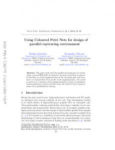
network layer. Furthermore, there is no preexisting infrastructure, such as base stations and routers, available. One of the challenges in ad-hoc networking is to design the routing protocols in such a way that they are able to quickly adapt to the frequent changes in network topology due to node mobility and nodes leaving/joining the network. Ad-hoc networking has a number of application areas, such as sensor networks, rescue operations in remote areas, mobile conferencing, home networking, and wireless personal area networks. Routing protocols for adhoc networking are under development by the IETF Mobile Ad-hoc Networks working group [35]. The main focus of the project is the integration of routing protocols for conventional wired data networks e.g, OSPF, RIP, and BGP [83]) with routing protocols for ad-hoc networks (e.g, DSR, AODV, and OLSR [71]). Figure 1 shows the IPv6 based network architecture considered in the project. The network architecture consists of an IPv6 core network connecting a number of mobile ad-hoc networks (MANETs) on the edge of the core network. The network architecture is aimed at supporting communication between nodes residing in different ad-hoc networks and communication between nodes in the ad-hoc networks and stationary nodes in the core network. Communication between nodes in the same ad-hoc network is facilitated by the ad-hoc network itself. Another important aspect of the network architecture is mobility. Macromobility is concerned with the movement of nodes from one ad-hoc network to another ad-hoc network, and the movement of an entire ad-hoc network from one point of attachment to the core network to another point of attachment. Micromobility is concerned with the movement of the nodes within an ad-hoc network which changes the topology of the ad-hoc network. Ad Hoc Network

Ad Hoc Network

Ad Hoc Network

Ad Hoc Network

IPv6 Core Network

Ad Hoc Network

Fig. 1. IPv6 based networking architecture.

CPN modelling was used in the first phase of the project to develop the network architecture shown in Fig. 1 and to capture in a rigorous way the communication and mobility scenarios that must be supported. Capturing these requirements was done by constructing a CPN model that described mobility and communication in the above networking architecture. In the following, we give a detailed description of this CPN model. 2.1

CPN Modelling of Mobility and Communication

Figure 2 shows the hierarchy page of the CPN model. The hierarchy page provides an overview of the pages (modules) constituting the CPN model and their


631

relationship. Each node in Figure 2 represents a page in the CPN model, and is labelled with a page name and a page number. As an example, the page node at the top left of Figure 2 is named Scenarios and has page number 1. Page Scenarios is the most abstract page in the CPN model. An arc between two nodes indicates that the destination page is a subpage (submodule) of the source page. The arc label(s) specifies the name of the substitution transition(s) representing the corresponding subpage at the source page. Substitution transitions are explained in more detail later.

Scenarios#1

M

Init#11

M

Hierarchy#100

C

Declarations#2

System

System#10

Enter

Enter#14 Exit

Exit#15 Mobility

Mobility#5 Macromobility

Macromobility#6

Type1

Type1#9

Type2

Type2#12

Type3

Type3#13 Micromobility

Micromobility#7 SendReceive1

Communication

SendReceive2

Communication#3

AHSendReceive

SendReceive4 SendReceive3 SendReceive

CNSendReceive#

Fig. 2. Hierarchy page - overview of CPN model.

The CPN model consists of three main parts. Page System and its two subpages model the system scenarios which are concerned with ad-hoc nodes entering and leaving the system. Page Mobility and its five subpages model the mobility scenarios, i.e., the movement of the nodes in the ad-hoc networks. Page Communication and its two subpages, AHSendReceive and CNSendReceive, model the communication between nodes in the system.

632


Figure 3 depicts page Scenarios which is the most abstract part of the CPN model. It corresponds to the Scenarios page node in Fig. 2. The rectangles in Figure 3 are substitution transitions as indicated by the associated HS-tag (in the lower left corner of each rectangle). Each substitution transition has an associated subpage modelling the compound behaviour represented by the substitution transition in more detail. The name of the subpage is given in the dashed box next to the HS-tag. The communication scenarios are modelled by the substitution transition Communication which has page Communication (see Fig. 2) as its associated subpage. The mobility scenarios are modelled by the substitution transition Mobility which has page Mobility as its associated subpage. The system scenarios are modelled by the substitution transition System which has page System as its associated subpage. 1‘CNnode(1)++ 1‘CNnode(2)++ 1‘CNnode(3)++ 1‘CNnode(4)++ 1‘CNnode(5) 5

1‘(AHnode(1),(Area1,IDLE))++ 1‘(AHnode(2),(Area1,IDLE)) 2

1‘(AHnode(3),(Area2,IDLE))++ 1‘(AHnode(4),(Area2,IDLE))

Core Network CNNode

Area1

2

AHNodexState

Area2

AHNodexState

Communication


HS

Communication#3 1‘AHnode(9)

Area3

Outside 1

AHNodexState


2

Area4

AHNodexState

AHNode

System HS

System#10

HS

Mobility#5

Mobility

Fig. 3. The Scenarios page - top level page in the CPN model.

The ellipses in Fig. 3 are called places and are used to model the state of the system. The state of a CPN model is called a marking and is a distribution of tokens on the places of the CPN model. Each of the places Area1, Area2, Area3, and Area4 correspond to areas where ad-hoc networks can exist. In our scenarios, ad-hoc networks can exist in four areas. Nodes that are part of the adhoc network in a given area are modelled as tokens residing on the corresponding place. The place CoreNetwork is used for modelling the nodes in the core network. The place Outside is used for modelling the ad-hoc nodes currently outside of the system.


633

The kind of tokens that may reside on a place is determined by the colour set of the place. A colour set in a CPN model is similar to a type in a programming language, and the values in a colour set are referred to as colours. The colour set of a place is typically written below the place and is declared using the Standard ML programming languages. As an example, place Area1 has the colour set AHNodexState. The declarations of the colour sets used in Fig. 3 are listed in Fig. 4 and will be explained below.

val AHn = 9; color AHInt = int with 1..AHn; color AHNode = union AHnode : AHInt; color Macrostate = with IDLE | MACROMOVE; color Area = with Area1 | Area2 | Area3 | Area4; color State = product Area * Macrostate; color AHNodexState = product AHNode * State; val CNn = 5; color CNInt = int with 1..CNn; color CNNode = union CNnode : CNInt;

Fig. 4. Colour sets used in Fig. 3.

The symbolic constant AHn is used to specify the total number of ad-hoc nodes in the system. Colour sets are declared using the keyword color. The colour set AHInt denotes the set of integers in the range from 1 to AHn. The colour set AHNode is used to model the ad-hoc nodes. An ad-hoc node is specified as a value (colour) with the form AHnode(i) where 1 ≤ i ≤ AHn. The colour set Macrostate is used to model the internal state of an ad-hoc node with respect to movement from one area to another area. The state may either be IDLE indicating that the node is currently not on the move from one area to another area, or MACROMOVE indicating that the node is currently on the move from one area to another area. The state of an ad-hoc node is modelled by the colour set State which is the cartesian product of the colour sets Area and Macrostate. Hence, the state of an ad-hoc node specifies the area that the ad-hoc node is currently in, and whether the ad-hoc node is currently moving from one area to another. The area places in Fig. 3 all have the colour set AHNodexState. Hence, tokens residing on these places represents ad-hoc nodes. Place Outside on page Scenarios has the colour set AHNode. The reason for this is that the state of the ad-hoc node is not important when the node is outside the system. The colour set CNNode is used to model the nodes in the core network. A core network node is specified as a value (colour) with the form CNnode(ci) where 1 ≤ bi ≤ CNn. Place CoreNetwork in Fig. 3 has the colour set CNNode.

634


The small circles and associated dashed boxes in Fig. 3 show the current marking of the CPN model. The small circle positioned inside a place indicates the number of tokens on the given place in the current marking. In the marking shown, there are two ad-hoc nodes in each of the four areas, and ad-hoc node 9 is currently outside the system. There are fives nodes in the core network. The dashed boxes positioned next to the places specify the colours of the individual tokens residing on that place. The marking of a place is a multi-set of tokens over the colour set of the place, i.e., there can be multiple appearances of the same token. The text inside the dashed boxes specifies the multi-set of tokens residing on the place using ++ to denote union (pronounced and) and ‘ (pronounced of) to specify coefficients, i.e., the number of occurrences of tokens with that value. As an example, on place Area1 in the marking shown in Fig. 3 there is one token of colour (AHnode(1),(Area1,IDLE)) and one token of colour (AHNode(1),Area1,IDLE). The CPN model contains an initialisation step responsible for the initial distribution of tokens on the CPN model. It is, however, possible for the modeller to also manually specify the initial marking of the CPN model. The transitions and places in Fig. 3 are connected by double-deaded arcs. Some of these arcs have been partly positioned on top of each other to improve readability of the figure. A place connected to a substitution transition is called a socket place, and a socket place is associated to a port place on the subpage associated with the substitution transition. This is called a port-socket assignment. This association has the effect that the port and the socket places will always have identical markings. Note that a place may be a socket place for several substitution transitions. The dynamics of a CPN model consists of occurrences of transitions (ordinary, not substitution transitions) which add and remove tokens to/from the places of the CPN model, thereby changing the current marking. An arc leading to a place from a substitution transition means that transitions on the subpage associated with the substitution transitions will add tokens on this place. Similarly, an arc leading from a place to a substitution transition means that transitions on the subpage will remove tokens from this place. A doubledeaded arc is a shorthand for an arc in each direction. The basic idea in the CPN model is to capture mobility scenarios of the network architecture by moving tokens corresponding to ad-hoc nodes from one area place to another area place. Similarly, communication scenarios will be modelled by moving tokens in the CPN model corresponding to packets. 2.2

Modelling Mobility

Figure 5 depicts page Mobility which is the most abstract page in the part of the CPN model specifying mobility. Two types of mobility are considered: macromobility and micromobility. Recall that macromobility is concerned with the mobility of ad-hoc nodes between ad-hoc networks. In the CPN model we consider only the macromobility case of one ad-hoc node moving from one ad-hoc network to another ad-hoc network. The case of an entire ad-hoc network moving can be viewed as the individual movement of all of the nodes in the ad-hoc network. Micromobility is concerned with the movement of ad-hoc nodes within


635

an ad-hoc network. The two types of mobility are modelled by the subpages of the substitution transitions Macromobility and Micromobility, respectively. The four places Area1-4 are port places of this page - indicated by the P-tags positioned next to them. The I/O-tag specifies that they are input and output port places. This means that tokens may be added and removed to/from these places. Each of the area places are associated with the identically named socket place in Fig. 3. The places Area1-4 are also socket places since they are connected to the Macromobility and Micromobility substitution transitions. 1‘(AHnode(3),(Area2,IDLE))++ 1‘(AHnode(4),(Area2,IDLE))


2

Area1

P

I/O

P

I/O

AHNodexState

Area2 2 AHNodexState

Macromobility 1‘(AHnode(5),(Area3,IDLE))++ 1‘(AHnode(6),(Area3,IDLE)) P

I/O

2

HS

Macromobility#6

Area3

AHNodexState


Area4 2 P I/O 1‘(Area1,[])++ 1‘(Area2,[])++ 1‘(Area3,[])++ 1‘(Area4,[])

AHNodexState

Microtopology 4 AreaxAHTopology

Micromobility HS

Micromobility#7

Fig. 5. The Mobility page.

The macromobility scenarios are specified by considering the movement of ad-hoc nodes between the places Area1-4. The place Microtopology is used to represent the current topology of the ad-hoc networks. The definition of the colour set AreaxAHTopology is given in Fig. 6.

color AHNodexAHNode = product AHNode * AHNode; color AHTopology = list AHNodexAHNode; color AreaxAHTopology = product Area * AHTopology;

Fig. 6. Declaration of colour set AreaxAHTopology.

The topology of an ad-hoc network is a pair consisting of the ad-hoc network and a list of pairs specifying the current set of links between the nodes in the ad-hoc network. For example, a pair (AHnode(6),AHnode(5)) captures that adhoc node 5 can be reached from ad-hoc node 6, but not necessarily the other way around as links may be unidirectional. In the current marking of place

636


Microtopology shown in Fig. 5, no ad-hoc nodes are able to reach each other in any area, and hence the topology in each area is specified as the empty list []. The substitution transition Macromobility is connected to the place Microtopology by a double arc. When a node moves from one area to another area, all existing links to nodes in the area being moved from disappear. Micromobility. Figure 7 depicts page Micromobility specifying the micromobility. The micromobility scenarios are abstractly modelled by viewing the ad-hoc network as a directed graph where edges represent connectivity. Hence, we have abstracted from the physical location of the nodes in the ad-hoc networks. The nodes in the ad-hoc networks are represented as tokens on the area places. The current topology of the ad-hoc network is represented by the tokens on place Microtopology. All five places on this page are connected via port-socket relationships to the identically named places on page Mobility (see Fig. 5). The two rectangles AddLink and DeleteLink are ordinary transitions. Transition AddLink models that a new link between two ad-hoc nodes arises, and transition DeleteLink models that an existing link between two ad-hoc nodes disappears.

1‘(Area1,[])++ 1‘(Area2,[])++ 1‘(Area3,[])++ 1‘(Area4,[]) (area, AddReach ahtopology (AHnode(i),AHnode(j))) P 1‘(AHnode(1),(Area1,IDLE))++ 1‘(AHnode(2),(Area1,IDLE)) P I/O

Area1 2

Microtopology 4 I/O

(area, DeleteReach ahtopology (AHnode(i),AHnode(j)))

AreaxAHTopology

if area = Area1 then (1‘(AHnode(i),statei) ++ 1‘(AHnode(j),statej)) else empty

AHNodexState 1‘(AHnode(3),(Area2,IDLE))++ 1‘(AHnode(4),(Area2,IDLE)) P I/O

Area2 2

(area, ahtopology)


(area, ahtopology)


Area3 2


Add Link

Delete Link


Area4

2


AHNodexState

[AHnode(i) AHnode(j), NotReach ahtopology (AHnode(i),AHnode(j))]

[Reach ahtopology (AHnode(i),AHnode(j))]

Fig. 7. The Micromobility page.

The actions of a CPN model consist of occurrences of enabled transitions removing tokens from places connected to incoming arcs and adding tokens to places connected to outgoing arcs of the transition. The transition AddLink is enabled in the marking shown in Fig. 7. This is indicated by the thick border of the transition. Transition AddLink has five input places and five output places. A transition is required to be enabled before it may occur. A transition is enabled


637

if sufficient tokens with adequate colours exist in each of its input places. When a transition occurs, it removes tokens from input places and adds tokens to output places. The exact multi-set of tokens required for a transition to be enabled and removed from input places when it occurs, and the exact multi-set of tokens added to output places of the transition are determined by assigning value to the variables of the transition, and by evaluating the arc expressions, i.e., the inscriptions positioned next to the arcs. Arc expressions are written in the Standard ML language. To evaluate the arc expressions on the surrounding arcs of a transition, a binding of the transition must be created. A binding is an assignment of data values to the variables of the transition. Figure 8 shows the declaration of the variables appearing in the surrounding arcs of the NewReach transition in Fig. 7. The definition of the colour sets have previously been given in Fig. 4.

var var var var

area i,j statei, statej ahtopology

: : : :

Area AHInt; State; AHTopology;

Fig. 8. Variables used on page Micromobility shown in Fig. 7.

A binding of a transition is enabled in the current marking if when evaluating each of the arc expressions on input arcs, the resulting multi-set of tokens is a subset of the multi-set of tokens currently present in the corresponding input place. An enabled binding of the transition AddLink is the following which lists the value assigned to each variable of the transition: < area=Area1,i=1, statei=IDLE, j=2, statej=IDLE, ahtopology=[] > This binding corresponds to the event that ad-hoc node 1 is now able to reach ad-hoc node 2. Evaluating the input arc expression from place Area1 in this binding yields the multi-set: 1‘(AHnode(1),IDLE) ++ 1‘(AHnode(2),IDLE). The result of evaluating the input arc expression from place Microtopology yields the multi-set 1‘(Area1,[]). The remaining input arc expressions all yield the empty multi-set since the variable area is bound to the value Area1. This binding is enabled since each of the multi-sets of tokens are present on the corresponding input places, and because the guard (shown in square bracket below the transition) of the NewReach transition is satisfied. A guard is a boolean expression that must evaluate to true in the binding in order for the transition to be enabled. The guard expresses the condition that the two ad-hoc nodes determined by the binding of the variables i and j must be distinct, and there must not already exist a link between ad-hoc node i and j. The latter requirement is checked by the function NotReach which is a function implemented in Standard ML. The implementation of the NotReach function is shown in Fig. 9. The implementation of the NotReach function uses the built-in Standard ML function [79] List.all to

638


check whether the edge between ad-hoc node i and j already exists in the list ahtopology corresponding to the current topology. We explain the other functions listed in Fig. 9 shortly.

fun NotReach ahtopology (ahnode1,ahnode2) = (List.all (fn edge => edge (ahnode1,ahnode2)) ahtopology) fun AddReach ahtopology (ahnode1,ahnode2) = (ahnode1,ahnode2)::ahtopology fun Reach ahtopology (ahnode1,ahnode2) = (List.exists (fn edge => edge = (ahnode1,ahnode2)) ahtopology) fun DeleteReach ahtopology (ahnode1,ahnode2) = List.filter (fn edge => edge (ahnode1,ahnode2)) ahtopology

Fig. 9. Function used in arc expression on page Micromobility in Fig. 7.

If the above enabled binding of transition AddLink occurs, it will remove the multi-set of tokens from input places of the transition obtained by evaluating the input arc expressions, and add the multi-set of tokens to each output place obtained by evaluating the corresponding output arc expression. Since the AddLink transition is connected to the area places with double arcs, the same multi-set of tokens will be removed and added for each of these places. Hence, the marking of these places will remain unchanged. The marking of place Microtopology will change as the token (Area1,[]) will be removed and a new token will be added as described by the arc expression from AddLink to Microtopology. This arc expression uses the function AddReach to add the edge AHnode(i),AHnode(j) to the microtopology in area 1. The AddReach function uses the list constructor :: to insert the edge (AHnode(i),AHnode(j)) at the head of the list ahtopology representing the current topology. Figure 10 shows the marking of page Micromobility after the occurrence of the above binding of the AddLink transition. The marking of the place Microtopology has changed so that Ahnode(1) is now able to reach AHnode(2) in area 1. The transition AddLink is also enabled in other bindings. In fact, it is enabled in bindings corresponding to all the possible edges that can arise between nodes given the current location of nodes in the four areas. In the marking shown in Fig. 10 both transitions are enabled. Transition DeleteLink is enabled with the binding: < area=Area1,i=1, j=2, ahtopology=[(AHnode(1),AHnode(2))] > The guard of the DeleteLink transition uses the function Reach to ensure that the transition is only enabled in bindings corresponding to links that exists in the area. The implementation of Reach is given in Fig. 9, and it uses the list library function List.exists to ensure that the link to be removed is an existing list in the current topology of the ad-hoc network. The output arc expression to

Application of Coloured Petri Nets in System Development 1‘(Area1,[(AHnode(1),AHnode(2))])++ 1‘(Area2,[])++ 1‘(Area3,[])++ 1‘(Area4,[]) (area, AddReach ahtopology (AHnode(i),AHnode(j)))

(area, DeleteReach ahtopology (AHnode(i),AHnode(j)))

Microtopology 4

P 1‘(AHnode(1),(Area1,IDLE))++ 1‘(AHnode(2),(Area1,IDLE)) P I/O

Area1

I/O

639

AreaxAHTopology


2 AHNodexState

1‘(AHnode(3),(Area2,IDLE))++ 1‘(AHnode(4),(Area2,IDLE)) P I/O

Area2 2

(area, ahtopology)


(area, ahtopology)


Area3

Delete Link

Add Link


2 AHNodexState

1‘(AHnode(7),(Area4,IDLE))++ 1‘(AHnode(8),(Area4,IDLE)) P I/O

Area4

2


AHNodexState

[AHnode(i) AHnode(j), NotReach ahtopology (AHnode(i),AHnode(j))]

[Reach ahtopology (AHnode(i),AHnode(j))]

Fig. 10. The Micromobility page - after occurrence of AddLink. P

I/O

Area1 2


AHNodexState P

I/O

Area2 2


AHNodexState 1‘(Area1,[(AHnode(1),AHnode(2))] )++ 1‘(Area2,[])++ 1‘(Area3,[])++ 1‘(Area4,[])

Type2

Type1 HS

Type1#9

HS

Type2#12

Type3 HS

Type3#13

Microtopology 4

P

I/O

AreaxAHTopology

P

I/O

Area3 2


AHNodexState P

I/O

Area4 2


AHNodexState

Fig. 11. The Macromobility page.

Microtopology uses the DeleteReach function to delete the edge in the list describing the topology in the area where the link disappears. If transition DeleteReach occurs in the above binding, it will result in the marking shown in Fig. 7. This means that it will remove the link which was added when AddLink occurred. Macromobility. Figure 11 depicts page Macromobility specifying the macromobility scenarios. Three types of macromobility are considered and modelled

640


by the subpages of the accordingly named substitution transitions. All arcs in Fig. 11 are double-headed arcs, but they have been positioned on top of each other to reduce the number of crossing arcs. Each of the three types of macromobility is described below. Type 1: This type specifies the movement of an ad-hoc node from one ad-hoc network to another ad-hoc network. The subpage Type1 modelling this type is shown in Fig. 12. The transition InstantMove represents the instantaneous move from one ad-hoc network to another ad-hoc network, i.e., at the same moment as the node leaves the ad-hoc network in one area it joins the ad-hoc network in another area. The declarations used are listed in Fig. 13. The value bound to the variable i (on the arcs between the area places and InstantMove) of type Int corresponds to the ad-hoc node that moves. When the InstantMove transition occurs, the variable to will be bound to the area which is being moved to and the variable from will be bound to the area being moved from. The microtopology of the area being moved from is also updated by changing the corresponding token [tofrom]

if (to = Area1) then 1‘(AHnode(i),(Area1,IDLE)) else empty if from = Area1 then 1‘(AHnode(i),(Area1,IDLE)) else empty

P

I/O


if (to = Area2) then 1‘(AHnode(i),(Area2,IDLE)) else empty

P

I/O

Area2 2 if from = Area2 then 1‘(AHnode(i),(Area2,IDLE)) else empty (from,DeleteAllReach ahtopology (AHnode(i)))

AHNodexState


P


Instant Move

(from, ahtopology)

Microtopology 4


P I/O

Area3 2


AHNodexState

I/O

AreaxAHTopology if (to = Area4) then 1‘(AHnode(i),(Area4,IDLE)) else empty

1‘(Area1,[(AHnode(1),AHnode(2))])++ 1‘( Area2,[])++ 1‘(Area3,[])++ 1‘(Area4,[])

if from = Area4 then 1‘(AHnode(i),(Area4,IDLE)) else empty

P I/O

Area4 2


AHNodexState

Fig. 12. Macromobility – Type 1.

var area,to,from : Area; var ahtopology : AHTopology; fun DeleteAllReach ahtopology ahnode = List.filter (fn (snode,dnode) => (snode ahnode) andalso (dnode ahnode)) ahtopology

Fig. 13. Declarations for macromobility – Type 1.


641

on place Microtopology. The function DeleteAllReach uses the built-in function List.filter to delete all edges in the microtopology related to the ad-hoc node that moves. An ad-hoc node has to be in its IDLE state to move from one area to another area. This ensures that the ad-hoc node is not currently moving according to one of the other types of macromobility types described below. The guard of the transition ensures that it is only enabled when the variables to and from are bound to different areas, i.e., the binding corresponds to movement of nodes between distinct areas. The following binding is an example of an enabled binding of the transition InstantMove in the marking shown in Fig. 14. It corresponds to the movement of ad-hoc node 1 from area 1 to area 2: < i=1,from=Area1,to=Area2,ahtopology=[AHnode(1),AHnode(2)] > The transition is enabled in bindings corresponding to all the possible movement of nodes between areas. An occurrence of the above binding results in the marking shown in Fig. 14 where the token corresponding to ad-hoc node 1 is now positioned on the place corresponding to area 2 and the link between ad-hoc nodes 1 and 2 in area 1 no longer exists. The movement of ad-hoc nodes is also evident on page Scenarios shown in Fig. 15. [tofrom]


if (to = Area2) then 1‘(AHnode(i),(Area2,IDLE)) else empty

P

I/O 1‘(AHnode(2),(Area1,IDLE))


P

I/O

Area2 3 if from = Area2 then 1‘(AHnode(i),(Area2,IDLE)) else empty (from,DeleteAllReach ahtopology (AHnode(i)))

(from, ahtopology)

P

AHNodexState

Instant Move if (to = Area3) then 1‘(AHnode(i),(Area3,IDLE)) else empty if from = Area3 then 1‘(AHnode(i),(Area3,IDLE)) else empty

Microtopology 4

1‘(AHnode(1),(Area2,IDLE))++ 1‘(AHnode(3),(Area2,IDLE))++ 1‘(AHnode(4),(Area2,IDLE))

P I/O

Area3 2


AHNodexState

I/O

AreaxAHTopology 1‘(Area1,[])++ 1‘(Area2,[])++ 1‘(Area3,[] )++ 1‘(Area4,[])


P I/O

Area4 2


AHNodexState

Fig. 14. Macromobility Type 1 - after occurrence of InstantMove.

Type 2: This type specifies the movement of an ad-hoc node from one ad-hoc network to another ad-hoc network. The difference between type 2 and type 1 is that there is a period of time in which the nodes moving are not part of any of the ad-hoc networks in Area1-4. The page for type 2 mobility is similar to the one for type 1 and is therefore omitted. Type 3: This type specifies the movement of an ad-hoc node from one ad-hoc network to another with the addition that there is a period of time in which

642

Lars Michael Kristensen, Jens Bæk Jørgensen, and Kurt Jensen 1‘CNnode(1)++ 1‘CNnode(2)++ 1‘CNnode(3)++ 1‘CNnode(4)++ 1‘CNnode(5) 5

1‘(AHnode(2),(Area1,IDLE))

1‘(AHnode(1),(Area2,IDLE))++ 1‘(AHnode(3),(Area2,IDLE))++ 1‘(AHnode(4),(Area2,IDLE))

Core Network CNNode

1

Area1

3

AHNodexState

Area2

AHNodexState

Communication


HS

Communication#3 1‘AHnode(9)

Area3

Outside 1

AHNodexState


2

Area4

AHNodexState

AHNode

System HS

System#10

HS

Mobility#5

Mobility

Fig. 15. The Scenarios page - after occurrence of InstantMove.

the node moving is part of both the ad-hoc network being moved from and the ad-hoc network being moved to. The page for type 3 mobility is similar to the one for type 1 and is therefore omitted. 2.3

Modelling Communication

Figure 16 depicts page Communication which is the most abstract page modelling the communication. The page models that each of the nodes (ad-hoc and core network nodes) may send and receive packets. Packets in transit between ad-hoc nodes are represented as tokens on place Routing. At the abstraction level of the CPN model, there is no distinction made between communication internally in an ad-hoc network and between nodes in different ad-hoc networks. The CPN model simply specifies the requirement that the packet must be delivered to the appropriate node - no matter in which ad-hoc network the node currently resides. Place Routing hence abstractly represents the routing functionality that will have to be implemented to get the packets from the source to the destination. How this is done is a design and implementation issue. The transition Drop Packet models that packets for ad-hoc nodes currently outside the system will be dropped. The declarations used for modelling communication between nodes are listed in Fig. 17. The colour set Packet is used modelling packets. A packet is abstractly represented as having a source and destination. As an example, a packet sent from AHnode(1) to AHnode(2) will be represented as a token with value (colour)

Application of Coloured Petri Nets in System Development 1‘CNnode(1)++ 1‘CNnode(2)++ 1‘CNnode(3)++ 1‘CNnode(4)++ 1‘CNnode(5)

1‘(AHnode(1),(Area1,IDLE))++ 1‘(AHnode(2),(Area1,IDLE)) P P

I/O

I/O

Area1 2

643


Core 5 Network 2

Area2

P

I/O

CNNode AHNodexState

AHNodexState

SendReceive SendReceive1 HS

HS

SendReceive2

CNSendReceive#16

AHSendReceive#4

HS

AHSendReceive#4

HS

AHSendReceive#4

Routing Packet

SendReceive3

SendReceive4

{src=node,dest=AHN(AHnode(i))} HS

AHSendReceive#4


Drop Packet


AHnode(i) P

I/O

Outside 1 P I/O


AHNode

1‘AHnode(9)

2

Area4

P

I/O

AHNodexState

Fig. 16. The Communication page.

color Node = union CNN : CNNode + AHN : AHNode; color Packet = record src : Node * dest : Node; var node : Node;

Fig. 17. Declarations for modelling communication.

{src = AHN(AHnode(1)), dest = AHN(AHnode(2))}. Hence for specification of requirements, we abstract from the actual content of packets. Page AHSendReceive modelling the sending and receiving of packets by adhoc nodes is shown in Fig. 18. It is the subpage of each of the four SendReceive1-4 substitution transitions in Fig. 16. This means that there will be four instances of this page when the CPN model is executed, one for each of the substitution transitions. The marking and enabling of transitions on these instances will be independent of each other. The instance depicted in Fig. 18 corresponds to the instance associated with the substitution transition SendReceive1 in Fig. 16. The transition SendPacket models the transmission of a packet from ad-hoc node i to a node assigned to the variable node. The transition ReceivePacket models the reception of a packet by ad-hoc node i. An occurrence of this transition will remove the token corresponding to the packet being received from place Routing. An occurrence of the SendPacket transition in Fig. 18 in a binding with: i=1, state=IDLE,dest=AHN(AHnode(3)) results in the marking shown in Fig. 19. The corresponding marking of page Communication is shown in Fig. 20. The ReceivePacket transition on the instance of the AHSendReceive page corresponding to the substitution transition SendReceive2 will now be enabled in binding corresponding to ad-hoc node 3 receiving the packet. The reception of the packet will result in the corresponding token being removed from place Routing.

644


P

Area 2

I/O

{src=AHN(AHnode(i)),dest=node}

Send Packet

(AHnode(i),state)


Routing

AHNodexState

P

I/O

Packet

Receive Packet

(AHnode(i),state)

{src=node,dest=AHN(AHnode(i))}

Fig. 18. The AHSendReceive page - instance for SendReceive1.

P

Area 2

I/O

{src=AHN(AHnode(i)),dest=node}

Send Packet

(AHnode(i),state)

1‘{src = AHN(AHnode(1)), dest = AHN(AHnode(3))}


1

Routing

AHNodexState

P

I/O

Packet

Receive Packet

(AHnode(i),state)

{src=node,dest=AHN(AHnode(i))}

Fig. 19. The AHSendReceive page - after occurrence of SendPacket. 1‘CNnode(1)++ 1‘CNnode(2)++ 1‘CNnode(3)++ 1‘CNnode(4)++ 1‘CNnode(5)

1‘(AHnode(1),(Area1,IDLE))++ 1‘(AHnode(2),(Area1,IDLE)) P P

I/O

I/O

Area1 2


Core 5 Network 2

Area2

P

I/O

CNNode AHNodexState

AHNodexState

SendReceive SendReceive1 HS

HS

SendReceive2

CNSendReceive#16 1‘{src = AHN(AHnode(1)), dest = AHN(AHnode(3))}

AHSendReceive#4

HS

AHSendReceive#4

HS

AHSendReceive#4

Routing 1 Packet

SendReceive3

SendReceive4

{src=node,dest=AHN(AHnode(i))} HS

AHSendReceive#4


Drop Packet


AHnode(i) P

I/O


Outside 1 P I/O AHNode

1‘AHnode(9)

2

Area4

P

AHNodexState

Fig. 20. Marking of the Communication page - packet in transit.

I/O


645

The modelling of send and receive for nodes in the core network is similar to the ad-hoc nodes. Hence, we do not give a detailed explanation of page CNSendReceive. 2.4

Conclusions on Modelling Ad-Hoc Networking Scenarios

The CPN model developed describes the abstract network architecture and associated communication and mobility scenarios considered in the project. A key point of the CPN model is that it captures the communication and the mobility aspects in a single model. The CPN model also allows derivation of combined scenarios involving simultaneously communication and mobility. As such, the CPN model can be seen as a formal documentation of the network architecture and its communication and mobility requirements. The CPN model is also suitable for generation of communication and mobility test-cases against which the later protocol designs can be checked. A number of such interesting scenarios were derived using simulation of the CPN model. The plan is to use these scenarios as test-cases for the protocols to be developed in later phases of the project. Finally, and probably most importantly, the development of the CPN model has served as an important tool for stimulating discussion of the network architecture and requirements. The graphical layout of the CPN model currently mimics the network architecture. This was chosen since it is easier to visualise the behaviour of the system directly at the level of the CPN model. This has been useful when presenting the CPN model to people without CPN knowledge. A more compact CPN model with tokens representing ad-hoc networks instead of tokens representing ad-hoc nodes could be developed. This would make it possible to model an arbitrary number of areas where ad-hoc networks can exists and it could be considered a more direct way of modelling mobility of an entire ad-hoc network. The CPN model would, however, lose some of its graphical appeal and hence possibly other means of graphics showing mobility and communication would have to be added to the CPN model. This approach seems more suitable for later CPN modelling of the actual protocol designs. The CPN model does not have an explicit representation of the connection between the core network and the ad-hoc networks since the purpose of the CPN model was to abstractly specify the communication and mobility requirements and scenarios related to nodes in the ad-hoc networks. The operation of gateways integrating the IPv6 core network routing protocols and the ad-hoc routing protocols is at a lower level of abstraction than the current CPN model. The purpose of the presented CPN model was to describe the scenarios and hence capture requirements in an implementation-independent manner.

3

Modelling Requirements in Pervasive Health Care

The pervasive health care system (PHCS) [12] is envisioned in a joint project between Aarhus County Hospital, the software company Systematic Software

646


Engineering A/S [84], and the Centre for Pervasive Computing [10] at the University of Aarhus. In this section, we describe how CP-nets are applied in requirements engineering for PHCS. The section is based on previous descriptions given in [52–54], and has benefitted from efforts of many participants in the pervasive health care research project [72]. The aim of PHCS is to improve the electronic patient record (EPR) [1], which is currently being deployed at the hospitals in Aarhus, Denmark. EPR is a comprehensive health care IT system with a budget of approximately 15 million US dollars; it will eventually have 8-10,000 users. EPR solves obvious problems occurring with paper-based patient records such as being not always up-to-date, only present in one location at a time, misplaced, and sometimes even lost. However, the version of EPR currently being deployed is a desktop PC based system which is not very practical for hospital work, since the users like nurses and doctors are often on the move and away from their offices (and, thus, desktop PCs). Moreover, users are frequently interrupted. Therefore, the desktop PC based EPR potentially induces at least two central problems for its users [6]. The first problem is immobility: in contrast to a paper-based record, an electronic patient record accessed only from desktop PCs cannot be easily transported. The second problem is time-consuming login and navigation: EPR requires user identification and login to ensure information confidentiality and integrity, and to start using the system for clinical work, a logged-in user must navigate, e.g., to find a specific document for a given patient. The motivation for PHCS is to address these problems. In the ideal situation, the users should have access to the IT system wherever they need it, and it should be easy to resume a work process which has previously been interrupted. 3.1

The Pervasive Health Care System

Use of personal digital assistants (PDAs), with which nurses and doctors could access EPR using a wireless network, is a possible solution to the immobility problem. That approach has been considered, but is not ideal, e.g., because of well-known characteristics of PDAs like small screens and limited memory, and because it does not fully address the time-consuming login and navigation problem. PHCS is a more ambitious solution which to a larger extent takes advantage of the possibilities of pervasive computing [81, 90]. Three basic design principles are exploited. The first principle is context-awareness [80]. This means that PHCS is able to register and react upon certain changes of context. More specifically, nurses, patients, beds, medicine trays, and other items are equipped with radio frequency identity (RFID) tags [74], enabling the presence of such items to be detected automatically by involved context-aware computers, e.g., located by the medicine cabinet and by the patient beds. The second design principle is that PHCS is propositional, in the sense that it makes qualified propositions, or guesses. Context changes may result in automatic generation of buttons that appear at the task-bar of computers. Users may explicitly accept a proposition by clicking a button – and implicitly ignore


647

or reject it by not clicking. The presence of a nurse holding a medicine tray for patient P in front of the medicine cabinet is a context that triggers automatic generation of a button Medicine plan:P, because in many cases, the intention of the nurse is now to navigate to the medicine plan for P. If the nurse clicks the button, she is logged in and taken to P’s medicine plan. It is, of course, impossible always to guess the intention of a user from a given context, and without the propositional principle, automatic shortcutting could become a nuisance since guesses would sometimes be wrong. The third design principle is that PHCS is non-intrusive, i.e., not interfering with or interrupting hospital work processes in an undesired way. Thus, when a nurse approaches a computer, it should react to her presence in such a way that a second nurse, who may currently be working on the computer, is not disturbed or interrupted. The last two design principles cooperate to ensure satisfaction of a basic mandatory user requirement: important hospital work processes have to be executed as conscious and active acts by responsible human personnel, not automatically by a computer. Figure 21 outlines PHCS (with an interface that is simplified and translated into English for the purpose of this paper). The current context of the system is that nurse Jane Brown is engaged in pouring medicine for patient Bob Jones for the giving to take place at 12 a.m. The medicine plan on the display shows which medicine has been prescribed (indicated by ‘Pr’), poured (‘Po’), and given (‘G’) at the current time. In this way, it can be seen that Advil and Tylenol have been poured for the 12 a.m. giving, but Comtrex not yet. Moreover, the medicine tray for another patient, Tom Smith, stands close to the computer, as can be seen from the task-bar buttons.

Fig. 21. PHCS – outline.

3.2

Medicine Administration

To aid requirements engineering for PHCS, CPN models of envisioned new work processes and of their proposed computer support were created. The scope of this section is the work process medicine administration, which is described below.

648


Assume that nurse N wants to pour medicine into a medicine tray and give it to patient P. First, N goes to the room containing the medicine cabinet (the medicine room). Here is a context-aware computer on which the buttons Login:N and Patient list:N appear on the task-bar when N approaches. If the second button is clicked, N is logged in and a list of those patients of which she is in charge is displayed on the computer. A medicine tray is associated with each patient. When N takes P’s tray nearby the computer, the button Medicine plan:P will appear on the task-bar, and a click will make P’s medicine plan appear on the display. N pours the prescribed medicine into the tray and acknowledges this in PHCS. When N leaves the medicine room, she is automatically logged out. N now takes P’s medicine tray and goes to the ward where P lies in a bed, which is supplied with a context-aware computer. When N approaches, the buttons Login:N, Patient list:N, and Medicine plan:P will appear on the task-bar. If the last button is clicked, the medicine plan for P is displayed. Finally, N gives the medicine tray to P and acknowledges this in PHCS. When N leaves the bed area, she is automatically logged out again. The given description captures just one specific combination of sub work processes. There are numerous other scenarios to take into account, e.g., medicine may be poured for one or more patients, for only one round of medicine giving, all four regular rounds of a 24 hours period, or for ad hoc giving; a nurse may have to fetch trays left at the wards prior to pouring; a nurse may approach the medicine cabinet without intending to pour medicine, but only to log into EPR (via PHCS) or to check an already filled medicine tray; two or more nurses may do medicine administration at the same time. To support a smooth medicine administration work process, the requirements for PHCS must deal with all these scenarios and many more. A CPN model, with its fine-grained and coherent nature, is able to support that.

3.3

Medicine Administration CPN Model

The medicine administration CPN model consists of 11 pages with a total of 54 places and 29 transitions. An overview of the model in terms of the hierarchy page is given in Fig. 22. The graph shows how the work process medicine administration is decomposed in sub-work processes. We give an impression of the model by describing the page shown in Fig. 23. The page models the pouring and checking of trays and is represented by the node PourChkTrays in Fig. 22. The medicine cabinet computer is in focus. It is modelled by a token on the Medicine cabinet computer place. This place has colour set COMPUTER, whose elements are 4-tuples (compid,display,taskbar,users) consisting of a computer identification, its display (main screen), its task-bar buttons, and its current users. In the initial marking, the computer has a blank display, no task-bar buttons, and no users. The colour set NURSE is used to model nurses. A nurse is represented as a pair (nurse,trays), where nurse identifies the nurse and trays is a container data structure holding the medicine trays that this nurse currently has in possession.

Application of Coloured Petri Nets in System Development MedAdm#1

Hierarchy#10

649

Erklaeringer#

GiveMed#7

GiveToPats#9

FindPlan#10

GetTrays#3

GiveToPat#1

PourChkTrays

PourChkTray

FindPlanTray#

PourAndAck#

ProvideTrays

Fig. 22. Medicine administration CPN model: hierarchy page.

Initially, the nurses Jane Brown and Mary Green are ready (represented as tokens in the Ready place) and have no trays. Occurrence of the Approach medicine cabinet transition models that a nurse changes from being ready to being busy nearby the medicine cabinet. At the same time, two buttons are added to the task-bar of the medicine cabinet computer, namely one login button for the nurse and one patient list button for the nurse. In the CPN model, these task-bar buttons are added by the function addMedicineCabinetButtons appearing on the arc from the transition Approach medicine cabinet to the place Medicine cabinet computer. The possible actions for a nurse who is by the medicine cabinet are modelled by the three transitions Pour/check tray, Enter EPR via login button, and Leave medicine cabinet. Often, a nurse at the medicine cabinet wants to pour and/or check some trays. How this pouring and checking is carried out is modelled on the subpage PourChkTray, which is the subpage of the substitution transition Pour/check tray. The Enter EPR via login button transition models that a nurse clicks on the login button and makes a general-purpose login to EPR. It is outside the scope of the model to describe what the nurse subsequently does – the domain of the model is specifically medicine administration, not general EPR use. The transition has a guard which checks if a nurse is allowed to log into EPR. When a nurse logs in, the login button for that nurse is removed from the task-bar of the computer, modelled by the removeLoginButton function. Moreover, the nurse is added to the set of current users by the function addUser. The Leave medicine cabinet transition models the effect of a nurse leaving: it is checked whether the nurse is currently logged in, modelled by the function

650

Lars Michael Kristensen, Jens Bæk Jørgensen, and Kurt Jensen (nurse,trays) (compid,display,taskbar,users)

Approach medicine cabinet

(compid,display, addMedicineCabinetButtons nurse taskbar, users)

(nurse,trays)

Pour/check HS tray

tray

1‘(janeBrown,noTrays)++ 1‘(maryGreen,noTrays)

By medicine cabinet

Ready 2 NURSE

NURSE

Trays by medicine cabinet TRAY

(nurse,trays) (nurse,trays) (compid,display,taskbar,users)

(nurse,trays)

Enter EPR via login button [loginAllowed nurse (compid,display, taskbar,users)]

Medicine cabinet 1 computer COMPUTER (compid,display, removeLoginButton nurse taskbar, addUser nurse users)

1‘(1,blank, noButtons, noUsers)

(compid,display,taskbar,users) Leave medicine cabinet (nurse,trays)

if loggedin nurse (compid,display,taskbar,users) then (compid, blank, removeMedicineCabinetButtons nurse taskbar, removeUser nurse users) else (compid, display, removeMedicineCabinetButtons nurse taskbar, users)

Fig. 23. Medicine administration CPN model: PourChkTrays page.

loggedin appearing in the if-then-else expression on the arc going from Leave medicine cabinet to the Medicine cabinet computer place. If the nurse is logged in, the medicine cabinet computer automatically returns to a blank screen, removes the nurse’s task-bar buttons (removeMedicineCabinetButtons), and logs her off (removeUser). If she is not logged in, the buttons generated because of her presence are removed, but the state of the computer is otherwise left unaltered. In any case, the token corresponding to the nurse is put back on the Ready place.

3.4

Medicine Administration Animation

An animation built on top of the CPN model is shown in Fig. 24. The animation is an interface to the CPN model, i.e., the animation is consistent with the CPN model and reflects the markings, transition occurrences, and marking changes that appear when the CPN model is executed. The animation hides the technicalities of CP-nets, e.g., concepts like places, transitions, tokens, enabling, occurrence, etc. In this way, the animation supports communication between users and system developers, by reducing the semantic distance [26] between the CPN model and the conception by the users of future work processes and their proposed computer support. The limitations of formal specifications as a means of communication in general, and, thus, the need for an animation, are widely recognised, see, e.g. [95]. The link between the CPN model and the animation is that the transitions of the CPN model are calling drawing functions related to the animation when

Application of Coloured Petri Nets in System Development Department

Bath

Ward

Team room

651

Provide trays

Ward Pour/check trays Give medicine

Ward

Medicine room

Ward

Bath

Medicine room Patient list: Jane Brown

Take tray

Login: Jane Brown

Leave medicine cabinet

Bob Jones

Ward

Fig. 24. Medicine administration animation.

they occur. Occurrence of a transition in this way triggers that graphical objects like nurse icons are created, moved, deleted, etc. in the animation. The animation runs in three windows. The Department window (at the top of Fig. 24) shows the layout of a hospital department with wards, the medicine room, the so-called team room (the nurses’ office), and two bathrooms. The Medicine room window (in the middle of Fig. 24) shows the medicine cabinet, pill boxes, tables, medicine trays, and the computer screen (enlarged). The Ward window (at the bottom of Fig. 24) shows a patient, a bed, a table, and the computer screen. Thus, the Department window gives an overview, and the other windows zoom in on areas of interest. The animation is interactive in the sense that the animation user is prompted to make choices. In Fig. 24, the animation shows a situation where nurse Jane Brown is in the medicine room, shown in the Department window and the Medicine room window, sufficiently close to produce two task-bar buttons at the computer. The animation user must make choices in order to drive the animation further. Specifically, by selecting one of the buttons to the right in the Medicine room window, the animation user can choose to take a tray or leave the medicine room. Also, the animation user can select one of the task-bar buttons at the computer. These four choices correspond to enabled transitions in the CPN model. As examples, if the animation user pushes the Leave medicine cabinet button, it forces the transition with the same name in the CPN model (cf. Fig. 23) to occur. The result of the occurrence is experienced by the animation user who sees Jane Brown walking away from the medicine cabinet and the removal of the task-bar buttons on the computer screen, which were generated because of

652


Jane Brown’s presence. If the animation user pushes the Take tray button and then selects Bob Jones’ medicine tray, it is moved close to the computer, and a medicine plan button for Bob Jones appears on the task-bar. If this button is pushed, the computer will display a screen similar to the one shown in Fig. 21. 3.5

CPN in Requirements Engineering for PHCS

The PHCS project started in early 2001. The first activities were domain analysis in the form of ethnographic field work, and a series of vision workshops with participation of nurses, doctors, computer scientists, and an anthropologist. An outcome of this analysis was natural-language descriptions of work processes and their proposed computer support. The first version of the CPN model presented in this section was based on these prose descriptions. The CPN model and the animation were extended and modified in a number of iterations, each version based on feedback on the previous versions. The animation has served as a basis for discussions in evaluation workshops with participation of nurses from hospitals in Aarhus and personnel from the involved software company. Through construction and use of the CPN model and the animation, in particular at the evaluation workshops, we have gained some experiences with CPnets in requirements engineering. In the terminology of [89], we have seen that for PHCS, the CPN model and the animation have been an effective means for specification, specification analysis, elicitation, and negotiation and agreement. Each of these concepts will be discussed in more detail below. Specification and Specification Analysis. Our specification has a sound foundation because of the formality and unambiguity of the CPN model. From the CPN model of medicine administration, requirements are precisely described by the transitions modelling manipulation of the involved computers. Each transition connected to the places modelling computers, e.g., the place Medicine cabinet computer shown in Fig. 23, must be taken into account. The following are examples of requirements induced by the transitions on the page of Fig. 23: 1. (R1) When a nurse approaches the medicine cabinet, the medicine cabinet computer must add a login button and a patient list button for that nurse to the task-bar (transition Approach medicine cabinet). 2. (R2) When a nurse leaves the medicine cabinet, if she is logged in, the medicine cabinet computer must return to a blank display, remove the nurse’s login button and patient-list button from the task-bar, and log her out (transition Leave medicine cabinet). 3. (R3) When a nurse selects her login button, she must be added as a user of EPR, and the login button must be removed from the task-bar of the computer (transition Enter EPR via login button). Specification analysis is well supported through simulation that allows experiments and trial-and-error investigations of various scenarios for the new envisioned work process. Specification analysis may also be supported through


653

formal verification. However, the CPN model of medicine administration is too large and complex to make, e.g., verification by exploration of the full state space possible in practice. In general, we believe that the full state space of a CPN model made to support requirements engineering typically will be very large. The reason is that often, in the view of the users who should be actively involved in the requirements engineering process, a representation of a work process and its proposed computer support must include many details. This conflicts with modelling the work process in a more coarse-grained, abstract way, with a corresponding smaller state space. Therefore, verification of CPN models supporting requirements engineering is an application area where strong methods for state space reduction, condensation, and exploration are highly needed. Elicitation. Elicitation includes the discovery of new requirements and the gain of a better understanding of known requirements. Elicitation is, like specification analysis, well supported through simulation. Simulation spurs elicitation by triggering many questions. Simulation of a CPN model typically catalyses the participants’ cognition and generates new ideas. Interaction with an executable model that is a coherent description of multiple scenarios most likely brings up questions, and issues appear that the participants had not thought about earlier. Examples of questions (Qs) that have appeared during simulation of the CPN model for medicine administration and corresponding answers (As) are: 1. (Q1) What happens if two nurses are both close to the medicine cabinet computer? (A1) The computer generates login buttons and patient list buttons for both of them. 2. (Q2) What happens when a nurse carrying a number of medicine trays approaches a bed? (A2) In addition to a login button and a patient list button for that nurse, only one medicine plan button is generated – a button for the patient associated with that bed. 3. (Q3) Is it possible for one nurse to acknowledge pouring of medicine for a patient while another nurse at the same time acknowledges giving of medicine for that same patient? (A3) No, that would require a more fine-grained concurrency control exercised over the patient records. Questions like Q1, Q2, and Q3 may imply changes to be made to the CPN model, because sometimes emergence of a question indicates that the current version of the CPN model does not reflect the work process properly. As a concrete example, in an early version of the medicine administration CPN model, the leaving of any nurse from the medicine cabinet resulted in the computer display being blanked off. To be compliant with the non-intrusive design principle for PHCS, the leaving of a nurse who is not logged in, should of course not disturb another nurse who might be working at the computer, and the CPN model had to be changed accordingly. Negotiation and Agreement. Leaving practical issues such as being widely accepted by involved stakeholders aside, negotiation and agreement may be eased

654


via CPN models. In large projects, negotiation about requirements inevitably takes place during the project. In many cases, this has strong economical consequences, because a requirements specification for a software system may be an essential part of a legal contract between a customer, e.g., a hospital, and a software company. Therefore, it is important to be able to determine which requirements were included in the initial agreement. Questions like Q1, Q2, and Q3 above may easily be subject to dispute. However, if the involved parties have the agreement that medicine administration should be supported, and have the overall stipulation that the formal and unambiguous CPN model is the authoritative description, many disagreements can quickly be settled. 3.6

Conclusions on Modelling Requirements to the PHCS

In this section, we have demonstrated that CPN models are able to support various common requirements engineering activities. However, of course, CPnets are not a panacea. Use of CP-nets does not address, e.g., how to carry out the necessary initial domain analysis, interviews with users, etc. Moreover, the purpose of the presented CPN model is solely to describe the requirements of an IT system, relative to the work processes to be supported. A number of other requirements issues are not addressed properly by the CPN model, e.g., performance and availability issues. The CPN model and the animation of the medicine administration work process can be seen as an alternative to or supplement to UML use cases [20,45]. Use cases model work processes to be supported by a new IT system, and a set of use cases is interpreted as functional requirements for that system. A main motivation for our choice of requirements engineering approach for PHCS was to build on top of prose descriptions of work processes and proposed computer support, consolidated as UML use cases, with which the stakeholders of PHCS were already familiar via EPR. A key observation, done many times before, is that UML use cases have a number of weaknesses and shortcomings, e.g., [82] points out a number of problems under headlines like use case modelling misses long-range logical dependency and use case dependency is non-logical and inconsistent. Various remedies have been proposed, see, e.g., [2, 3]. Having an executable representation of a work process, instead of a static representation in terms of a UML use case, supports specification analysis and elicitation as we discussed. This is possible via the CPN model itself, but can only be done properly by people who are able to read and understand the formal model. In practice, this often means only the system developers. The animation enables users like nurses and doctors to be actively engaged in specification analysis and elicitation, which is crucial. User participation increases the probability that a system is ultimately built that fits with the future users’ work processes.

4

State Space Analysis of an Audio/Video Protocol

Bang & Olufsen [5] is a Danish manufacturer of audio/video systems. The project described in this section was originally conducted in 1995-1996 [14] and was


655

concerned with the design of the next generation of the BeoLink system. The BeoLink system makes it possible to connect audio and video devices in a home via a dedicated network. The CPN modelling and analysis focused on the design of the lock management protocol in the BeoLink system. This protocol is used to grant devices exclusive access to services in the system, such as being able to use the loud speakers when playing music. The lock management protocol is based on the notion of a key, and a device is required to possess the key to access services in the system. When the system is switched on, exactly one key must be generated by the devices currently in the system. Furthermore, this key must be generated within 2 seconds for the system to be properly working. Special devices in the system called audio and video masters are responsible for generating the key when the system is switched on. A CPN model modelling BeoLink systems with 1-4 devices was constructed in the original project and analysed using the state space method of CP-nets. The CPN model constructed in the project was timed, meaning that the time taken by the various events in the lock management protocol was reflected in the CPN model. This was needed since the correctness of the lock management protocol depends on timing. When the project was conducted, the CPN computer tools had only support for ordinary state spaces, i.e., state spaces in their most basic form. Since the ordinary state space of the timed CPN model was infinite, this meant that only the initialisation phase of the lock management protocol could be validated. The initialisation phase is concerned with generating the key when the system is switched on. Since then, a number of more powerful state space methods have been developed and implemented in the CPN computer tools. In this section we give a brief presentation of a revised and more compact CPN model of the BeoLink system able to capture any number of devices. This is followed by a demonstration of how the more elaborate set of state space analysis methods currently available can be used to verify the full lock management protocol. 4.1

The Revised BeoLink CPN Model

Figure 25 shows the hierarchy page of the BeoLink CPN model. The subpage network models the network connecting the devices in the system. Page device and its subpages model the lock management protocol entities in each device. The subpages on the right, from reqkey down to fltimeo2 correspond to the different functional blocks of the lock management protocol. The subpage keyuser models the behaviour of devices as seen from the lock management protocol. Figure 26 shows the BeoLink page. The substitution transition Network represents the network connecting the devices in the system. The substitution transition Device models the devices in the system. The CPN model provides a folded representation of the behaviour of the devices. This is achieved by encoding the identity of the devices as part of the colour of tokens. This makes it possible to capture any number of devices without having to make changes to the net structure of the CPN model, and without having an instance of the subpages of the substitution transition Device for each of the devices in the system. This

656

Lars Michael Kristensen, Jens Bæk Jørgensen, and Kurt Jensen BeoLink#4 reqkey1#5 keywan1#6 newlock1#

device#43

LockMan#50

newlock2#

Hierarchy#

keylost1#5

decl#9990 keylost2#5 StateSpace keytran1#5 keyimp1#5 config#41 Debugging

keywan2#6

Generation

keyrel1#63

Verification fltimeo1#65 fltimeo2#66 network#42

keyuser#67

Fig. 25. Hierarchy page for the CPN BeoLink model.

Device HS

device#43

recbuf

c

TLG_BUFFERS

CONFIGS

sendbuf DIDxTLG_LIST

Network HS

network#42

Fig. 26. The BeoLink page.

way of compactly representating any number of devices, and which makes the CPN model parametric will become evident when we present the keyuser page. The socket places recbuf and sendbuf in Fig. 26 connecting the two substitution transitions, model send and receive message buffers between the devices and the network. Messages in the lock management protocol are called telegrams and are abbreviated TLG. Each device has a buffer for outgoing and incoming

Application of Coloured Petri Nets in System Development 1‘1@500++1‘2@[500]++1‘3@[500]

3

657

idle DIDT

1‘[(1,[]),(2,[]),(3,[])]

tlgbuf did

recbuf

1

P

I/O

TLG_BUFFERS 1‘(1,[])++ 1‘(2,[])++ 1‘(3,[])

(did,fl_cmd_list)

(did,tlg_list2)

requestkey

(did,fl_cmd_list^^[LOCK_MAN_KEY_WANTED])

fl_in

3

P

I/O

DIDxTLG_LIST 1‘(1,[])++ 1‘(2,[])++ 1‘(3,[])

did

sendbuf 3

P

I/O

(did,tlg_list3)

waiting

DIDxTLG_LIST DIDT

did

1‘(1,[])++ 1‘(2,[])++ 1‘(3,[])

fl_cmd_list 3

P

I/O

fl_status

DIDxFL_CMD_LIST

(did,KEY_IS_READY) P

In

getkey

DIDxFL_STATUS did@+(10+40*ran_0_1)

usekey DIDT did (did,fl_cmd_list^^[LOCK_MAN_KEY_RELEASE])

releasekey

(did,fl_cmd_list) did@+(10+40*ran_0_1)

Fig. 27. The keyuser page - initial marking.

telegrams. The place c is used for configuration of the CPN model and will not be explained in any detail. The behaviour of devices, as seen from the lock management protocol, is modelled by page keyuser shown in Fig. 27. Each device has a cyclic control flow where the device is initially idle (modelled by place idle), then it asks for the key (modelled by the transition requestkey), and it enters a state where it is waiting for the key (modelled by place waiting). Granting of the key to a device is modelled by the transition getkey which causes the device to enter a state where it is using the key (modelled by the place usekey). When the device is finished using the key, it will release the key and return to the idle state where it may then ask for the key again. The places fl status, fl cmd list, and fl in are used to model the internal state of a device. The places sendbuf and recbuf are linked to the accordingly named places on page BeoLink via port/socket relationship. The markings of these five places are also changed by the different functional blocks of the lock management protocol. Figure 27 shows a marking of the CPN model with three devices all in their idle state, as represented by the three tokens on place idle. A device is simply identified by a number. In the marking shown in Fig. 27 any of the three devices may ask for the key corresponding to the requestkey transition being enabled in three different bindings depending on the device identifier assigned to the variable did of colour set DIDT. The domain of the DIDT colour set is the set of device identifiers. If the transition occurs in a binding with did = 1, the token with colour 1 will be removed from place idle and added to place waiting. Figure 28 shows a marking of page keyuser where device 1 uses the key, whereas devices 2 and 3 have requested but have not been granted the key.

658

Lars Michael Kristensen, Jens Bæk Jørgensen, and Kurt Jensen idle DIDT

1‘[(1,[]),(2,[]),(3,[])]

tlgbuf

recbuf

did

1

P

I/O

TLG_BUFFERS 1‘(1,[])++ 1‘(2,[])++ 1‘(3,[])

(did,tlg_list2)

(did,fl_cmd_list)

fl_in

requestkey


3

I/O

1‘(1,[])++ 1‘(2,[])++ 1‘(3,[])

did

sendbuf 3 1‘2@[500]++1‘3@[500]

P

DIDxTLG_LIST

P

I/O

(did,tlg_list3) 2

waiting

DIDxTLG_LIST DIDT

did

1‘(1,[])++ 1‘(2,[])++ 1‘(3,[])

fl_cmd_list 3

P

I/O

fl_status


DIDxFL_CMD_LIST

In

getkey


usekey

1

1‘1@[2050]

DIDT did (did,fl_cmd_list^^[LOCK_MAN_KEY_RELEASE])

releasekey


Fig. 28. The keyuser page - device 1 using the key.

The CPN model of the BeoLink system is timed. This means that the CPN model captures the time taken by the different events in the protocol. The time concept of CP-nets is discrete and is based on the introduction of a global clock used to represent current model time. Furthermore, in addition to a data value, tokens in a timed CPN model may carry time stamps. The time stamp of a token describes the earliest model time at which the token can be consumed, i.e., removed by the occurrence of a transition. The time stamps of tokens are written as part of the current marking. As an example, the three tokens on place idle in Fig. 27 all have time stamp 500. This can be seen from the number in square brackets written after the @ sign in the box showing the details of the tokens residing on that place. To model that an event corresponding to the occurrence of a transition takes r time units, the tokens added to output places of the transition are given a time stamp that is r time units larger than the model time at which the transition occurs. The time units to add to the current model time when tokens are produced by the occurrence of a transition are specified using the @+ operator. As an example, the transition getkey uses the @+ operator in the arc expression on the output arc leading to the place usekey. The time units to add to the current model time is specified by the expression 10+40*ran 0 1 where ran 0 1 is a variable that can be bound to either 0 or 1. This models that the event of obtaining the key take either 10 or 50 time units. The execution of a timed CPN model is time driven. The CPN model remains at a given model time as long as there are enabled transitions at that model time. When no more transitions are enabled at the current model time, the global clock is incremented to the earliest next model time at which transitions are enabled. The model time in the marking shown in Fig. 27 is 500. Hence,


659

transition requestkey is enabled since the time stamps of the tokens on place idle are less than or equal to current model time. The model time in the marking shown in Fig. 28 is 2036. This is the reason why the releasekey transition is not enabled, since the time stamp of the token residing on place usekey is 2050. In the marking shown, transitions are enabled in the other pages of the CPN model. 4.2

Full State Spaces

The basic idea of state spaces is to calculate all reachable states and state changes of the system and represent these as a directed graph. The state space of a CPN model has a node for each of its reachable markings, i.e., markings that can be reached by occurrences of transitions starting from the initial marking. The outgoing arcs of a node n in the state space correspond to the set of enabled binding elements in that marking. A binding element is a pair consisting of a transition and an assignment of values to the variables of the transition. The destination node of an arc originating in node n is the node representing the marking resulting from the occurrence of the binding element corresponding to the arc in the marking represented by node n. idle

1

: 1‘1@[500]++1‘2@[500]++ 1‘3@[500] waiting : tempty usekey : tempty requestkey : did=1

requestkey : did=3 requestkey : did=2 idle

2

: 1‘1@[500]++ 1‘2@[500] waiting : 1‘3@[500] usekey : tempty

idle

3

requestkey : did=3

: 1‘1,@[500]++ 1‘3,@[500] waiting : 1‘2,@[500] use_key : tempty

idle

4

: 1‘2@[500]++ 1‘3@[500] waiting : 1‘1@[500] usekey : tempty

requestkey : did=1 requestkey : did=2

requestkey : did=2 keywan : did=2

6

7

keywan : did=3

keywan : did=1

10

5 requestkey : did=1


9

Fig. 29. Initial fragment of state space.

Figure 29 shows an initial fragment of the state space for the BeoLink system. Node 1 corresponds to the marking previously shown in Fig. 27. Figure 29 shows the nodes in the state space that are reachable by at most two occurrences of transitions starting from node 1. In the marking corresponding to node 1, there are three enabled binding elements corresponding to the three outgoing arcs from node 1. This three outgoing arcs correspond to all three devices being able to request the key in the marking corresponding to node 1. The dashed

660


boxes shown next to nodes 1-4 list the tokens present on selected places on the keyuser page in the marking represented by the node. The constant tempty denotes the empty set of tokens in a timed CPN model. These boxes have been omitted for some nodes to make the figure readable. The dashed boxes positioned on top of the arcs describes the enabled binding element to which the arc corresponds. The transition keywan is on another page in the CPN model. Figure 29 was created using the support in the CPN computer tools for drawing selected parts of a state space. The CPN computer tools make it possible to generate the state space manually as well as automatically. The state space can be generated either depth-first or breadth-first. From a constructed state space it is possible to automatically verify a number of properties of the system such as absense of deadlocks and other safety properties. The CPN computer tools contain a number of query functions that allow the analyst to investigate and verify the system using state spaces. The three main correctness criteria of the lock management protocol are listed below. 1. (C1) Key generation. When the system is booted, a key is eventually generated. The key is to be generated within 2.0 seconds. 2. (C2) Mutual exclusion. At any time during the operation of the system at most one key exists. 3. (C3) Key access. Any given device always has the possibility of obtaining the key, i.e., no device is ever excluded from getting access to the key. In the original analysis conducted in [14] only the first property was verified. The remaining properties could not be verified due to the state space of the timed CPN model being infinite. The key generation property was investigated by considering a partial state space, i.e., a finite fragment of the full state space. The partial state space was obtained by not generating successors for states where the key had been generated or where the model time had passed two seconds. It was then checked that in all markings for which successor states had not been generated, a key was present in the system. Table 1 lists some statistics showing the number of states in the partial state space and the CPU time it took to generate the partial state space. Configurations written with the form V M : n are configurations with a video master and a total of n devices. Similarly, configurations with one audio master and a total of n devices are written with the form AM : n. CPU time is written on the form h : mm : ss where h is Table 1. Statistics for partial state space of initialisation phase. Config Nodes AM : 3 1,839 AM : 4 22,675 AM : 5 282,399 VM : 3 1,130 VM : 4 13,421 VM : 5 164,170

Time 0:00:07 0:02:42 1:47:44 0:00:04 0:01:26 0:58:28


661

hours, mm is minutes, and ss is seconds. The results using partial state spaces and the revised CPN model were obtained on a HP Unix Workstation with 1 Gb of memory. 4.3

Timed Condensed State Spaces

A main problem with state spaces in their most basic form is that they are infinite for timed CPN models of cyclic/reactive systems. The problem is that the absolute notion of time as represented by the global clock and the time stamps of tokens are carried over into the state space. The BeoLink system is an example of a cyclic system since the devices are executing a loop where they request the key, are granted the key, and finally release the key. As a concrete example, consider the marking of the keyuser page shown in Fig. 30. This marking is similar to the marking previously shown in Fig. 28, except that all devices have had the key once and device 1 now possesses the key again. The markings in Fig. 28 and Fig. 30 are, however, represented by two nodes in the state space because the time stamps of the tokens and the value of the global clock differ. Intuitively, the markings are, however, similar. idle DIDT

1‘[(1,[]),(2,[]),(3,[])]

tlgbuf did

recbuf

1

P

I/O

TLG_BUFFERS 1‘(1,[])++ 1‘(2,[])++ 1‘(3,[])

(did,tlg_list2)

(did,fl_cmd_list)

requestkey


fl_in

3

I/O

1‘(1,[])++ 1‘(2,[])++ 1‘(3,[])

did

sendbuf 3 1‘2@[4372]++1‘3@[4472]

P

DIDxTLG_LIST

P

I/O

(did,tlg_list3) 2

waiting

DIDxTLG_LIST DIDT

did

1‘(1,[])++ 1‘(2,[])++ 1‘(3,[])

fl_cmd_list 3

P

I/O

fl_status

DIDxFL_CMD_LIST


In

getkey


usekey

1

1‘1@[4498]

DIDT did (did,fl_cmd_list^^[LOCK_MAN_KEY_RELEASE])

releasekey


Fig. 30. The keyuser page - all devices have used the key once.

Timed condensed state spaces [16] have been developed to overcome this problem, and use equivalence on the states to factor out the absolute notion of time. In this way, the infinite state space can be condensed into a finite state space. The condensed state space can be computed using a variant of the standard algorithm for state space construction, but without first constructing

662


the full state space. The basic idea is to normalise each state encountered during state space generation by: 1. (N1) Setting all time stamps on tokens that are less than current model time to zero (as their time stamp cannot influence enabling). 2. (N2) Subtracting the current model time from all time stamps of tokens that are greater than current model time. 3. (N2) Setting the current model time to 0. It have been proven [16] that all properties of the system expressible in the real-time temporal logic RCCTL∗ [31] are preserved in the condensed state space. This set of properties includes all standard dynamic properties of CP-nets. Table 2 shows statistics for the condensed state space for the full BeoLink system. The results were obtained on a HP Unix Workstation with 1Gb of memory. It was not possible to generate the time condensed state space for more than 3 devices with the available amount of memory. Using the condensed state space it is now also possible to verify properties C2 and C3 from Sect. 4.2. Property C2 can be expressed as the property that in no reachable marking is there more than one token on place usekey (see Fig. 27), and property C3 can be expressed as the property that from any reachable marking and for any device it is always possible to reach a marking where the token corresponding to this device is on place usekey. These two properties can be expressed using the query functions in the CPN state space tool and answers was computed in a few seconds. Table 2. Statistics for the time condensed state spaces. Config Nodes Arcs AM : 2 346 399 AM : 3 27,246 37,625 VM : 2 274 310 VM : 3 10,713 14,917

4.4

Time 0:00:03 0:04:10 0:00:02 0:01:34

The Symmetry Method

Many concurrent systems possess a certain degree of symmetry. For example, many concurrent systems are composed of similar components whose identities are interchangeable from a verification point of view. This symmetry is also reflected in the state spaces of such systems. The basic idea in the symmetry method [17, 19, 32, 43, 48, 49] is to represent symmetric states and symmetric binding elements using equivalence classes. State spaces can be reduced by factoring out this symmetry, and the symmetry-reduced state space is typically orders of magnitude smaller than the full state space. Furthermore, the same set of dynamic properties can be verified and analysed based on the symmetryreduced state space without unfolding to the full state space.


663

The devices in the BeoLink system that are not audio or video masters are symmetric, in the sense that they behave in the same way. They are only distinguishable by their device identity. This symmetry is also reflected in the state space (see Fig. 29). Consider, for instance, the two states 2 and 3 that correspond to states in which exactly one non-master device (device 1 is the audio master in the considered configuration) has requested the key. These two states are symmetric in the sense that node 2 can be obtained from node 3 by swapping the identity of device 2 and 3. Similarly, the two states represented by node 5 and node 10 can be obtained from each other by interchanging the identity of devices 2 and 3. These two states correspond to states in which one device has requested the key and the lock management protocol has registered the request. Furthermore, it can be observed that two symmetric states such as state 2 and state 3 have symmetric sets of enabled binding elements, and symmetric sets of successor states. This property can be extended to finite and infinite occurrence sequences of transitions. Figure 31 shows the initial fragment of the symmetry-reduced state space for the BeoLink system obtained by considering two states equivalent if one can be obtained from the other by a permutation of the identity of the non-master devices. The nodes and arcs now represent equivalence classes of markings and binding elements, respectively. The equivalence class of states represented by a node is listed in brackets in the inscription of the node, e.g., node 2 represents the states 2 and 3 from Fig. 29. A similar notation is used for binding elements. The basic idea in symmetry-reduced state spaces is to represent these equivalence classes by picking a representative for each equivalence class. The symmetries used to reduce the state space are required to be symmetries actually present in the CPN model. The CPN model is, therefore, required to satisfy a set of static properties relative to the set of symmetries to be used for the reduction [48]. 1 {1} {requestkey : did=2, requestkey : did=3}

{requestkey : did=1}

2 {2,3} {requestkey : did=2 requestkey : did=3}

3 {4} {requestkey : did=1} {requestkey : did=2 requestkey : did=3}

4 {6}

{keywan : did=2 keywan : did=3}

5 {5,10}

6 {7,9}

keywan : did=1

7 {8}

Fig. 31. Initial fragment of symmetry-reduced state space.

Table 3 shows the results when using the symmetry method on the initialisation phase of the BeoLink system. The size of the full state space for the

664

Lars Michael Kristensen, Jens Bæk Jørgensen, and Kurt Jensen Table 3. Statistics for symmetry reduced state space - initialisation phase.

Config AM : 3 AM : 4 AM : 5 AM : 6 VM : 3 VM : 4 VM : 5 VM : 6 VM : 7

Full State Spaces Nodes Time 1,839 0:00:07 22,675 0:02:42 282,399 1:47:44 3,417,719 1,130 0:00:04 13,421 0:01:26 164,170 0:58:28 1,967,159 22,892,208 -

Nodes 53.0 % 19.3 % 5.6 % 1.4 % 53.2 % 19.4 % 5.6 % 1.4 % 0.3 %

Symmetry Reduced Time Factor (n − 1)! 100.0 % 1.9 2 40.1 % 5.2 6 10.4 % 17.8 24 2:13:29 71.4 120 100.0 % 1.9 2 40.6 % 5.1 6 10.1 % 17.6 24 1:10:35 71.4 120 ≈15 hours 333.3 840

AM:6, VM:6, and VM:7 configurations has been calculated from the symmetryreduced state space by computing the size of each equivalence class. The results were obtained on a HP Unix Workstation with 1Gb memory. Calculation of the symmetry-reduced state space is based on calculating canonical representatives for each equivalence class [63]. This means that whenever a state is generated, this state is transformed into a canonical representative for its equivalence class. It is then checked whether this canonical representative is already included in the state space. The numbers in the Nodes column for the symmetry-reduced state space are relative to the number of nodes in the full state space, i.e., the number of nodes in the symmetry-reduced state space divided by the number of nodes in the full state space. The numbers in the Time column are also relative to the generation of the full state space for those configurations where the full state space could be generated. The Factor column gives the number of nodes in the full state space divided by the number of nodes in the symmetry reduced state space. The column (n− 1)! lists the factorial of n− 1 where n is the number of devices in the configuration. When there are n devices in the configuration, there are n − 1! possible permutations of the non-master devices. Hence, (n − 1)! is the theoretical upper limit on the reduction factor that can be obtained for a configuration with n devices. It can be seen that the computation time becomes large for 7 devices. This is due to the calculation of canonical representative being costly. It has been proven [17] that computing canonical representative for equivalence classes is at least as hard as the graph isomorphism problem for which no polynomial time algorithm is known. Table 4 lists the statistics for the symmetry-reduced state space of the full BeoLink system. Here we have used the symmetry method and the time condensed state space simultaneously. The number of nodes for the AM : 4 and V M : 4 configurations in the time condensed state space has been computed from the symmetry reduced state space. 4.5

The Sweep-Line Method

The amount of available main memory is often the limiting factor in the use of state spaces. During construction of the state space, the set of markings en-


665

Table 4. Statistics for symmetry reduced state space - full system.

Config AM : 2 AM : 3 AM : 4 VM : 2 VM : 3 VM : 4

Time Equivalence Nodes Time 346 0:00:03 27,246 0:04:10 12,422,637 274 0:00:02 10,713 0:01:34 3,557,441 -

Nodes 100.0 % 50.1 % 16.7 % 100. % 50.6 % 16.7 %

Symmetry Reduced Time Factor (n − 1)! 100.0 % 1 1 52.0 % 1.9 2 ≈25 hours 5.9 6 100.0 % 1 1 50.0 % 1.9 2 7:10:21 5.9 6

countered are kept in memory to recognise already visited marking and thereby ensure that the state space generation terminates. The basic idea of the sweepline method [15, 59] is to exploit a certain kind of progress exhibited by many systems. Exploiting progress makes it possible to explore all the reachable markings of a CPN model, while only storing small fragments of the state space in memory at a time. This means that the peak memory usage is reduced. The sweep-line method was used in [38] for verification of transactions in the Wireless Application Protocol (WAP) with a reduction in peak memory usage to 20%. The sweep-line method is aimed at on-the-fly verification of safety properties, e.g., determining whether a reachable marking exists satisfying a given state predicate. Hence, it can be used to verify properties C1 and C2 of the BeoLink system, but not property C3. The Basic Sweep-Line Method. For the BeoLink system, one source of progress is the time in the system (the model time) as represented by the value of the global clock in the CPN model. The global clock in a timed CP-net [48] has the property that for two markings M and M , where M is a successor marking of M , the value of the global clock in M is less than or equal to the value of the global clock in M . This progress can be formalised as a progress measure mapping a marking into the corresponding value of the global clock. The progress measure based on the global clock is a monotonic progress measure. Figure 32 shows how the markings/nodes in the state space fragment from Fig. 29 can be ordered according to this notion of progress. The intuition of the ordering is the following: markings in one layer all have the same value of the progress measure (the global clock), and markings in higher numbered layers are markings where the system has progressed further than in markings in lower numbered layers. Layer 0 contains markings in which the global clock has value 0. Layer 1 contains markings where the global clock is 500 time units. A marking in a given layer has successor markings either in the same layer or in a layer that represents further progress, but never in a layer that represents less progress. Markings in Layer 0 can thus never be reached by markings in Layer 1. If we calculate the markings one layer at a time, moving from one layer to the next when all markings in the first layer have been calculated and not before, we can think of it as a sweep-line moving through the state space. At any

666

Lars Michael Kristensen, Jens Bæk Jørgensen, and Kurt Jensen 1 requestkey : did=1

requestkey : did=3

Layer 0: Global clock 0

requestkey : did=2

2


4 requestkey : did=1 requestkey : did=2

requestkey : did=2 keywan : did=2

6

7

keywan : did=3

keywan : did=1

10



9 Layer 1: Global clock 500

Fig. 32. Initial fragment of full state space – arranged by progress.

one point during state space generation, the sweep-line corresponds to a single layer—all the states in the layer are “on” the sweep-line—and all new markings calculated are either on the sweep-line or in front of the sweep-line. Table 5 lists the statistics for the application of the sweep-line method on the initialisation phase of the BeoLink system and using the global clock as the progress measure. The figures in the Sweep-Line Method column are given relative to the numbers in the Full State Spaces columns. The results were obtained on a Pentium II PC with 160 Mb of memory. Table 5. Application of the sweep-line method – initialisation phase.

Config AM: 3 AM: 4 AM: 5 VM: 3 VM: 4 VM: 5

Full State Nodes 1,839 22,675 282,399 1,130 13,421 164,170

Spaces Time 0:00:11 0:05:32 5:03:53 0:00:06 0:02:40 2:30:27

Sweep-Line Peak Nodes 100.0 % 22.8 % 12.4 % 100.0 % 38.5 % 21.3 %

Method Time 100.0 % 84.0 % 39.4 % 100.0 % 106.0 % 45.4 %

The Generalised Sweep-Line Method. While the basic idea behind the sweep-line described above is intuitive and simple, it has the obvious drawback that it only works on systems exhibiting this kind of monotonic progress. While a lot of systems have a certain degree of progress, it is usually not strictly monotonic. There will be occasional occurrences of binding elements from highprogress markings to low-progress markings. The generalised sweep-line method [59] solves this problem by introducing multiple sweeps of the state space. Each


667

sweep follows only binding elements that result in markings with unchanged or increasing progress measure and collects information about regress-arcs that result in markings with decreasing progress measure. The markings at the end of regress-arcs are then marked as persistent meaning that they cannot be deleted again, and they are used as starting point for a subsequent sweep. The generalised sweep-line method visits all the reachable markings, but may visit some markings multiple times. To apply the sweep-line method for the full BeoLink system we first need to obtain a finite state space using the time condensed state spaces as described in Sect. 4.3. This, however, has the drawback that the value of the global clock becomes 0 in all markings. Hence, the progress measure defined above based on the global clock will map all markings into 0, resulting in no peak memory reduction when we apply the sweep-line method. It is however possible to define a non-monotonic progress measure for the BeoLink system based on the control flow of the devices. Recall that the devices have a cyclic control flow where they are first idle, then they request the key, and finally they obtain the key. When they have used the key they return to the idle state. This is a kind of local progress starting from the idle state progressing towards the state where they have the key. This ordering on the states of the devices can be used to define a non-monotonic progress measure. Details of such a progress measure can be found in [59]. With this progress measure, the marking shown in Fig. 28 will have a higher progress value than the marking shown in Fig. 27. When a device releases the key and moves to the idle state, then this will result in a regress-arc in the state space. Table 6 lists statistics for the application of the generalised sweep-line method to the full BeoLink system using the progress measure informally defined above. The experiments were conducted on a Pentium II PC with 160 Mb of memory. It can be seen that some states are explored multiple times which causes a time penalty, but the sweep-line method still achieves a reduction in peak memory usage to about 10 %. The relatively large time penalty is due to an inefficient implementation of deletion of states in the Design/CPN Sweep-Line Library [37]. A more efficient algorithm for deletion of states has been developed in [60]. Table 6. Application of the sweep-line method – full system.

Config AM:2 AM:3 VM:2 VM:3

Time Equivalence Nodes Time 346 00:02 27,246 06:54 274 00:02 10,713 02:19

Sweep-Line Method Nodes Explored Peak Nodes Time 102.6 % 18.8 % 200.0 104.1 % 9.7 % 327.8 103.3 % 15.0 % 200.0 106.3 % 9.7 % 207.2

% % % %

Above we have seen that it is possible to combine time condensed state spaces with both the symmetry method and the sweep-line method. It is also possible to use the sweep-line method and the symmetry method simultaneously. This

668


combination was investigated in [7] where it was demonstrated by means of experimental results that using the two methods simultaneously leads to better reduction than when either method is used in isolation. 4.6

Conclusions on Audio/Video Protocol and State Space Analysis

The revised state space analysis of the BeoLink system illustrates the use of the state space reduction methods that have been developed and implemented in the CPN computer tools in recent years. In addition to time condensed state spaces, the symmetry method, and the sweep-line method, several other methods have been developed to combat the state explosion problem. Examples of these include partial order reduction methods [70,87,93], the unfolding method [34,65], and methods based on Binary Decision Diagrams (BDDs) [66]. Until now, the above methods have only been used in practice on low-level Petri nets or by unfolding the high-level Petri net into the equivalent low-level Petri net. For CPN models constructed in industrial projects which often have variables from infinite domains, approaches based on unfolding to low-level are not feasible. Some work has been done on developing a version of the stubborn set method for CP-nets without having to rely on unfolding to low-level Petri net [56]. Methods that appear more promising for being included in the CPN computer tools include the bit-state hashing method [40, 41] and the state space caching method [39, 46] which both are based on ideas similar to the sweep-line method, i.e., deleting information about states during the state space exploration. In general, the CPN computer tools must support a suite of state space reduction methods since these reduction methods exploit different characteristics of the modelled system to achieve the reduction. As a consequence, only some reduction methods will work on a given CPN model. The protocol verification technique used, e.g., in [38] based on language comparison to verify a protocol specification against a service specification is another candicate for inclusion into the CPN computer tools. The support for state space methods in the CPN computer tools differs from other tools, such as SPIN [85], in its support for drawing selected parts of a state space and the support for a query language not based on temporal logic and model checking [18] but on functions to traverse the state space and extract information from the nodes and arcs. While it seldom makes sense to draw the full state space of a system, practical experience has shown that being able to visualise small fragments of the state space is an efficient way of investigating local behavior of the system in detail. A main reason for supporting a query language that allows the user to write traversals of the state space is that it provides better support for analysis. With the available query functions it is possible to compute quantitative values such as e.g., minimum and maximum number of tokens on a place rather than just yes/no answers as supported by temporal logic. Furthermore, query functions for typical dynamic properties of CPN models is also available. Instantiating these query functions is much more convenient for practitioners than writing the equivalent formulas in temporal logic. Support for CTL model checking [11] is, however, available as a library to the state space tool.


669

Another feature of the state space tool that has shown to be valuable in the practical use of state space methods is the support for generation of a predefined state space report. The state space report contains information regarding a set of standard dynamic properties of CP-nets and can be generated fully automatically and then inspected by the user. Generation of the state space report is usually the first activity in state space analysis, and many errors and problems in a design are often detectable from the state space report.

5

Implementation of a Planning Tool

This project [94] is concerned with the development of the Course of Action Scheduling Tool (COAST) by the Australian Defence Science and Technology Organisation (DSTO) [4]. A Course of Action (COA) (also referred to as a plan) consists of a set of tasks. The key capability of COAST is the computation of task schedules called line of operations (LOPs) and is aimed at supporting the planner in COA Development and COA Analysis which are two of the main activities in a military planning process. The basic idea in COAST is to use a CPN model for modelling the execution of tasks according to the pre- and postconditions of tasks, imposed synchronisations, and available resources. The LOPs are then obtained by generating a state space for the CPN model and extracting paths in the state space leading from the initial marking to certain markings representing end-states. The COAST planning tool has been developed in close cooperation with DSTO researchers, the Computer System Engineering Centre at University of South Australia [21], and planners at the Australian Defence Force. The latter group is the envisioned user of the tool. The role of CP-nets in the development of COAST has been threefold. Firstly, CPN modelling has been used in the development and specification of the underlying framework. Secondly, the constructed CPN model has been used directly in the implementation of COAST by embedding it into the COAST server which constitutes the computation back-end of COAST. Hence, CP-nets provide the semantical foundation by formalising and implementing the abstract conceptual framework underlying the tool. Finally, the analysis capabilities of COAST are based on state space methods. 5.1

An Example Plan

In this section we give a brief overview of the conceptual framework of the COAST and present a small example plan used as a running example throughout this section. The framework underlying COAST is based on four key concepts: Tasks are the basic units in a plan and have associated preconditions and effects describing the conditions required for a task to start and the effect of executing the task. A task also includes a specification of the resources required to execute the task, and may also have a specified duration. Tasks also have other attributes, but these are omitted in this presentation.

670


Conditions are used to describe the explicit logical dependencies between tasks via preconditions and effects. As an example, a task T1 may have an effect used as a precondition of a task T2. Hence, T2 logically depends on T1 in the sense that it cannot be started until T1 has been executed. Resources are used by tasks during their execution. Resources typically represent planes, ships, and personal required to executed a task. Resources may be available only at certain times due to e.g., service intervals. Resources may be lost in the course of executing a task. Synchronisation can be used to capture that a set of tasks must begin or end simultaneously, that there has to be a specific amount of time between the start and end of certain tasks, and that a task can only start after a certain point in time. A set of tasks that are required to begin at the same time is said to be begin-synchronised. A set of tasks required to end at the same time is said to be end-synchronised. End-synchronisations can cause the duration of tasks to be extended. Table 7 lists an example of a plan with 6 tasks. The table specifies for each task its preconditions, its effects, the required resources, and the duration of the tasks. In addition to the information provided in the table, the set {T5,T6} of tasks are begin-synchronised and the set {T4,T5,T6} of tasks are endsynchronised. The assigned resources are: 4’R1++3‘R2++3‘R3++1‘R5++1‘R6 (written as a multi-set). Figure 33 provides a graphical illustration of the dependencies between tasks using dashed lines to indicate begin-synchronisations and end-synchronisations. Table 7. A example plan with 6 tasks. Task T1 T2 T3 T4 T5 T6

Preconditions E1 E1 E1 E2 E3

Effects E1 E2 E3 E4 E5 E6

Resources Duration 4‘R1 2 2‘R2 ++ 2‘R3 4 2‘R2 ++ 2‘R3 7 1‘R2 ++ 1‘R3 1‘R5 7 1‘R6 7

For this example, we are interested in the possible ways (if any) that the set of tasks can be sequenced such that a state satisfying conditions E4, E5, and E6 can be reached given the assigned resources and synchronisation constraints. Figure 34 illustrates one such possible line of operation (LOP) by giving the start and end time of tasks such that the desired end-state is reached. 5.2

Engineering COAST

Figure 35 shows the client-server software architecture of COAST. The COAST client, which includes a domain-specific graphical user interface, is implemented

Application of Coloured Petri Nets in System Development begin

T2

E2

671

end

T5

E1

T1

E1

T3

E3

T6

E1

T4

Fig. 33. Illustration of dependencies between tasks in the example plan. T1 T2 T3 T4 T5 T6 0

2

6

Time

13

20

Fig. 34. One possible line of operation for the example plan.

in Java, whereas the COAST server is implemented in Standard ML (SML) via the embedded CPN model which forms the core of the COAST server. Communication between the client and the server is based on Comms/CPN and Comms/JAVA [36], a library supporting TCP/IP communication between CPN models and external applications. A SML session layer has been implemented on top of Comms/CPN. This layer allows the client to invoke functions available in the server and receive the corresponding results. The SML Session layer is implemented by allowing the client to submit SML code to the server for evaluation. The received SML code is then executed by the server, and results are sent back to the client. The SML code sent to the server corresponds to the invocation of the SML functions made available by the server by the COA Analysis module. The COAST client consists of two main parts: an Editor for creating and editing plans, and an Analyser for the analysis of plans. The COAST server consists of three main parts. The Initialisation module allows the CPN model to be initialised according to the plan to be analysed. The Simulation Code module for executing the CPN model which consists of the simulation code generated by the CPN computer tools for executing CPN models. The State Space Code and COA Analysis modules support the generation of state spaces and LOPs. The State Space Code module consists of the code for generation of state spaces in the CPN computer tools. Figure 36 is a snapshot from the COAST client illustrating how the user views the plans in the editor. There are four main windows. A window displaying the

672

Lars Michael Kristensen, Jens Bæk Jørgensen, and Kurt Jensen COAST Client

COAST Server COA Analysis

Analyser State Space Code Simulation Code

Editor

Initialisation SML Session

SML Session

Comms/Java

Comms/CPN TCP/IP

JAVA

Standard ML

Fig. 35. Architectural overview of the COAST tool.

Fig. 36. Snapshot from the COAST editor.

set of tasks, a window showing the assigned resources, and a window showing the conditions, and a window showing the synchronisations. Figure 37 shows an example of how LOPs are reported to the user in the Analyser part of the COAST client. The window gives a specification of the LOP


673

Fig. 37. Snapshot from the COAST analyser.

for the example plan corresponding to the one previously shown in Fig. 34. That the COAST server uses a CPN model as a basis for the scheduling analysis is fully transparent to the analyst using the COAST client.

5.3

The CPN Model

The CPN model has been parameterised with respect to the set of tasks, resources, conditions, and task synchronisations. This ensures that a given set of tasks, resources, and task synchronisation can be analysed by setting the initial marking of the CPN model accordingly, i.e., no changes to the structure of the CPN model are required to analyse a different set of tasks. Figure 38 shows the hierarchy page for the CPN model. The page CoastServer is the top level page in the CPN model which consists of three main parts. Page Execute (left) and its subpages model the execution of tasks, i.e, start, termination, abortion, and failure of tasks according to the set of tasks, resources, conditions, and synchronisation in the plan. Page Environment and its subpages model the environment in which tasks execute, and is responsible for managing the availability of resources over time, change of conditions over time, and task failures. Page Initialisation and its subpages are used for the initialisation of the model according to the concrete set of tasks, synchronisation, and resources in a plan. The CPN model

674

Lars Michael Kristensen, Jens Bæk Jørgensen, and Kurt Jensen CoastServer#20

Environment

Execute

Initialise

Environment#21

Initialisation#3

Execute#13 Start

Start#14

Resource Allocate

StartTasks

Terminate

Synchronisation

ResourceManager#19

Allocate#26 Change

StartTasks#2

VanConditions#22

Terminate#15

TaskFailure

Synchronisation#10

Resources

Conditions

TaskFailures#24

Normal

Resources#11

Conditions#16

Normal#28

Hierarchy#10010

Deallocate Failure

Deallocate#30

Fail

TaskFail#2

End

Failure#1

FailEndSynchronis Interrupt

Deallocate

FailDeallocate#8

TaskInterrupt#6

Interrupt Abort

Deallocate

IntDeallocate#4

End

Abort#7

AbortEndSynch#9

Fig. 38. Hierarchy page of the COAST CPN model.

is timed since capturing the time taken by executing a task is an important part of the computation of LOPs. The COAST server was obtained from the CPN model by first generating the standard simulation and state space code. SML files implementing Comms/CPN and the SML session layer were then loaded together with the functions implementing the server and the LOP generation algorithms. The resulting executable file constitutes the COAST server and includes the functions required to execute the CPN model and to conduct state space analysis. The COAST server is totally detached from the GUI of the CPN computer tools. When the COAST server is started, it will wait for an incoming TCP connection, and once the COAST client has established a connection, it can start invoking functions on the COAST server and thereby conduct the task scheduling analysis. Figure 39 shows the top level page of the CPN model with the three main parts of the CPN model represented as the substitution transitions Initialise, Execute, and Environment. The marking shown is the marking of the CPN model after initialisation of the CPN model with the example plan from Table 7. Place Tasks contains six tokens corresponding to the six tasks in the example plan. Place Conditions contains one token which is a list containing the conditions in the plan and their truth value. It can be seen that all conditions are initially false. Place Resources contains two tokens. There is one token consisting of a list describing the current set of idle (available) resources, and one token consisting of a list describing the resources that have been lost until now. Since the colour of the tokens on the places Resources and Tasks are of a complex colour set, we have not shown the detailed colours of the tokens but only the number of tokens. As an example, the colour set Task modelling tasks is record type with more than 15 fields.


675

e Init E

Initialise

Environment HS

Resources

2

Tasks 6 Task

Resources

Execute HS

Conditions 1 Conditions

HS

1‘[CONDITION(("E1",false)), CONDITION(("E2",false)), CONDITION(("E3",false)), CONDITION(("E4",false)), CONDITION(("E5",false)), CONDITION(("E6",false))]

Execute Status TaskxResxStatus

Fig. 39. The CoastServer page after initialisation. e Init E

Initialise

Environment HS

Resources Resources

2

Conditions 1

Tasks Task

Execute HS

Conditions

HS

1‘[CONDITION(("E1",true)), CONDITION(("E2",true)), CONDITION(("E3",true)), CONDITION(("E4",true)), CONDITION(("E5",true)), CONDITION(("E6",true))]

Execute 6 Status TaskxResxStatus

Fig. 40. The CoastServer page – all tasks executed.

Figure 40 shows the top level page of the CPN model in a marking where all six tasks in the example plan have been executed. All six tokens have been removed from place Tasks since the tasks have now been executed. The marking

676


shown corresponds to a desired end-state since the conditions E4, E5, and E6 are now all satisfied as can be seen from the marking of place Conditions. 5.4

Line of Operation Generation

The main analysis capability of COAST is the generation of LOPs. A LOP is a specification of start and end times for the tasks in the plan. The LOP generation implemented in the COAST server consists of two phases. In the first phase, the state space is generated relative to the plan to be analysed. Successors are not generated for states that qualify as desired end-states according to the conditions specified by the user. In the second phase, LOPs are computed by traversing the constructed state space. The LOPs are determined from the paths in the state space, and they are divided into two classes. Complete LOPs are LOPs that lead from the initial marking to a marking representing a desired end-state. The incomplete LOPs are LOPs that lead to markings representing undesired end-states, i.e., markings without enabled transitions that do not satisfy the conditions specified by the user. When incomplete LOPs are reported, the user will typically investigate the causes of these using queries about tasks, conditions, and resources in different states. In that sense, COAST also supports the planner in identifying errors and inconsistencies in the plan under analysis.

2

2

2

3

3

4

T4:2 3

3

3

7

4

4

5

8

4

4

5

9

6

10

T2:2 1

T1:2

T1:0 1

1

1

2

1

11

T2:2

T4:2 1

2

2

3

2

2

4

4

4

5

4

T3:2

T3:2

12

T4:2 2

T2:6 13

4

5

T3:6 3

6

6

6

15

5

5

6

6

6

T3:13 6

7

7

7

17

7

7

8

8

9

T5/T6:13 19

T2:9

T3:9 14

5

7

7

7

16

9

T2:13 8

8

8

8

18

8

8

8

1

1

9

9

T4/T5/T6:20 9

9

9

9

9

20

1

1

1

1

1

1

1

1

21

Fig. 41. State space for the example plan.

Figure 41 shows the state space for the example plan from Fig. 7. Node 1 to the left corresponds to the initial marking previously shown in Fig. 39. Node 21 to the lower right corresponds to the marking previously shown in Fig. 39. The


677

thick arcs in the state space correspond to start and termination of tasks. The other arcs correspond to internal events in the CPN model related to the start and termination of tasks. The thick arcs have labels of the form T i : t where i specifies the task number and t specifies the time at which the event takes place. As an example, task T1 starts at time 0 as specified by the label on the outgoing arc from node 1, and terminates at time 2 as specified by the label on the outgoing arc from node 2. The computation of LOPs is based on a breadth-first traversal of the state space starting from the initial marking. The basic idea is to compute the LOPs leading to each marking encountered during the traversal of the state space, where the LOPs in a given marking are computed from the LOPs associated with its predecessor markings. The LOPs associated with a given marking are then deleted once the LOPs have been computed for all its successor markings. The algorithm exploits the fact that the state space of the CPN model is acyclic for any plan, and that the paths leading to a given marking in the state space all have the same length measured in occuring binding elements. [(T1,0,2),(T2,2,?)] 2

2

2

3

3

4

T4:2 [(T1,0,2),(T2,2,?),(T4,2,?] 3

3

3

7

4

4

5

8

11

T2:2 T2:2 1

[]

T1:2

T1:0 1

1

1

[(T1,0,?)]

1

2

T4:2 1

2

2

[(T1,0,2)]

2

2

3

2

4

4

4

4

[(T1,0,2),(T4,2,?)] T3:2

[(T1,0,2),(T2,2,?),(T4,2,?]

5

[(T1,0,2),(T3,2,?),(T4,2,?] T3:2 4

4

5

9 12

T4:2 2

4

5

5

5

[(T1,0,2),(T3,2,?)]

6

6

6

6

10

[(T1,0,2),(T3,2,?),(T4,2,?]

Fig. 42. LOP generation after initial marking has been processed.

We now illustrate how the algorithm operates. Figure 42 shows the LOPs information associated with each marking in the first part of the state space. The LOP associated with the initial marking is the empty LOP represented as the empty list []. LOPs for the successor marking of the initial marking are now computed. Since the arc leading to the successor marking corresponds to the start of a task, the LOP is augmented with information about the time at which T1 was started. This results in the LOP: [(T1,0,?)] being associated with the successor marking of the initial marking. The LOP remains the same until the arc corresponding to the termination of T1 at time 2 is reached. In this case, the termination time of T1 can be recorded in the LOP. This results in associating the LOP [T1,0,2] with the successor marking of node 2. The LOP now associated with the succesor of node 2 is propagated forward. The LOP generation now proceeds and when node 3 is reached, the LOPs are propagated along three branches corresponding to the three successor markings of node 3. The LOP generation will now continue until the nodes 7, 8, 9, and 10 are reached. Here the LOPs associated with nodes 7 and 8 will be merged and associated with node 11 since the start and termination time of each of the tasks in the LOPs are identical. Similarly, the LOPs associated with node 9 and 10 will be merged

678


and associated with node 12. The breadth-first traversal will now continue until eventually the situation shown in Fig. 43 is reached where the two complete LOPs leading to the desired end-state have been computed. T4/T5/T6:20 9

9

9

9

9

20

1

1

1

1

1

1

1

1

1

1

21

[(T1,0,2),(T2,2,6),(T4,2,20),(T3,6,13),(T5,13,20),(T6,13,20)] [(T1,0,2),(T4,2,20),(T3,2,9),(T2,9,13),(T5,13,20),(T6,13,20)]

Fig. 43. Termination of the LOP generation.

Typical planning problems to which COAST is applied consist of 15 to 25 tasks resulting in state spaces with 10,000 to 20,000 nodes and 25,000 to 35,000 arcs. Such state spaces can be generated in less than 2 minutes on a standard PC. The state spaces are relatively small because the conditions, available resources, and imposed synchronisations in practice strongly limit the possible orders in which the tasks can be executed. 5.5

Conclusions on the Development of COAST

The development of the COAST tool is an example of how the usual gap between design as specified by a CPN model and the final implementation of a system can be overcome. The CPN model that was constructed to develop the conceptual and semantical foundation of COAST is being used directly in the final implementation of the COAST server. The project also demonstrates the value of having a full programming language environment in the form of the Standard ML compiler integrated in the CPN computer tools. The use of Standard ML as part of the CPN computer tools was crucial in several ways in the development of COAST. It allowed a highly compact and parameterisable CPN model to be constructed, and it allowed the CPN model to become the implementation of the COAST server. The parameterisation is important to ensure that the COAST server is able to analyse any set of tasks, resources, and synchronisations without having to make changes to the CPN model. Having a full programming language available also made it possible to extend the COAST server with the specialised algorithms required to extract the task schedules from a generated state space.

6

Conclusions and Future Directions

In this paper we have presented four projects where the CPN modelling language and computer tools have been put into practical use in system development projects. The project on modelling communication and mobility scenarios for ad-hoc networking illustrates how quite abstract CPN models can be used in an early phase of system development to determine the boundaries of the project and specify requirements. The pervasive health care project illustrated how CPnets can be used to construct an executable use case in the form of an animated


679

CPN model. An informal use case described in prose was augmented with notions of execution, formality, and animation. We have illustrated the use of state space methods for the analysis of the BeoLink system and for obtaining lines of operation in the COAST tool. The revised case study on the BeoLink system demonstrates that significant progress has been made in recent years on the support for state space analysis. The work presented on the COAST tool also shows how a CPN model can be integrated into an application making the use of CP-nets transparent to the user and overcoming the usual gap between design and implementation. Another example of automatic code generation from CPN models can be found in [67]. The paper [62] describes an approach to making a tailored graphical user interface on top of a CPN model using web technology. In general, many CPN projects have been carried out and documented in papers and reports. As examples, the proceedings of the CPN workshops 19982002 [51], and the two special issues of the Software Tools for Technology Transfer journal [27, 28] contain many papers on practical use of CP-nets. The most comprehensive overview of application and industrial use of CP-nets can be found on the web pages [22,23,25] that are maintained by our research group. Together, all these projects provide solid evidence that CP-nets have good potential to be used in the software industry. On the other hand, as evidenced by the recent survey [68], in general formal methods (like CP-nets) are only rarely used in the software industry. An interesting direction for future research is to try to increase the use of Petri nets in the software industry. That is for obvious reasons attractive for us as Petri net researchers. However, it may also be attractive for many parts of the software industry. It is widely recognised that today’s mainstream software development methods and tools are not always adequate for solving the range of difficult problems that software developers are facing. The choice of formal modelling language to be used in a system development project is non-trivial, and many aspects must be taken into account, e.g., available tool support and background of the involved system developers. Choosing CP-nets has a number of virtues. CP-nets has a sound, mathematically wellfounded execution semantics, is well-proven, and has proper tool support. This includes support for creating animations of CPN models, which has been used in a number of projects, see, e.g., [76] for an alarm system, [64] for mobile phones, and [8] for ISDN services. Even though we see a number of advantages of using Petri nets, other researchers and practitioners may have other opinions and preferences. If we want to advocate wide-spread and long-term use of Petri nets in system development in a company, we have to convince not only the software developers, but also higher-level decision makers like business and project managers. In conversations with the latter, we must stress the key business question: How does my company save time and money by using Petri nets? Sometimes, we should perhaps talk about reducing time to market, increasing return of investment, and limitation of risks, instead of about, e.g., nice theoretical properties like formal semantics. We should also promote Petri nets as a supplement to existing software development practices, not as something fundamentally new. In particular, with the success of UML, the software industry has in large scale adopted modelling as a

680


valuable discipline in everyday software development. Many software developers appreciate UML (in particular the static parts of UML such as class diagrams) as a productive asset to help them in their work. Those who have also tried to model behavioural aspects in UML might have encountered problems with UML state machines and activity diagrams. Therefore, for many developers, the motivation to use a supplementary modelling language together with UML may be quite high. In this way, the success of UML can be seen as a good chance to establish Petri nets more broadly in the software industry. The reader interested in getting started with CPN modelling is referred to the paper [58] and the book [47]. The paper introduces the CPN modelling language using a simple communication protocol, whereas the book contains several smaller examples and also the formal definition of CP-nets. Readers interested in getting started using the state space method is referred to the book [48], the introductory paper [58], and the examples found on the web pages [22, 25]. The reader interested in the recent work on state space methods is referred to [16] for the time condensed state spaces, [15, 59] for the sweep-line method, and [29] for the symmetry method. CPN models can also be analysed using simulation, and the papers [91,92] describe how quantitative measures such as throughput and delay of the system can be obtained using simulation-based performance analysis and the CPN computer tools. The web pages for the CPN computer tools [22, 25] contain several tutorials and small examples of CPN models useful for getting started using CPN modelling and the CPN computer tools. A license for the CPN computer tools can be obtained free of charge, and a licence form is available electronically from our web-pages [22]. Mailing lists have also been established for users of the CPN computer tools.

References 1. Aarhus Amt Electronic Patient Record. www.epj.aaa.dk. 2. D. Amyot, R.J.A. Buhr, T. Gray, and L. Logrippo. Use Case Maps for the Capture and Validation of Distributed Systems Requirements. In Proc. of 4th IEEE International Symposium on Requirements Engineering, pages 44–53. IEEE Computer Society, 1999. 3. A.I. Ant´ on, R.A. Carter, A. Dagnino, J.H. Dempster, and D.F. Siege. Deriving Goals from a Use-Case Based Requirements Specification. Requirements Engineering Journal, 6:63–73, 2001. Springer-Verlag. 4. Australian Defence Science and Technology Organisation. www.dsto.defence.gov.au. 5. Bang & Olufsen. www.bang-olufsen.com. 6. J.E. Bardram and C. Bossen. Moving to get aHead: Local Mobility and Collaborative Work. In Proc. of 8th European Conference on Computer-supported Cooperative Work, pages 355–374. Kluwer Academic Publishers, 2003. 7. J. Billington, G. Gallasch, L.M. Kristensen, and T. Mailund. Exploiting Equivalence Reduction and the Sweep-Line Method for Detecting Terminal States. IEEE Transactions on Systems, Man, and Cybernetics. Part A: Systems and Humans, 2004. To appear.


681

8. C. Capellmann, S. Christensen, and U. Herzog. Visualising the Behaviour of Intelligent Networks. In Services and Visualisation, Towards User-Friendly Design, volume 1385 of Lecture Notes in Computer Science, pages 174–189. Springer-Verlag, 1998. 9. ITU (CCITT). Recommendation Z.120: MSC. Technical report, International Telecommunication Union, 1992. 10. Centre for pervasive computing. www.pervasive.dk. 11. A. Cheng, S. Christensen, and K.H. Mortensen. Model Checking Coloured Petri Nets Exploiting Strongly Connected Components. In Proc. of the International Workshop on Discrete Event Systems, WODES96. Institution of Electrical Engineers, Computing and Control Division, Edinburgh, UK, 1996. 12. H.B. Christensen and J.E. Bardram. Supporting Human Activities – Exploring Activity-Centered Computing. In Proc. of 4th Ubicomp Conference, volume 2498 of Lecture Notes in Computer Science. Springer-Verlag, 2002. 13. S. Christensen. Message Sequence Charts. User’s Manual, January 1997. 14. S. Christensen and J.B. Jørgensen. Analysis of Bang and Olufsen’s BeoLink Audio/Video System Using Coloured Petri Nets. In Proc. of 18th International Conference on Application and Theory of Petri Nets, volume 1248 of Lecture Notes in Computer Science, pages 387–406. Springer-Verlag, 1997. 15. S. Christensen, L.M. Kristensen, and T. Mailund. A Sweep-Line Method for State Space Exploration. In Proc. of 7th International Conference on Tools and Algorithms for the Construction and Analysis of Systems, volume 2031 of Lecture Notes in Computer Science, pages 450–464. Springer-Verlag, 2001. 16. S. Christensen, L.M. Kristensen, and T. Mailund. Condensed State Spaces for Timed Petri Nets. In Proc. of 22nd International Conference on Application and Theory of Petri Nets, volume 2075 of Lecture Notes in Computer Science, pages 101–120. Springer-Verlag, 2001. 17. E. Clarke, E.A. Emerson, S. Jha, and A.P. Sistla. Symmetry Reductions in Model Checking. In Proc. of 10th International Conference on Computer-Aided Verification, volume 1427 of Lecture Notes in Computer Science, pages 147–159. SpringerVerlag, 1998. 18. E. Clarke, O. Grumberg, and D. Peled. Model Checking. The MIT Press, 1999. 19. E.M. Clarke, R. Enders, T. Filkorn, and S. Jha. Exploiting Symmetries in Temporal Logic Model Checking. Formal Methods in System Design, 9(1/2):77–104, 1996. 20. A. Cockburn. Writing Effective Use Cases. Addison-Wesley, 2000. 21. Computer Systems Engineering Centre at University of South Australia. www.unisa.edu.au/eie/csec/. 22. CPN Tools. www.daimi.au.dk/CPNtools. 23. The CPN Group at University of Aarhus. www.daimi.au.dk/CPnets. 24. J. Desel and W. Reisig. Place/Transition Petri Nets. In Lecture on Petri nets I: Basic Models, volume 1491 of Lecture Notes in Computer Science, pages 122–173. Springer-Verlag, 1998. 25. Design/CPN. www.daimi.au.dk/designCPN. 26. N. Dulac, T. Viguier, N. Leveson, and M.-A. Storey. On the Use of Visualization in Formal Requirements Specification. In Proc. of 7th IEEE International Symposium on Requirement Engineering, pages 71–80. IEEE Computer Society, 2002. 27. K. Jensen (ed.). International Journal on Software Tools for Technology Transfer, Vol. 2, No. 2. Special section on Coloured Petri nets, 1998. 28. K. Jensen (ed.). International Journal on Software Tools for Technology Transfer, Vol. 3, No. 4. Special section on Coloured Petri nets, 2001.

682


29. L. Elgaard. The Symmetry Method for Coloured Petri Nets. PhD thesis, Department of Computer Science, University of Aarhus, July 2002. 30. M. Elkoutbi and R.K. Keller. User Interface Prototyping Based on UML Scenarios and High-Level Petri Nets. In Proc. of 21st International Conference on Application and Theory of Petri Nets, volume 1825 of Lecture Notes in Computer Science. Springer-Verlag, 2000. 31. E. A. Emerson, A.K. Mok, A.P Sistla, and J. Srinivasan. Quantitative Temporal Reasoning. In Proc. of 2nd International Workshop on Computer-Aided Verification, volume 531 of Lecture Notes in Computer Science, pages 136–145. SpringerVerlag, 1990. 32. E.A. Emerson and A.P. Sistla. Symmetry and Model Checking. Formal Methods in System Design, 9(1/2):105–131, 1996. 33. Ericsson Telebit A/S. www.ericssontelebit.dk. 34. J. Esparza. Model Checking using Net Unfoldings. Science of Computer Programming, 23:151–195, 1994. 35. Internet Engineering Task Force. Mobile ad-hoc networks. www.ietf.org/html.charters/manet-charter.html. 36. G. Gallasch and L. M. Kristensen. Comms/CPN: A Communication Infrastructure for External Communication with Design/CPN. In Proc. of the 3rd Workshop and Tutorial on Practical Use of Coloured Petri Nets and the CPN Tools, pages 79–93. Department of Computer Science, University of Aarhus, 2001. DAIMI PB-554. 37. G.E. Gallasch, L.M. Kristensen, and T. Mailund. Sweep-Line State Space Exploration for Coloured Petri Nets. In Proc. of 4th Workshop and Tutorial on Practical Use of Coloured Petri Nets and the CPN Tools, pages 101–120. Department of Computer Science, University of Aarhus, 2002. DAIMI PB-560. 38. S. Gordon, L.M. Kristensen, and J. Billington. Verification of a Revised WAP Wireless Transaction Protocol. In Proc. of 23rd International Conference on Application and Theory of Petri Nets, volume 2360 of Lecture Notes in Computer Science, pages 182–202. Springer-Verlag, 2002. 39. G.J. Holzmann. Tracing Protocols. Bell System Technical Journal, 64:2413–2434, 1985. 40. G.J. Holzmann. Design and Validation of Computer Protocols. Prentice-Hall International Editions, 1991. 41. G.J. Holzmann. An Analysis of Bitstate Hashing. Formal Methods in System Design, 13(3):287–305, 1998. 42. C. Huitema. IPv6: The New Internet Protocol. Prentice-Hall, 1998. 43. C.N. Ip and D.L. Dill. Better Verification Through Symmetry. Formal Methods in System Design, 9(1/2):41–75, 1996. 44. M. Jackson. System Development. Prentice-Hall, 1983. ¨ 45. I. Jacobson, M. Christerson, P. Jonsson, and G. Overgaard. Object-Oriented Software Engineering: A Use Case Driven Approach. Addison-Wesley, 1992. 46. C. Jard and T. Jeron. Bounded-memory Algorithms for Verification On-the-fly. In Proc. of 3rd International Workshop on Computer-Aided Verification, volume 575 of Lecture Notes in Computer Science, pages 192–202. Springer-Verlag, 1991. 47. K. Jensen. Coloured Petri Nets - Basic Concepts, Analysis Methods and Practical Use. - Volume 1: Basic Concepts. Springer-Verlag, 1992. 48. K. Jensen. Coloured Petri Nets - Basic Concepts, Analysis Methods and Practical Use. - Volume 2: Analysis Methods. Springer-Verlag, 1995. 49. K. Jensen. Condensed State Spaces for Symmetrical Coloured Petri Nets. Formal Methods in System Design, 9(1/2):7–40, 1996.


683

50. K. Jensen. Coloured Petri Nets - Basic Concepts, Analysis Methods and Practical Use. - Volume 3: Practical use. Springer-Verlag, 1997. 51. K. Jensen, editor. Proceedings Workshop and Tutorial on Practical Use of Coloured Petri Nets and CPN Tools. Available via www.daimi.au.dk/CPnets, 1998-2002. 52. J.B. Jørgensen. Coloured Petri Nets in Development of a Pervasive Health Care System. In In Proc. of 24th International Conference on Application and Theory of Petri Nets, volume 2679 of Lecture Notes in Computer Science, pages 256–275. Springer-Verlag, 2003. 53. J.B. Jørgensen and C. Bossen. Requirements Engineering for a Pervasive Health Care System. In Proc. of 11th IEEE International Requirements Engineering Conference, pages 55–64. IEEE Computer Sociery, 2003. 54. J.B. Jørgensen and C. Bossen. Executable Use Cases: Requirements for a Pervasive Health Care System. IEEE Software, March/April 2004. To appear. 55. J.B. Jørgensen and S. Christensen. Executable Design Models for a Pervasive Healthcare Middleware System. In In Proc. of the 5th UML Conference, volume 2460 of Lecture Notes in Computer Science, pages 140–149. Springer-Verlag, 2002. 56. L. M. Kristensen and A. Valmari. Finding Stubborn Sets of Coloured Petri Nets Without Unfolding. In Proceedings of 19th International Conference on Application and Theory of Petri Nets, volume 1420 of Lecture Notes in Computer Science, pages 104–123. Springer-Verlag, 1998. 57. L.M. Kristensen. Ad-hoc Networking and IPv6: Modelling and Validation. www.pervasive.dk/projects/IPv6/IPv6_summary. 58. L.M. Kristensen, S. Christensen, and K. Jensen. The Practitioner’s Guide to Coloured Petri Nets. International Journal on Software Tools for Technology Transfer, 2(2):98–132, 1998. 59. L.M. Kristensen and T. Mailund. A Generalised Sweep-Line Method for Safety Properties. In Proc. of Formal Methods Europe, volume 2391 of Lecture Notes in Computer Science, pages 549–567. Springer-Verlag, 2002. 60. L.M. Kristensen and T. Mailund. A Compositional Sweep-Line State Space Exploration Method. In Proc. of Formal Techniques for Networked and Distributed Systems, volume 2529 of Lecture Notes in Computer Science, pages 327–343. SpringerVerlag, 2002. 61. P. Kruchten. The Rational Unified Process: An Introduction. Addison-Wesley, 1999. 62. B. Lindstrøm. Web-Based Interfaces for Simulation of Coloured Petri Net Models. International Journal on Software Tools for Technology Transfer, 3(4):405–416, 2001. 63. L. Lorentsen and L. M. Kristensen. Exploiting Stabilizers and Parallelism in State Space Generation with the Symmetry Method. In Proceedings of International Conference on Application of Concurrency in System Design, pages 211–220. IEEE Computer Society, 2001. 64. L. Lorentsen, A-P Tuovinen, and J. Xu. Modelling Features and Feature Interactions of Nokia Mobile Phones Using Coloured Petri Nets. In Proc. of the 23rd International Conference on Application and Theory of Petri Nets, Lecture Notes in Computer Science. Springer-Verlag, 2002. 65. K. L. McMillan. A Technique of State Space Search Based on Unfolding. Formal Methods in System Design, 6(1):45–65, 1995. 66. K.L. McMillan. Symbolic Model Checking. Kluwer Academic Publishers, 1993. 67. K.H. Mortensen. Automatic Code Generation Method Based on Coloured Petri Net Models Applied on an Access Control System. In Proceedings of 21st International Conference on Application and Theory of Petri Nets, volume 1825 of Lecture Notes in Computer Science, pages 367–386. Springer-Verlag, 2000.

684


68. C.J. Neill and P.A. Laplante. Requirements Engineering: The State of the Practice. IEEE Software, 20(6):61–69, 2003. 69. OMG Unified Modeling Language Specification, Version 1.4. Object Management Group (OMG); UML Revision Taskforce, 2001. 70. D. Peled. All from One, One for All: On Model Checking Using Representatives. In Proc. of 5th International Conference on Computer-Aided Verification, volume 697 of Lecture Notes in Computer Science, pages 409–423. Springer-Verlag, 1993. 71. C.E. Perkins. Ad Hoc Networking. Addison-Wesley, 2001. 72. Pervasive Healthcare. www.healthcare.pervasive.dk. 73. S. Lawrence Pfleeger. Software Engineering: Theory and Practice. Prentice-Hall, 2nd edition, 2001. 74. Radio Frequency Identification. www.rfid.org. 75. J. L. Rasmussen and M. Singh. Mimic/CPN. A Graphical Simulation Utility for Design/CPN. User’s Manual. www.daimi.au.dk/designCPN. 76. J.L. Rasmussen and M. Singh. Designing a Security System by Means of Coloured Petri Nets. In Proc.of 17th International Conference on Application and Theory of Petri Nets, volume 1091 of Lecture Notes in Computer Science, pages 400–419. Springer-Verlag, 1996. 77. W. Reisig. Petri Nets, volume 4 of EACTS Monographs in Theoretical Computer Science. Springer-Verlag, 1985. 78. J. Rumbaugh, I. Jacobson, and G. Booch. The Unified Modeling Language Reference Manual. Addison-Wesley, 1999. 79. The Standard ML Basis Library. http://www.smlnj.org/doc/basis/pages/sml-std-basis.html. 80. M. Satyanarayanan. Challenges in Implementing a Context-Aware System. In Pervasive Computing, volume 1(3). IEEE, 2002. 81. M. Satyanarayanan, editor. Pervasive Computing, volume 1(1). IEEE, 2002. 82. A.J.H. Simons and I. Graham. 30 Things That Go Wrong in Object Modelling with UML 1.3. In H. Kilov, B. Rumpe, and I. Simmonds, editors, Behavioral Specifications of Businesses and Systems. Kluwer Academic Publishers, 1999. 83. W. Stallings. Data & Computer Communications. Prentice Hall, 6th edition, 2000. 84. Systematic Software Engineering A/S. www.systematic.dk. 85. The SPIN Tool. netlib.bell-labs.com/netlib/spin/whatispin.html. 86. J.D. Ullman. Elements of ML Programming. Prentice-Hall, 1998. 87. A. Valmari. A Stubborn Attack on State Explosion. In Proc. of 2nd International Workshop on Computer-Aided Verification, volume 531 of Lecture Notes in Computer Science, pages 156–165. Springer-Verlag, 1990. 88. A. Valmari. The State Explosion Problem. In Lectures on Petri Nets I: Basic Models, volume 1491 of Lecture Notes in Computer Science, pages 429–528. SpringerVerlag, 1998. 89. A. van Lamsweerde. Requirements Engineering in the Year 00: A Research Perspective. In Proc. of the 22nd International Conference on Software Engineering. ACM Press, 2000. 90. M. Weiser. The Computer for the 21st Century. In Scientific American, volume 265 (3). Scientific American, Inc., 1991. 91. L. Wells. Performance Analysis Using Coloured Petri Nets. In Proc. of the Tenth IEEE International Symposium on Modeling, Analysis and Simulation of Computer and Telecommunication Systems, pages 217–221. IEEE Computer Society, 2002.


685

92. L. Wells, S. Christensen, L.M. Kristensen, and K. Mortensen. Simulation Based Performance Analysis of Web Servers. In Proc. of the 9th International Workshop on Petri Nets and Performance Models, pages 59–68. IEEE Computer Society, 2001. 93. P. Wolper and P. Godefroid. Partial Order Methods for Temporal Verification. In Proc. of 4th International Conference on Concurrency Theory, volume 715 of Lecture Notes in Computer Science, pages 233–246. Springer-Verlag, 1993. 94. L. Zhang, L.M. Kristensen, C. Janczura, G. Gallasch, and J. Billington. A Coloured Petri Net based Tool for Course of Action Development and Analysis. In Proc. of Workshop on Formal Methods Applied to Defence Systems, volume 12 of Conferences in Research and Practice in Information Technology, pages 125–134. Australian Computer Society, 2001. 95. M.K. Zimmerman, K. Lundqvist, and N. Leveson. Investigating the Readability of State-Based Formal Requirements Specification Languages. In Proc. of 24th International Conference on Software Engineering, pages 33–43. ACM Press, 2002.

Application of Coloured Petri Nets in System Development

Application of Coloured Petri Nets in System Development

Suggest Documents

Application of Coloured Petri Nets in System Development

Modeling Elevator System With Coloured Petri Nets

From Coloured Petri Nets to Object Petri Nets

an application of an expressive coloured petri nets modeling ...

On the Abstraction of Coloured Petri Nets

On the invariants of coloured Petri Nets

Elevator System. A Case Study of Coloured Petri Nets

Elevator System. A Case Study of Coloured Petri Nets

BPMN Formalisation using Coloured Petri Nets

BPMN Formalisation using Coloured Petri Nets

Modeling Elevator System With Coloured Petri Nets - WorldComp ...

Coloured Petri Nets in Development of a Pervasive Health Care System

Towards a Modular Analysis of Coloured Petri Nets - Tidsskrift.dk

Using Coloured Petri Nets to aid the Design of

Verification of Railway Interlocking Tables using Coloured Petri Nets*

Modular State Space Analysis of Coloured Petri Nets - CiteSeerX

Using Coloured Petri Nets for design of parallel raytracing environment

Using Coloured Petri Nets for design of parallel raytracing environment

Verification of an Industrial Safety Function Using Coloured Petri Nets

Modeling multithreaded social protocols with coloured Petri nets ...

Translating UML State Machines to Coloured Petri Nets Using

Modelling Railway Interlocking Tables Using Coloured Petri Nets - Hal

Using Interval Timed Coloured Petri Nets to Calculate ... - CiteSeerX

Some Rules to Transform Sequence Diagrams into Coloured Petri Nets *