Application of Data Science Techniques in ...

UNIVERSIDADE FEDERAL DO ESTADO DO RIO DE JANEIRO CENTRO DE CIÊNCIAS EXATAS E TECNOLOGIA PROGRAMA DE PÓS-GRADUAÇÃO EM INFORMÁTICA

Application of Data Science Techniques in Evapotranspiration Estimation

Fernando Xavier

Orientadores Asterio Kiyoshi Tanaka Fernanda Araujo Baião Amorim

RIO DE JANEIRO, RJ - BRASIL JULHO de 2016

X3

Xavier, Fernando. Application of data science techniques in evapotranspiration estimation / Fernando Xavier, 2016. xvi, 95 f. ; 30 cm Orientador: Asterio Kiyoshi Tanaka. Coorientadora: Fernanda Araujo Baião Amorim. Dissertação (Mestrado em Informática) - Universidade Federal do Estado do Rio de Janeiro, Rio de Janeiro, 2016. 1. Sistemas de informação. 2. Evapotranspiração. 3. Hidrologia. 4. Meteorologia. 5. Ciência dos dados. I. Tanaka, Asterio Kiyoshi. II. Amorim, Fernanda Araujo Baião. III. Universidade Federal do Estado do Rio de Janeiro. Centro de Ciências Exatas e Tecnológicas. Curso de Mestrado em Informática. VI. Título. CDD – 005.74

iii

Dedicated to my mother and my brothers, who inspire me in every day of my life. iv

Acknowledgements

I would like to thank the teachers and staff of the PPGI-UNIRIO, by work to make a great graduate program, especially at a time with ever smaller investments for the development of Brazilian scientific research. In the midst of many difficulties, they had made the best, giving all support for me and my colleagues of PPGI-UNIRIO. In particular, I would like to thank my advisors, Tanaka and Fernanda, by advices, patience, encouragement and support to my research proposal. I will be forever grateful to you for showing me my real vocation, which is the academic research. I also would like to thank to defense board members: Kate Cerqueira Revoredo, Celso Bandeira de Melo Ribeiro, Leonardo Guerreiro Azevedo and Daniel de Oliveira, by participation in a event very special for me. To Kate, specially, for knowledge and support given in the KDD discipline, when the first ideas of this research work were initiated, generating two research papers. I would like to thank my fellows graduate, by the partnership in disciplines and contribution to development of my work. Among my colleagues, it is impossible do not remember André Luiz, who left us so soon, but whose lively conversations about our researches will be always in my memory. I also thank to my specialization colleagues Erica and Max, by tips and support in this time in which we studied together. Erica, thank you for reminding me of my desire to apply to a graduate program. To my co-workers at Petrobras, thank you for the support and understanding when I had to leave me to fulfill academic commitments. My thanks especially to Marcelo Monsores, always available to listen to me when I needed advice, and to Rita, the best boss I ever had, for allowing me to fulfill alternative schedules at work and for the inconditional support. Thanks also to my new coworkers in SiBBr v

project, for teaching me new things every day that improved my research work in the final stretch. I also would like to thank to the INMET staff, for providing data used in this research and by fast support when I needed clear doubts. I would like to thank my family and friends, for always supporting me, and to all people that said me encouragement words in this journey. I thank to my brother, Luciano, for the unconditional support at all times of my life and for being my best friend and reference at all in my life. His technical support in this research was also of great value to completion. I also thank to my sister, Sandra, for taking care of me at the time while we lived together and by patience even when I did not deserve. Finally, I must express my very profound gratitude to my mother, Angela, greatest example of force I have in life. In all the difficult times in this journey, I tought in you and reminded myself that I was never alone. Your faith in me always made me move on, even when I doubted myself. Your love and strength make me desire to be a better person every day. I love you, mom, and this victory is for you.

vi

Xavier, Fernando. Application of Data Science Techniques in Evapotranspiration Estimation. UNIRIO, 2016. xxx páginas. Dissertação de Mestrado. Departamento de Informática Aplicada, UNIRIO. RESUMO Os estudos relacionados aos recursos hídricos têm grande importância em muitas áreas, tais como irrigação, abastecimento de água e geração de energia. O uso eficiente desses recursos depende de muitos fatores, dentre eles a estimativa correta de algumas variáveis relacionadas ao ciclo hidrológico, como a evapotranspiração. No entanto, os modelos mais precisos atualmente utilizados para a estimativa da evapotranspiração requerem variáveis que nem sempre estão disponíveis ou são difíceis de se obter em algumas regiões, devido à falta de instrumentos de medição. Nestes casos, a precisão da estimativa da evapotranspiração é diminuída, o que pode comprometer a sua validade dependendo do contexto. Esta pesquisa consistiu na aplicação de técnicas de Ciência dos Dados na análise de dados meteorológicos, fornecidos pelo Instituto Nacional de Meteorologia (INMET), a fim de gerar um modelo para estimar a evapotranspiração, usando uma abordagem orientada a dados. Como um projeto de Ciência dos Dados, esta pesquisa teve alto grau de interação com um especialista de domínio da área de Hidrologia. Este processo interativo foi necessário para a definição da questão de pesquisa, cenários experimentais e da avaliação dos resultados, gerados por execuções sucessivas do ciclo de vida de Ciência dos Dados utilizado nesta pesquisa. Através da interação com o especialista de domínio, foi definido como objetivo principal desta pesquisa a simplificação dos métodos atuais para a estimativa da evapotranspiração, sem perda de precisão em relação aos resultados históricos. A fim de automatizar as execuções experimentais, foi desenvolvido um software contendo funções para todos os passos do ciclo de vida de Ciência dos Dados, para proporcionar facilidade de execução na repetição das etapas quando necessário. Depois de execuções sucessivas do experimento com cenários definidos em conjunto com o especialista de domínio, foi obtido um modelo que atendeu às metas definidas na primeira etapa do ciclo de vida. Finalmente, para análise dos resultados pelo especialista de domínio, foram gerados gráficos para comparar os resultados dos diferentes cenários, bem como mapas com camadas dos biomas e tipos de clima brasileiros, com o objetivo de identificar possíveis padrões entre os resultados e os tipos de vegetação e clima. Palavras-chave: Ciência dos Dados, Evapotranspiração, Hidrologia. vii

Xavier, Fernando. Application of Data Science Techniques in Evapotranspiration Estimation. UNIRIO, 2016. xxx páginas. Dissertação de Mestrado. Departamento de Informática Aplicada, UNIRIO.

ABSTRACT

The studies related to water resources have great relevance in many areas such as irrigation, water supply and power generation. The efficient use of these resources depends on many factors, like the correct estimation of certain variables related to the hydrological cycle, such as evapotranspiration. However, the most precise models currently applied for estimating evapotranspiration require variables that are not always available or are too complex to obtain in some regions, due to the lack of measuring instruments. In these cases, the precision of the evapotranspiration estimative is decreased, compromising its validity depending on the context. This research consisted in the application of Data Science techniques over meteorological data provided by the Brazilian National Institute of Meteorology (INMET), in order to generate a model for estimating evapotranspiration, using a ”data-driven” approach. As a Data Science project, this research had high level of interaction with a domain expert from Hydrology area. This interactive process was necessary for definition of the research question, experimental scenarios and for results evaluation, generated by the successive runs of the Data Science lifecycle used in this research. Through interaction with the domain expert, the main objective of this research was defined to simplify the current methods for evapotranspiration estimation, without loss of precision in relation to the historical results. In order to automate the experimental runs, we developed a software program that supports all the steps of the Data Science lifecycle to enable the reproducibility of the experimental results. After successive runs of the experiment with scenarios defined together with the domain expert, we found a model that fits the goals defined in the first step of the lifecycle. Finally, for results analysis by the expert domain, graphs were generated to compare the results of different scenarios, as well as maps with layers of the Brazilian biomes and climate types, aiming to identify possible patterns among results and vegetation and climate type. Keywords: Data Science, Evapotranspiration, Hydrology.

viii

Contents

1

2

Introduction

1

1.1

Background . . . . . . . . . . . . . . . . . . . . . . . . . . . . . . .

1

1.2

Problem Statement . . . . . . . . . . . . . . . . . . . . . . . . . . .

2

1.3

Conceptual Framework for the Study . . . . . . . . . . . . . . . . .

3

1.4

Research Question . . . . . . . . . . . . . . . . . . . . . . . . . . . .

3

1.5

Procedures . . . . . . . . . . . . . . . . . . . . . . . . . . . . . . . .

3

1.6

Significance of the Study . . . . . . . . . . . . . . . . . . . . . . . .

4

1.7

Limitations of the Study . . . . . . . . . . . . . . . . . . . . . . . .

4

1.8

Organization of the Study . . . . . . . . . . . . . . . . . . . . . . .

4

Background 2.1

2.2

6

Evapotranspiration . . . . . . . . . . . . . . . . . . . . . . . . . . .

6

2.1.1

Evapotranspiration Importance . . . . . . . . . . . . . . . .

7

2.1.2

Evapotranspiration Process . . . . . . . . . . . . . . . . . . .

7

2.1.3

Factors Influencing the Evapotranspiration . . . . . . . . . .

8

2.1.4

Evapotranspiration Measurement . . . . . . . . . . . . . . . 10

Data Science . . . . . . . . . . . . . . . . . . . . . . . . . . . . . . . 15 2.2.1

Data Science Life Cycle . . . . . . . . . . . . . . . . . . . . . 18 ix

2.2.2 2.3 3

Data Science and Natural Sciences . . . . . . . . . . . . . . . . . . . 20

Research Project

22

3.1

Introduction . . . . . . . . . . . . . . . . . . . . . . . . . . . . . . . 22

3.2

Problem Characterization . . . . . . . . . . . . . . . . . . . . . . . . 22

3.3

Proposed Solution . . . . . . . . . . . . . . . . . . . . . . . . . . . . 24

3.4 4

Domain Knowledge . . . . . . . . . . . . . . . . . . . . . . . 19

3.3.1

Why Data Science? . . . . . . . . . . . . . . . . . . . . . . . 24

3.3.2

Step 1: Problem Understanding . . . . . . . . . . . . . . . . 24

3.3.3

Step 2: Getting the Data . . . . . . . . . . . . . . . . . . . . 25

3.3.4

Step 3: Internal Cycle of Data Science Research . . . . . . . 26

3.3.5

Step 4: Visualization of Results . . . . . . . . . . . . . . . . 27

3.3.6

Step 5: Creating Actions Based on Results . . . . . . . . . . 28

3.3.7

Step 6: Getting Feedback from Action . . . . . . . . . . . . 28

Solution Evaluation . . . . . . . . . . . . . . . . . . . . . . . . . . . 28

Experiment

30

4.1

Introduction . . . . . . . . . . . . . . . . . . . . . . . . . . . . . . . 30

4.2

Getting the Data . . . . . . . . . . . . . . . . . . . . . . . . . . . . 30

4.3

Internal Cycle Description . . . . . . . . . . . . . . . . . . . . . . . 31 4.3.1

Software Components for the Execution Rounds . . . . . . . 32 4.3.1.1

Data Science Application . . . . . . . . . . . . . . 32

4.3.1.2

Dataset Files . . . . . . . . . . . . . . . . . . . . . 33

4.3.1.3

MongoDB . . . . . . . . . . . . . . . . . . . . . . . 33

4.3.1.4

R Package . . . . . . . . . . . . . . . . . . . . . . . 34

4.3.1.5

Weka . . . . . . . . . . . . . . . . . . . . . . . . . 36 x

4.4

4.5

Execution Overview of the Internal Cycle . . . . . . . . . . . . . . . 36 4.4.1

General Description . . . . . . . . . . . . . . . . . . . . . . . 36

4.4.2

Task Statement . . . . . . . . . . . . . . . . . . . . . . . . . 36

4.4.3

Data Integration . . . . . . . . . . . . . . . . . . . . . . . . 38

4.4.4

Data Modelling . . . . . . . . . . . . . . . . . . . . . . . . . 39

4.4.5

Interpretation of Results . . . . . . . . . . . . . . . . . . . . 40

Execution Rounds . . . . . . . . . . . . . . . . . . . . . . . . . . . . 40 4.5.1

4.5.2

5

First Round: Using two evapotranspiration values . . . . . . 40 4.5.1.1

Data Integration . . . . . . . . . . . . . . . . . . . 40

4.5.1.2

Data Modelling . . . . . . . . . . . . . . . . . . . . 41

4.5.1.3

Interpretation of Results . . . . . . . . . . . . . . . 41

Second Round: Varying the attributes set . . . . . . . . . . 42 4.5.2.1

Data Integration . . . . . . . . . . . . . . . . . . . 42

4.5.2.2

Data Modelling . . . . . . . . . . . . . . . . . . . . 43

4.5.2.3

Interpretation of Results . . . . . . . . . . . . . . . 45

Results Analysis

49

5.1

Introduction . . . . . . . . . . . . . . . . . . . . . . . . . . . . . . . 49

5.2

Visualization of Results . . . . . . . . . . . . . . . . . . . . . . . . . 49

5.3

5.2.1

Using Maps for Analysing Results . . . . . . . . . . . . . . . 49

5.2.2

Climate Map . . . . . . . . . . . . . . . . . . . . . . . . . . 50

5.2.3

Biomes Map . . . . . . . . . . . . . . . . . . . . . . . . . . . 54

Create Actions Based in Results . . . . . . . . . . . . . . . . . . . . 57 5.3.1

Objectives . . . . . . . . . . . . . . . . . . . . . . . . . . . . 57

5.3.2

Correlation Coefficient Results . . . . . . . . . . . . . . . . . 58 xi

5.3.3 5.4 6

7

Relative Errors Results . . . . . . . . . . . . . . . . . . . . . 59

Feedback out of Actions . . . . . . . . . . . . . . . . . . . . . . . . 60

Related Works

63

6.1

Evapotranspiration . . . . . . . . . . . . . . . . . . . . . . . . . . . 63

6.2

Data Science . . . . . . . . . . . . . . . . . . . . . . . . . . . . . . . 64

6.3

Summary . . . . . . . . . . . . . . . . . . . . . . . . . . . . . . . . . 66

Conclusions

67

7.1

Final Considerations . . . . . . . . . . . . . . . . . . . . . . . . . . 67

7.2

Contributions . . . . . . . . . . . . . . . . . . . . . . . . . . . . . . 69

7.3

Future Work . . . . . . . . . . . . . . . . . . . . . . . . . . . . . . . 70

A Detailed Results for All Stations

78

B Availability of data for All Stations

89

xii

List of Figures

2.1

Evapotranspiration in Hydrological Cycle [4] . . . . . . . . . . . . . .

2.2

Relationship among meteorological conditions for evapotranspiration

8

[1] . . . . . . . . . . . . . . . . . . . . . . . . . . . . . . . . . . . . . 10 2.3

A groundwater lysimeter [5] . . . . . . . . . . . . . . . . . . . . . . . 10

2.4

Profile of data scientist by van der Aalst [18] . . . . . . . . . . . . . . 16

2.5

Venn Diagram for Data Science proposed by Conway [3] . . . . . . . 17

2.6

Data Science Lifecycle adapted from [9] . . . . . . . . . . . . . . . . . 18

2.7

Relationship among Data Scientist and Domain Expert [27] . . . . . 20

4.1

Components Diagram of the Application developed . . . . . . . . . . 32

4.2

MongoDB collections . . . . . . . . . . . . . . . . . . . . . . . . . . . 34

4.3

Average of Missing Values for Attribute . . . . . . . . . . . . . . . . . 37

4.4

Correlation of each station for two tests in the first round . . . . . . . 42

4.5

Root mean square error of each station for two tests in the first round 43

4.6

Mean absolute error of each station for two tests in the first round . . 44

4.7

Comparing correlation among four scenarios . . . . . . . . . . . . . . 46

4.8

Comparing MAE among four scenarios . . . . . . . . . . . . . . . . . 46

4.9

Comparing RMSE among four scenarios . . . . . . . . . . . . . . . . 47

xiii

4.10 Comparing RMAE among four scenarios . . . . . . . . . . . . . . . . 47 4.11 Comparing RRMSE among four scenarios . . . . . . . . . . . . . . . 47 5.1

Errors points in Climate Layers for Scenario 1 . . . . . . . . . . . . . 50

5.2

Errors points in Climate Layers for Scenario 2 . . . . . . . . . . . . . 51

5.3

Errors points in Climate Layers for Scenario 3 . . . . . . . . . . . . . 52

5.4

Errors points in Climate Layers for Scenario 4 . . . . . . . . . . . . . 53

5.5

Evapotranspiration average for Scenario 1 . . . . . . . . . . . . . . . 54

5.6

Evapotranspiration average for Scenario 2 . . . . . . . . . . . . . . . 55

5.7

Evapotranspiration average for Scenario 3 . . . . . . . . . . . . . . . 56

5.8

Evapotranspiration average for Scenario 4 . . . . . . . . . . . . . . . 57

5.9

Errors points in Biomas Layers for Scenario 1 . . . . . . . . . . . . . 58

5.10 Errors points in Biomas Layers for Scenario 2 . . . . . . . . . . . . . 59 5.11 Errors points in Biomas Layers for Scenario 3 . . . . . . . . . . . . . 60 5.12 Errors points in Biomas Layers for Scenario 4 . . . . . . . . . . . . . 61

xiv

List of Tables

3.1

Description of the INMET Dataset . . . . . . . . . . . . . . . . . . . 26

3.2

Evaluation of Correlation Coefficient proposed by Barros et al. [23] . 29

4.1

Parameters description of the R Function for estimate Penman-evapotranspiration , extracted from [32] . . . . . . . . . . . . . . . . . . . . . . . . . . . 48

4.2

Summarized Results for Second Round . . . . . . . . . . . . . . . . . 48

5.1

Number of Stations with Correlation Coefficients classified according to Table 3.2 . . . . . . . . . . . . . . . . . . . . . . . . . . . . . . . . 58

5.2

Number of Stations with RMAE . . . . . . . . . . . . . . . . . . . . 60

5.3

Number of Stations with RRMSE . . . . . . . . . . . . . . . . . . . . 61

5.4

Comparison of Required Variables . . . . . . . . . . . . . . . . . . . . 62

A.1 Execution Results for Scenario 4

. . . . . . . . . . . . . . . . . . . . 79

B.1 Availability of data for each attribute, between 2010 and 2014 . . . . 89

xv

Nomenclatures List

ANA

Brazilian National Water Agency

API

Application programming interface

CSV

Comma Separated Values

DAEE

Department of Water and Power of São Paulo

ETc

Crop Evapotranspiration

ETo

Reference Evapotranspiration

ETp

Potencial Evapotranspiration

FAO

Food and Agriculture Organization of the United Nations

INMET

Instituto Nacional de Meteorologia

KDD

Knowledge Discovery in Databases

PM

Penman-Monteith equation

NoSQL

Non-relational Database

WMO

World Meteorological Organization

xvi

1. Introduction

1.1 Background With the rapid evolution of the Computer Science area and its integration with several other knowledge areas, more and more data is produced by various means. In the past, data was generated through processing programs and manual entry of information systems users. Currently, data generation is performed by different sources, in addition to traditional information systems. For example, data is generated by sensors for various purposes, such as measurement of meteorological data. Moreover, growing integration between information systems and devices produces a much larger volume of data because data are generated not only by users, but also by computers and many device types, such as sensors. In addition, the large increase in the number of users of information systems, mainly due to the increase in access to Internet through various devices, multiplied by many times the number of users as well as increased the speed in data generation, causing an avalanche of increasingly complex data. As quoted by Clive Humby (co-founder of Dunnhumby), ”data is the new oil”, due to its economic and social value. However, to extract value from these data, some tasks are fundamental (similar to the oil context): exploration, extraction, transformation and storage [18]. With the changes in data generation, there is also a need of changes in data exploration to transform it in value, for supporting and improving the decision making processes. In this context, Data Science emerges as a new approach to extract value from data. Data Science comprises a set of tools, technologies and methods; according to Loukides [22], it may be considered a more holistic approach for data analysis than 1

CHAPTER 1.

INTRODUCTION

2

other established methods, since it deals with all aspects of the data cycle. Another important characteristic of Data Science is the greater engagement of the domain expert in the process, participating in all phases of the Data Science cycle, for building a solution to a research problem. In other data analysis methods, like the Knowledge Discovery in Databases (KDD), there is the participation of the domain expert in some phases. However, a distinguishing difference of Data Science is that it considers the domain expert as a fundamental component of the research team, not only a participant to define a problem and validate the solution generated in the Data Science cycle. This solution is driven by the domain expert needs, defined through participation of the domain expert in all phases of cycle, aiming to extract value from data. For generation of this value, there is a need to connect the world of data scientists to the domain experts [27], because the solutions built in Data Science cycle only have value if reach the domain experts needs. With these characteristics, the Data Science approach can be applied to all knowledge areas, supporting researchers and business professionals in the data analysis process. One of these areas is Hydrology, in which data analysis can be used to various purposes, such as studies of climate changes, energy generation and agriculture planning.

1.2 Problem Statement One of the most important components of the water cycle is evapotranspiration, defined as the sum of water evaporation and vegetation transpiration [56]. The rate of this component represents the water lost by the surface to the atmosphere and can be used in many activities, such as irrigation planning. Normally, this rate is estimated by mathematical models, using environmental variables like meteorological measurements. The precision of this estimation is very important to better use of water resources, such as minimize the water lost in the irrigation activities. However, the most precise models use variables that not always are available or are too complex to apply in regions with few instruments to measure the environmental variables. In these cases, the options to deal with this limitation are estimating the missing data or using a more simple model to estimate the evapotranspiration or using remote sensing data.

CHAPTER 1.

INTRODUCTION

3

Both options could affect the estimation precision, generating a limitation for the use of the evapotranspiration estimated values. Moreover, the use of a more complex model with all data requires a large number of measurement instruments, decreasing the number of the regions where this model can be applied.

1.3 Conceptual Framework for the Study The main method currently used to estimate the evapotranspiration is the PenmanMonteith, indicated by the Food and Agriculture Organization of the United Nations (FAO) [1]. The complexity of this method is its main limitation [7], requiring values from many variables that are not always available. Other simpler methods can be used for the evapotranspiration estimation, such as Thornthwaite method, used by the National Institute of Meteorology from Brazil (INMET) [41]. Although simpler than the Penman-Monteith method, this method underestimates the evapotranspiration in dry regions [24], limiting its use in these regions.

1.4 Research Question The present work addresses the following research question, defined in collaboration with a Hydrology domain expert: ”Is it possible to find a simpler approach to estimate evapotranspiration with an acceptable precision?”. The objective defined in this research for simplification of the evapotranspiration estimation is related to use less variables than Penman-Monteith equation in estimation. Regarding to precision, it was defined with domain expert a goal of 10% of root mean square error (RMSE) relative to evapotranspiration average.

1.5 Procedures For answering the research question, a Data Science Life Cycle was used, with high level of interaction with the domain expert. In this cycle, based in the key principles of the Lean Development, the main objective is to deliver fast results for analysis by the domain experts [9], who can generate new research questions or require some adjustments in the process to produce more valuable results.

CHAPTER 1.

INTRODUCTION

4

1.6 Significance of the Study This study aims to contribute to the Information Systems area, by means of an application of Data Science techniques using a proposed project cycle. The process and the technologies applied in this research project can be used for other researchers in different domains, or even in the Hydrology area, for extending and validating the results reached with the Data Science application. Moreover, the results found in this research project can be also used by the researchers in water related areas, such as Hydrology, Climatology and Agriculture. The proposed approach for estimating evapotranspiration can be useful in regions where traditional methods are not suitable due to missing data, or to increase the comparison results among different methods for evapotranspiration’s estimation.

1.7 Limitations of the Study This study uses historical meteorological data provided by INMET, for the 263 measurement stations in the Brazilian territory [42]. Due to missing data in many variables in the historical data series, 188 out of the 263 stations could not be included in this study. Moreover, to increase the number of the stations included in this study, the historical data series used in the experiment was limited to the period between 2010 and 2014. This enabled the inclusion of 30 additional stations in the study. Some approaches could be used for fill the missing data, like use of values from nearby locations, as recommended by FAO [1], but this approach could impact precision of results. For this reason, it was decided not use these approaches in this research work. However, these limitations should be object of new studies, by extending the period of the historical data series and increasing the number of the measurement stations included.

1.8 Organization of the Study Chapter 2 contains a detailed background around evapotranspiration and Data Science. The research project is described in Chapter 3, with problem characterization, the proposed solution to answer the main research question and the solution

CHAPTER 1.

INTRODUCTION

5

evaluation. In Chapter 4, the whole application of the proposed solution is described, detailing each phase of the Data Science cycle used. The experiment results are discussed in Chapter 5, according to the requirements defined with the domain expert. Finally, Chapter 7 contains the final considerations about this research project, discussing the results, contributions and suggestions for future works.

2. Background

2.1 Evapotranspiration Evapotranspiration is the term created by Thornthwaite [10] to the combined evaporation of water from soil surface and the water transpired from the vegetation, referred by Thornthwaite as the ”reverse of precipitation”, because the water evaporated returns to atmosphere that, in turn, returns to surface through precipitations. The value of evapotranspiration is a rate, expressed in milimeters per unit of time [1] (hour, day, month, etc), that represents the water lost from the surface to atmosphere. This rate can be calculated or measured by many ways and are classified in four types: • Potencial Evapotranspiration (ETp): when the quantity of water in the soil is near to the surface capacity and the surface is totally covered by a short green crop; [8] • Reference Evapotranspiration (ETo): evapotranspiration rate from reference surface, that is a hypothetical grass reference with specific characteristics; [1]. • Crop Evapotranspiration (ETc): evapotranspiration from disease-free crops, under optimum soil water conditions and with full production in given climatic conditions; [1]. • Real Evapotranspiration (ETr): water lost in real conditions of atmosphere and soil characteristics. According to the FAO Guide [1], ETo is independent from soil conditions or vegetation type, depending only on local climatic conditions, while ETc can vary

6

CHAPTER 2.

BACKGROUND

7

by a coefficient related to crop (called Kc). Then, a evapotranspiration can be calculated for a specific crop by the following equation:

ETc = Kc ∗ ETo

(2.1)

2.1.1 Evapotranspiration Importance According to Fernandes [6], evapotranspiration has importance in many areas, as some listed below: • Water supply to cities, • Design and construction of waterworks, • Irrigation planning, • Power generation by hydroelectric plants. In irrigation activities, for example, evapotranspiration is used for planning the quantity of water to be irrigated in crops, indicating the additional quantity of water needed for plantation development. The water used in this process represents almost 75% of the global consume [7] and a low efficiency in irrigation activities can be responsible for water waste, affecting not only agriculture but all activities which depend on hydric resources, like water supply for human consumption, power generation, climate changes, among other. Due to its importance, evapotranspiration is subject of many publications by the Food and Agriculture Organization of the United Nations (FAO), like a guide for evapotranspiration used in crops and methods for its estimation [1]. This guide describes many aspects related to evapotranspiration, like basic concepts and calculation procedures, being one of main references about evapotranspiration in the world. 2.1.2 Evapotranspiration Process As shown in the Figure 2.1, the evapotranspiration process is the part of hydrological cycle in which water returns to atmosphere in vapour state. The vaporized water can form clouds and returns to surface by precipitations. This water can be

CHAPTER 2.

BACKGROUND

8

Figure 2.1: Evapotranspiration in Hydrological Cycle [4] absorbed by vegetation, by the soil and part of it is vaporized again before reaches the surface, depending of environment temperature. Depending the soil characteristics, the real water quantity absorbed by soil can be only a small portion or the total amount of water received and the water that is not absorbed is available to new evaporation process. Relating to vegetation, the water received is used in the metabolic processes of the plants and, depending of crop characteristic and local conditions, water is transpirated from plants and it is also available to new evaporation process. The evaporation process consists in transformation of water in liquid state to the gaseous state, using the energy available in the atmosphere to this activity. In the next subsection, the factors that have influence in this process will be explained, also describing what is the main energy source for the evaporation activity. 2.1.3 Factors Influencing the Evapotranspiration There are many factors that can change the water quantity transformed in vapour by evapotranspiration, like atmospheric and local conditions that, together or individually, can affect the activities in the evapotranspiration process. The atmospheric conditions are temperature, wind speed, barometric pressure,

CHAPTER 2.

BACKGROUND

9

air humidity, solar radiation and nebulosity, while local conditions are related to soil type, vegetation and altitude. All these factors are related each other and evapotranspiration, although can be affected of variation by one, is determined by combination of all of them. According to guide provided by FAO, the main energy source for the evapotranspiration process is the solar radiation. The total amount of energy that reaches the evaporation surface is influenced by location and seasons [1], due to local position in relation to the sun. Moreover, the local nebulosity also affects this amount, because clouds reflecting sunlight, preventing that part or total of the solar radiation reaches the surface evaporation. But, only part of the solar radiation that reaches the surface is used to vaporize water, being also used to heat up the atmosphere and the soil, increasing the air temperature, that also influences in evapotranspiration, because the hotter is the air temperature, the greater will be the rate of water lost by evapotranspiration. The main equations used to evapotranspiration estimation, shown in the next subsection, has the air temperature as variable. However, is not possible to conclude that this parameter is fundamental in evapotranspiration estimation. Considering that air temperature is also affected by solar radiation, main source in the evapotranspiration process, and data from this parameter is commonly present in meteorological datasets, could be noticed that air temperature is a very important parameter, maybe a reason for its presence in main models from evapotranspiration estimation. Another important factor to evapotranspiration is the wind speed, affecting the air temperature and the quantity of water that can be evaporated. In a given location, after water has been vaporized, it can be transported by wind to other locations, making the atmosphere be free for more water vapour. In locations where wind speed is low, there is few transportation of vaporized water and consequently there will be low evapotranspiration rate. Figure 2.2 shows how these factors are related to the evapotranspiration rate. All these factors can influence the evapotranspiration rate and there are many relationships among them, like the wind speed that influence the air temperature, that also is influenced by solar radiation that, in turn, depends on local nebulosity, the position related to the Sun, seasons, altitude, etc. Then, due the fact that evapotranspiration is affected by many interrelated variables, the methods for its estimation can use some these variables or all of them, with varying precision of the estimation in relation to actual measures.

CHAPTER 2.

BACKGROUND

10

Figure 2.2: Relationship among meteorological conditions for evapotranspiration [1] 2.1.4 Evapotranspiration Measurement There are two ways to get the evapotranspiration value: direct measuring or estimation. The direct measuring is done by using instruments like lysimeters and eddy covariance sensors, while estimation by using mathematical methods, computer methods and mixed methods. The lysimeters are a set of instruments for measuring water related data, like evapotranspiration, and are built of many ways, with many types, like drainage, weighing, groundwater, etc. The Figure 2.3 shows one type of lysimeter, a groundwater lysimeter:

Figure 2.3: A groundwater lysimeter [5] Independent of type, the use of lysimeters is restricted by its high cost and limited flexibility [16], because a lysimeter station can be a big and expensive construction.

CHAPTER 2.

BACKGROUND

11

Due to these limitations, the current approach for calculating the evapotranspiration value is its estimation by mathematical methods. There are many methods for this estimation and the Penman-Monteith (PM) equation is the reference method from the FAO, defined in the Allen’s work, that compared many methods and found that the PM equation was the method with greater precision among the other methods when compared to actual values measured [14]. The FAO Penman-Monteith equation was adapted from original Penman-Monteith equation, defining as a reference a hyphothetical crop with height of 0.12 m, surface resistance of 70 s m-1 and an albedo of 0.23. Moreover, this crop reference considers an extension surface of green grass of uniform height, active growing and adequate watered. The resultant Equation 2.2 [1] is:

ETo =

900 0.408δ(Rn − G) + γ (T +273) u2(es − ea)

δ + γ(1 + 0.34u2)

(2.2)

where • ETo: reference evapotranspiration [mm day-1], • Rn: net radiation at the crop surface [MJ m-2 day-1], • G: soil heat flux density [MJ m-2 day-1], • T: mean daily air temperature at 2 m height [°C], • u2: wind speed at 2 m height [m s-1], • es: saturation vapour pressure [kPa], • ea: actual vapour pressure [kPa], • es - ea: saturation vapour pressure deficit [kPa], • δ: slope vapour pressure curve [kPa °C-1], • γ: psychrometric constant [kPa °C-1]. A common critique about PM method is its strong dependence of availability of the values for all variables of equation. Additionally, this method requires values

CHAPTER 2.

BACKGROUND

12

that not always are simple to get, limiting its application to the locations with all measurement instruments needed for the PM equation variables [14]. An alternative for the missing data, is the estimation of these values or the use of values from the nearby regions, that is the approach recommended by the FAO. A limitation of this approach is related to precision, that can be less than when are used values from the own location [11]. Another method used for estimating evapotranspiration is the Thornthwaite equation [10], that uses less data than PM equation, but estimates the potencial evapotranspiration. This method uses only sun hours and temperature data for estimation and is expressed by Equation 2.3:

ETP = 1.6(

10Ta α ) I

(2.3)

where, • ETP: monthly potential evapotranspiration, • Ta: average daily temperature, • α: given by Equation 2.4, • I: head index, dependent on 12 monthly mean temperatures, shown in Equation 2.5.

α = (6.75 ∗ 10−7 )I3 − (7.71 ∗ 10−5 )I2 + (1.792 ∗ 10−2 )I + 0.49239

I=

12 X Tai 1.514 ( ) 5 i=1

(2.4)

(2.5)

This equation considers a standard condition of 12 hours of sunlight and month with 30 days [37] and the corrected monthly ETo is shown in equation 2.6.

ETo = 1.6( where,

L N 10Ta α )( )( ) 12 30 I

(2.6)

CHAPTER 2.

BACKGROUND

13

• ETo: monthly evapotranspiration, • L: average day length (hours) of the month, • N: number of days of month, • Ta: average daily temperature, • α: given by Equation 2.4, • I: head index, dependent on 12 monthly mean temperatures, shown in Equation 2.5. The Thornthwaite equation is the method used by National Institute of Meteorology from Brazil (INMET) for estimating the monthly potential evapotranspiration, used in its meteorological database and for publishing in its agrometeorological reports. This method was designed for places under humid conditions, underestimating the evapotranspiration value when it is applied under dry conditions [24]. To overcome this limitation, the Thornthwaite method was adapted by Camargo et al [17] for using in places with any weather conditions. This modified method substitutes the average air temperature for a effective temperature (Tef) shown in equation 2.11, which expresses the local thermic amplitude. The ThornthwaiteCarmago method is expressed by the Equation 2.7:

ETP = ETp ∗ COR

(2.7)

where, • COR: correction factor, expressed in 2.8, • ETp: evapotranspiration without correction, expressed in Equations 2.9 and 2.10.

COR = ( where, • N = fotoperiod of month,

N NDP )∗( ) 12 30

(2.8)

CHAPTER 2.

BACKGROUND

14

• NDP = days of month. For Tef < 26.6 Celsius degree

ETp = 16 ∗ (10 ∗

Tef α ) I

(2.9)

For Tef >= 26.6 Celsius degree

ETp = −415.85 + 32.24 ∗ Tef − 0.43 ∗ Tef2

(2.10)

And Tef is defined by:

Tef = 0.36 ∗ (3 ∗ Tmax − Tmin)

(2.11)

where, • Tmax: Max temperature, • Tmin: Min temperature.

α = 0.49239 + 1.7912 ∗ 10−2 ∗ I − 7.71 ∗ 10−5 ∗ I2 + 6.75 ∗ 10−7 ∗ I3

I = 12 ∗ (0.2 ∗ Ta)1.514

(2.12)

(2.13)

where, Ta = normal annual average temperature Another approach to evapotranspiration estimation is the use of remote sensing methods, that use satellite data and estimate the evapotranspiration for large areas, unlike the PM method that is applicable for small areas. However, there are products for evapotranspiration estimation that use algorithms based in PM method, such as MODIS Global Evapotranspiration Project (MOD16) [62]. Despite to advantage of estimation for large areas in remote sensing methods, there are studies that indicate the low precision as the main problem for application of these methods [55].

CHAPTER 2.

BACKGROUND

15

The use of a method for evapotranspiration estimation depends on analysing some aspects as availability of variables and local characteristics. In places with availability of the values of all required variables for the PM equation, this method is better indicated, due to its best precision. However, if there are values of only few variables, simplified methods as Thornthwaite are more indicated. Also, the local conditions must be considered, because some methods have low precision in determined conditions, as Thornthwaite method in dry locations. In these cases, methods like Thornthwaite-Camargo should be used for estimating evapotranspiration. But, all these alternative methods have less precision than the PM method and some adjustments may be necessary for adjustments more precision in relation to the original method. Then, in the evapotranspiration estimation, the main question is related to precision. It is important because a low precision on the evapotranspiration values can contribute to a wrong management in the activities that depend on this value, like irrigation, that represents about 75% of water consumption in the planet [7]. As examples of areas affected by water waste, it can be quoted: water supply for population, agriculture, the climate changes, power generation, among many other. So, despite evapotranspiration is not well known outside the Hydrology and related areas, it is a subject that can affect the whole planet.

2.2 Data Science There is not an established definition about what is Data Science and sometimes this term receives similar definitions of other processes for data analysis, like Knowledge Discovery in Databases (KDD) and Data Mining, that is part of KDD process. Although KDD processes can be considered part of the Data Science profile for some authors, as shown in Figure 2.4, there is not a clear boundary of what is Data Science or KDD. In this way, there are some attempts to define what is Data Science in fact and what the key differentiator in relation to other data analysis processes. Some authors consider Data Science as an expansion from Statistics, like Cleveland [2], that proposed in 2001 some disciplines to expand the technical areas of Statistics, emphasizing the multidisciplinary aspect of the new term created in his publication. In 2013, Drew Conway proposed a Venn Diagram, shown in Figure 2.5, to illustrate the relationship among disciplines in Data Science. For Conway [3], the main

CHAPTER 2.

BACKGROUND

16

Figure 2.4: Profile of data scientist by van der Aalst [18] aspect that differentiate his view about Data Science from other definitions, is the Substantive Expertise role in the process, that has more importance in Data Science activities, being part of all research process. Comparing the definitions from Conway and Cleveland , it is important to notice how the areas are related. While Cleveland cites the multidisciplinary aspect, with other areas including more resources and tools to Statistics, Conway enforces the interdisciplinary aspect, in which Data Science is dependent of all these areas, applied together to answer a research question, sometimes using a big mass of data. With the data collected from an unlimited number of sources, such as sensors, event logs and models, the data volume is growing in faster way in dimensions as size and complexity, characterizing the Big Data (or Big Data Era), for which the traditional data analytical methods and the processing computing capacity are no more suitable for fast results for needs to the decision making process. In this context, a new professional is necessary, with skills in many areas to fit the challenges brought by the Big Data. Mattmann [53] pointed out that vast streams of data will require a new type of researchers, with skills in science and

CHAPTER 2.

BACKGROUND

17

Figure 2.5: Venn Diagram for Data Science proposed by Conway [3] computing. For him, data scientists need to develop algorithms for analysis and adapt file formats, besides understanding Mathematics, Statistics and Physics. Similarly, van der Aalst [18] declares that data scientist must have knowledge in many areas and personal skills, like being creative and communicative for making end-to-end solutions, defining the data scientist as ”the engineer of the future”. The Figure 2.4 illustrates the many areas that data scientist must have knowledge. This diagram corroborates the definition from Zhu et al [19], for whom Data Science is ”an umbrella of theories, methods and technologies for studying data nature”. The term ”umbrella” is also used by Margolis et al [20], that include domain specific disciplines as biology and medicine in this umbrella. However, more than only a set of tools, methods and theories, the Data Science aims to get the better of them for integrating and producing solutions to research problems. Moreover, Data Science is more than an approach for data analysis and couldn’t to be compared with it, because Data Science goes beyond activities such as data analysis, patterns extraction or knowledge discovering from data. Data Science may include the data analysis and the knowledge discovering but it is not limited to them. As said by Mike Loukides in [22], the main differentiator key of Data Science is its holistic approach in the whole data life cycle. Data Science applications include

CHAPTER 2.

BACKGROUND

18

activities since understanding how the data were generated until providing answers to the research questions. For these activities, knowledge is necessary in many areas, as shown in Figure 2.4, that must be integrated to provide a solution that supports a research project. The solution produced by the Data Science application can be materialized in many ways, such as a simple report with results, a set of scripts, software packages or even a complete software solution. This solution can be used as many times as necessary in research process, assuring the reproducibility aspect of scientific methods. For producing a solution in a Data Science application, many steps are executed, often in an interactive way, and repeated, when necessary. These steps are previously defined in the Data science project and are known as the lifecycle of the Data Science. 2.2.1 Data Science Life Cycle For Shcherbakov et al [9], Data Science research should be done using a life cycle based in the key principles of Lean Development [57]. The main concepts behind this approach are the fast delivery of preliminar results and the focus in customers, in the interactive process providing results and starting the cycle again with making new research questions. Figure 2.6 shows the phases in the proposed lifecycle.

Figure 2.6: Data Science Lifecycle adapted from [9] The six phases in the proposed life cycle are described bellow: Problem Understanding: in the first step of the cycle, data scientists and domain specialists interact for defining the research question. Getting the Data: After the objectives of the research are defined, data sci-

CHAPTER 2.

BACKGROUND

19

entists have to identify the data sources and ways to getting the data necessary to answer the research questions. Internal Cycle of Data Science Research: in the internal phase, many tasks are executed, as data exploration, for understanding the datasets characteristics, data integration, data analysis and modelling, to find a fit model to the data and interpretation of results, to decide if results are enough for analysis or whether new execution is necessary. Visualization of Results: the results are presented for initial analysis and compared with previous results. Creating Actions Based on Results: the results must be analysed by researchers together with domain experts, to define whether results are positive or negative, needing improvements in the internal cycle and new executions. Getting Feedback from Action: From the domain experts, the results are verified according to the initial research question. If the results answer the question, then end-users can use it for their activities. Another possibility, even if results answer the questions, there is the formulation of new research questions from results. Independent of which cycle is used, a Data Science project starts from end-users needs and ends with an outcome. This outcome can be in many forms, such as a set of scripts or simply some reports, allowing end-users to evaluate the results and to make a decision from that. As an interactive process and focused in needs from end-users, the Data Science lifecycle must have a fundamental component in all steps: the domain knowledge. 2.2.2 Domain Knowledge An important aspect from Data Science life cycle is its intrinsic relationship with the domain knowledge. It is the fundamental start point for a Data Science project and it is present in the whole cycle. This knowledge, referred as one of the main areas of Data Science, can be integrated in the project through literature reviews and interaction with domain experts. This knowledge is fundamental to define what is useful for a Data Science application and to evaluate the project results. Viaene [27], discuss the importance of domain knowledge and emphasizes the active participation of a domain expert in a Data Science project in a proposed process, illustrated in Figure 2.7, where the domain expert is part of the whole

CHAPTER 2.

BACKGROUND

20

project, aiming to bring the data scientist and domain expert to work together.

Figure 2.7: Relationship among Data Scientist and Domain Expert [27] The correct understanding of needs from the domain users is fundamental and the Data Science application can help domain users to understand a phenomenon or to improve a decision making process, integrating many disciplines and increasing the capacity of utilization of the available data. With the growing of data available in all domains, the Data Science can be used in order to bring more benefits from these data and, in fact, turn it into value.

2.3 Data Science and Natural Sciences Natural Sciences, like Hydrology, are used to understand the natural phenomenons with many objectives. The study of the climate changes, for example, can help researchers to predict the impacts of each human intervention on the whole world. These studies use historical data from many sources, like measurement instruments, and can generate models for prediction from these data. Like other areas, Natural Sciences are facing the challenge of the growing availability of the data, with many data sources and more complexity in extracting and

CHAPTER 2.

BACKGROUND

21

integrating information from these data. For Overpeck et al [52], climate date are growing in volume and complexity, as well as users for this data. They pointed out that two major challenges in climate science are to ensure that growing volume of data is easily and freely available and that results could be useful and understandable by a broad interdisciplinary audience. In the evapotranspiration context, there are multiple data sources and many models for evapotranspiration estimation, built from historical data and evaluated with real measures. However, these models have limitations for their use and a wrong choose of a model might cause impacts such as water wasting. The studies about evapotranspiration have relationship with many areas, such as agriculture and hydrology, and use data from many sources. Many of these studies are related to specific locations and aim to understand local characteristics of evapotranspiration process, using known models and data collected to estimate evapotranspiration, sometimes comparing some estimation models. Possibly, the existing data from these locations would be more useful if datadriven approaches are applied, with integration of different data sources, machine learning for search patterns, built software packages for repeating the experiments, among many other techniques and tools for working with data. This set of techniques could extend the studies from a specific location to a more broadly view of evapotranspiration. In this way, Data Science could be the data-driven approach applied in the evapotranspiration subject, with its holistic approach and integration of many areas, bringing for the well-established models an interdisciplinary view and use of many techniques and tools, enhancing the researches in this area.

3. Research Project

3.1 Introduction In this Chapter, we present the problem characterization as well as the proposed solution using a Data Science Lifecycle, described in the next sections. In addiction, we detail the metrics used for evaluating the solution, defined together with the domain expert.

3.2 Problem Characterization Currently, reference evapotranspiration is estimated from equations like PenmanMonteith equation (PM), which is the FAO reference method, and others like Thornthwaite equation, Thornthwaite-Camargo equation, etc. These approaches are heavily dependent on the values of all required variables and, in the absence of one value, the use of these methods can be impracticable. For dealing with missing data, these methods can use data from the nearby regions, as recommended by FAO. However, there is no guarantee that the data from other regions represent the same behaviour of the variables in the related region and this fact can impact on the estimation precision. Another possibility is estimating these values using: normals climate tables, empirical equations, statistical approaches, etc. Majidi et al [14] made a study comparing results from different equations in many scenarios of missing data with values from the PM equation with the complete data scenario. This approach showed that even in scenarios with missing data, the PM method has satisfactory performance. Then, despite the missing data problem is the main shortcoming of the PM

22

CHAPTER 3.

RESEARCH PROJECT

23

method, there are some approaches to minimize its impact, with varying performance when compared with PM use in the complete data scenario. Another criticism found in the literature about the PM method is its equation complexity, that requires many variables. Simplified methods, like the Thornthwaite equation and its variations [17], have as an advantage the requirement of fewer variables, but the performance can be dependent on local conditions. Thornthwaite’s equation, for example, was proposed for humid conditions and underestimates evapotranspiration in locations with dry conditions [24]. For overcoming this problem, the Thornthwaite-Camargo equation is an adaptation of the Thornthwaite’s method [17], for using in any local climatic conditions and has good performance when compared with original equation. However, these approaches have the same characteristic: the evapotranspiration estimation is model-centric. The problem with it is that each location can have specific characteristics that can require some calibrations in the method used for improving estimation accuracy [7] or does not have data for all required variables of applied model. Evapotranspiration, as mentioned before, depends on the combination of local factors, as climatic conditions, not only one. Then, a method that is more suitable for locations with humid conditions, for example, could not have a good performance depending on the combination of other local factors, such as wind speed, precipitations volume, altitude, latitude, among others. Choosing one or two factors for deciding which method to use and making some calibrations for better performance can introduce complexity in the estimation, even in simplified methods. In this context, an approach could use the local factors for estimating the evapotranspiration, such as climate type, vegetation and variables availability. It could simplify the estimation process and possibly gain more accurate results, by considering specific local characteristics. This approach could change the current methods, from a model-driven approach for the data-driven one, where the available dataset in a given location is the source for generating a model for evapotranspiration estimation. From this perspective, the following dissertation research question is made: Is it possible to simplify the evapotranspiration estimation with good precision? The simplification objective from research question is related to the variables needed in the evapotranspiration estimation. While the Penman-Monteith equation

CHAPTER 3.

RESEARCH PROJECT

24

requires nine variables, as shown in Subsection 2.1.4, this research aims to reduce the number of variables required in estimation process. The ”good precision” aspect from research question is related to the quality measurements defined in Section 3.4.

3.3 Proposed Solution 3.3.1 Why Data Science? Through its holistic approach, Data Science can be useful to solve the problem characterized in the previous section. With the integration of disciplines, such as computing and statistics, with scientific methodology, the domain knowledge, and techniques, such as data mining, Data Science is applied in the whole data lifecycle, from extraction to visualization of results. The main objective of a Data Science application is to turn raw data on value, providing end users with a data product that can be used to execute new experiments or to extend the results analysis. This data product, that can be a set of scripts, software packages and reports, is built through a Data Science lifecycle, refined in many interactions among data scientists and end users, mainly. This work will adopt a lifecycle proposed by [9], defined as Lean Data Science Lifecycle and shown in Figure 2.6. The motivation for this adoption is its focus on delivering fast results and high interaction with end users, represented in this research by domain experts. These experts have a fundamental role in the problem definition and results evaluation, providing feedback and making new questions to be answered by new experiment executions, when it is necessary. In the next subsections, this lifecycle will be detailed, describing each step as part of this proposed solution. 3.3.2 Step 1: Problem Understanding The first step of the lifecycle aims to define the problem, considering the domain knowledge and motivations from the domain expert, helping the researcher to specify the requirements, existing solutions and the gaps in the domain research. This step is very important because it provides the data scientist with a deeper understanding about the domain, the real needs of end-users and what must be delivered to satisfy these needs. At the end of this step, the data scientist defines, together with domain

CHAPTER 3.

RESEARCH PROJECT

25

experts, which problem must be solved by Data Science application. In this work, the following procedures were adopted to understand the domain and, consequently, the problem. Initially, a domain expert was interviewed to get initial information about the domain and related problems. This unstructured interview revealed a set of information about the gaps existing in the domain, as well additional references to provide a clearer understanding of the domain. A study was made in the literature references provided and new questions were formulated to the domain expert. This process had a high level of interaction between the data scientist and the domain expert, in which the former made questions and got insights for better understanding of users’ needs. The later provided answers and evaluated whether the data scientist had understood correctly the problem to be solved or not. Then, the data scientist formulated a clear declaration of the problem and what results that must be reached with the Data Science application. This formulation was evaluated by the domain expert, who also provided more information about the data sources needed for the next step of the lifecycle. The description of the results from this step was detailed in the Section 3.2. 3.3.3 Step 2: Getting the Data Data were collected from a meteorological database of the Brazilian Meteorological Institute (INMET). This database contains measurements from 263 weather stations localized in many locations in Brazil [42]. Each weather station collects daily measurements of many meteorological variables, such as maximum and minimum temperatures, air pressure, wind speed, sunlight hours, air humidity, among others. A characteristic of this database is that not every weather station has data for all variables, in other words, there are incomplete datasets in some locations. The measures were obtained using global protocols, defined by the World Meteorological Organization (WMO), and the database contains data since 1961 for most weather stations. These data are available in comma separated value format (CSV) files and must be obtained for each station, through of a web page provided by INMET [42]. The columns of dataset are described in Table 3.1 As a second source of data, the evapotranspiration values were estimated using the Penman-Monteith equation. For this activity, we used an R function called penman present in the SPEI package [31], to estimate the evapotranspiration value.

CHAPTER 3.

RESEARCH PROJECT

26

Table 3.1: Description of the INMET Dataset Dataset Column Station Date Hour Wind Direction Wind Speed Average Max Wind Speed Average Piche Evaporation Potential Evapotranspiration Real Evapotranspiration Total Insolation Nebulosity Average Precipitation Days Total Precipitation Average of the Sea Level Pressure Pressure Average Max Temperature Average Compensated Temperature Average Min Temperature Average Humidity Average Visibility Average

Description WMO Code for the Station Last day of Month Always 0 Always 0 measured in meters per second measured in meters per second measured in milimeters measured in milimeters and estimated by Thornthwaite equation measured in milimeters and estimated by Thornthwaite equation measured in hours measured in number of days with precipitation measured in milimeters measured in milibar measured in milibar measured in Celsius degree measured in Celsius degree measured in Celsius degree measured in percentage measured in percentage

This function receives data series for many attributes and estimates the evapotranspiration values and is further detailed in Section 4.4.3. Initially, we analyzed the use of the software provided by FAO to estimate evapotranspiration, called CROPWAT [63], provided by WMO. However, due to the fact that this software does not provide an API (Application Programming Interface) to automated estimation, its use was discarded. 3.3.4 Step 3: Internal Cycle of Data Science Research The Internal Cycle of Data Science Research step contains four tasks: Task Statement: In this task, the data exploration will be executed to understand the characteristics of the datasets that have been gotten in the previous step. Through interaction with the domain expert, the following statistical analysis was suggested:

CHAPTER 3.

RESEARCH PROJECT

27

• Available Data: For each dataset, it is calculated the percentage of the missing data for each attribute. This list can be extended after the analysis of the first results and new data explorations can be made to get the additional information required. Data Integration: Data obtained from INMET are merged with data generated by the R function penman through Java methods. Moreover, data transformations may be necessary to adjust measure units or data formats. Data modelling: Using machine learning algorithms, the integrated data in the previous task are analyzed to discover patterns in data of the weather stations and to output a model that represents these data. This model is a math equation to calculate the evapotranspiration in each location, using variables with available data. This step is executed using the scenarios suggested by the domain expert and described in the Subsection 4.5.2.2. For each scenario, the results are stored for further analysis. As in the Data Exploration task, new scenarios can be added according to the domain expert analysis. Interpretation of the Results: The results are analyzed to verify whether they can be used in the research project or new executions of the internal cycle are necessary. The Internal Cycle of this proposed Data Science Lifecycle may be very interactive and incremental, because after each execution the results can generate new questions and insights, to be answered by new rounds of the internal cycle, as illustrated in Figure 3.1. 3.3.5 Step 4: Visualization of Results The results obtained by the experiment are shown in a set of graphs and tables for providing the domain expert with a clear view on each execution of the experiment for all scenarios defined in the Data Modelling task. In this research project, a set of maps was required by the domain expert to view and analyze the results, using the Brazilian map as the base and thematic layers, such as climate types and biomes. The intersection of these layers with the Brazilian map aimed to identify possible relations between the results and local characteristics. The georeferential layers generated in this step are illustrated in Section 5.2.1.

CHAPTER 3.

RESEARCH PROJECT

28

3.3.6 Step 5: Creating Actions Based on Results After evaluating the results, the data scientist and the domain expert define whether the results reached the main objective and whether the experiment had a positive or a negative outcome. From this evaluation, new experiment executions might be necessary and, in this case, the cycle returns to Internal Cycle step. In case of new experiment executions, some adjustments could be required by the domain expert, such new experiment scenarios or inclusion of the new quality measures for validating the outcomes. 3.3.7 Step 6: Getting Feedback from Action According to the analysis from the domain expert, the results are reported or new questions may arise, for further experiments. If the results reached the objectives, the experiment can be concluded and the products are delivered, such as software artefacts and reports.

3.4 Solution Evaluation For validation of the proposed solution, the values of evapotranspiration generated by the models were evaluated using cross validation strategy, in which data are randomly divided into training groups, for discovering a model, and testing groups. For validation of values generated by models discovered in this research, it was used existing values in the historical series, generated by a R function. With the values generated by the test group, we used the correlation coefficient, developed by Karl Pearson [26], which measures the degree of precision of a value against the original value. This measure has a range between -1 and 1, meaning that more precise the generated value is, the closer to 1 is the coefficient. Table 3.2 shows the classification of the values according to their correlation coefficient [25] with proposed classification intervals by Barros et al [23] and with agreement from domain expert. Additionally to the correlation coefficient, we used two other measures for evaluating the quality of results: the Mean Absolute Error and the Root Mean Square Error [58]. They are important for complementing the correlation analysis, because a result with high correlation but with high mean absolute error, may indicate that

CHAPTER 3.

RESEARCH PROJECT

29

Table 3.2: Evaluation of Correlation Coefficient proposed by Barros et al. [23] Coefficient Value 1 0.70 a 0.99 0.30 a 0.69 0.01 a 0.29 0 -0.01 a -0.29 -0.30 a -0.69 -0.70 a -0.99 -1

Classification Perfect Positive Very Strong Positive Moderate Positive Weak Positive None Weak Negative Moderate Negative Very Strong Negative Perfect Negative

the result is not satisfactory. This evaluation was made for each scenario defined in the Internal Cycle of the Data Science Lifecycle. The purpose of the multiple scenarios was to evaluate in which conditions the research question, defined in Section 3.2, can be answered and to establish the limits of the proposed approach in this research project. In this research, the precision was considered as good for a correlation coefficient greater 0.70 or, according to Table 3.2, a Very Strong Positive classification at minimum. Due to the high level of the interaction in the Data Science lifecycle, other quality measures can be required by the domain expert during the Interpretation Results task in the internal cycle.

4. Experiment

4.1 Introduction After Problem Understanding phase, described in Chapter 3, we detail in this Chapter the next two phases of the Data Science Lifecycle: Getting the Data and Internal Cycle. Regarding to the second phase, we present the approach used to getting data from INMET and how we process the raw data in order to use in the next phase. About the Internal Cycle, we describe software components used and we report all tasks of the Internal Cycle phase for the two execution rounds of experiment.

4.2 Getting the Data The data from the INMET database were obtained by manual process because there was not an API to get these data in an automated way. The only option for getting data from the INMET was saving a CSV file for each station, after selecting which attributes would be retrieved in the search. After getting the data in CSV format, a Java program was developed to process the headers of all the CSV files. The header of the CSV files provided by INMET contained some information about the station, such as latitude and longitude, which would be necessary for the experiment. From the header of each station file, the data about the station were extracted and stored in a collection in the MongoDB, a non-relational database. These data were recorded to be used in the R function to estimate evapotranspiration and to be used in the Results Interpretation task of the internal cycle of the Data Science lifecycle used in this research. Moreover, the coordinates of the each station were necessary for the Results Visualization phase of the Data Science lifecycle. 30

CHAPTER 4.

EXPERIMENT

31

The measured historical data of the meteorological attributes present in each station file were saved to another collection in MongoDB. Besides the use of such data for the modelling task of the internal cycle, these data were also used in the R function to estimate evapotranspiration using the Penman-Monteith model.

4.3 Internal Cycle Description In this research work, the experiment was conducted mainly during the internal cycle of the Data Science Lifecycle, in which a number of tasks are performed to extract useful information from the original data and to answer the research question defined in the first phase of the lifecycle. The results generated in this cycle are analyzed in conjunction with the domain expert to determine whether the objectives of the experiment were reached or if further executions of the cycle are necessary, either to improve the experiment or to get more results from new research questions. This process can be repeated as many times as needed until the results provide users (in this research is the domain expert) with useful information to meet the previously set goals. In this step, it were necessary two rounds of the internal cycle to reaching the defined objectives in previous Chapter. In the first one, it was searched a minimum set of variables to estimate the evapotranspiration value used as template in the Data Modelling task. In the second round, some scenarios were defined for the Data Modelling task, varying the attributes used by the machine learning algorithm. Aiming to make this process more efficient, an application was developed to automate the following tasks of the internal cycle, described in 3.3.4: • Data Integration • Data Modelling • Interpretation of the Results This application, described in the next section, enabled the tasks to be performed more quickly, generating results for analysis at each iteration of the internal cycle.

CHAPTER 4.

EXPERIMENT

32

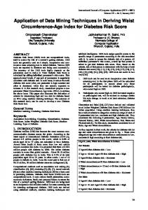
4.3.1 Software Components for the Execution Rounds An application was developed using the Java language to automate the execution rounds of the internal cycle. In order to store integrated data and results of each execution, this application was integrated with a non-relational database (MongoDB, version 3.2.0) [34]. For the machine learning task, it was built a integration with Weka software, version 3.6, through its API [28]. Moreover, it was used in application an API to integrate with the statistical package R [33], needed for the Data Integration and Interpretation of Results tasks. This API, named JRI (version 0.5.0) [59], was used to load v R dynamic library in a Java Application and provides a Java API for the R functionalities. Figure 4.1 shows the components diagram of the application:

Figure 4.1: Components Diagram of the Application developed 4.3.1.1 Data Science Application The DataScienceApp was developed using the Command design pattern [60], where each command represented a step in the Data Science Lifecycle. With ob-

CHAPTER 4.

EXPERIMENT

33

jects implemented using this pattern, it is easier to queue commands, execute and undo actions, besides other manipulations, such as delegation and sequence. These properties made possible that the Java classes were developed in way that could been executed together or separately, depending on the objective of each scenario. The reason is that in some rounds of the experiment, only a few steps needed to be performed again, such as the Command related to the Data Modelling Task. This ensured flexibility in the execution of lifecycle steps. Source code are available in a public Git repository at https://github.com/professorxavier/datascienceapp. In addition to the Command classes, the application contains classes for integration with R package, MongoDB database and Weka API. 4.3.1.2 Dataset Files The files in CSV format extracted from INMET database contained, in addition to monthly measurements, station data such as latitude, longitude and altitude. These data were important to estimate evapotranspiration using the PenmanMonteith method and were used in subsequent analyses. These files were obtained from INMET through its public Database of Meteorological Data for Education and Research [42] and comprise meteorological measures since 1961 for 263 weather stations in Brazil. Each CSV file was loaded in Java application in order to separate the station information and data series. After this loading, it was generated a new file with monthly data series (without the header) and the station data, such as latitude and longitude, extracted for storing in database. 4.3.1.3 MongoDB MongoDB [34] is one of the most popular NoSQL databases and it was used in this experiment mainly to ensure scalability for future applications. With records organized in collections of JSON documents (JavaScript Object Notation) format, data can also be read by a number of applications due to the increasing use of this format for data analysis applications. For the purpose of this research, four collections were created in MongoDB, illustrated in Figure 4.2: • Stations : to store data about each station (station name, latitude, longitude,

CHAPTER 4.

EXPERIMENT

34

altitude) • Datasets: this collection contains the imported historical measurements from CSV files as well as the value of evapotranspiration estimated by using the Penman-Monteith method. • MissingStats: this collection contains the missing data statistics for each dataset attribute of each station. • Results: for each execution, the results were stored in documents (format to store data used by MongoDB) in this collection. It was mainly used in the Interpretation of Results task of the internal cycle of Data Science and to generate reports with the experiment results.

Figure 4.2: MongoDB collections 4.3.1.4 R Package The statistical package R [33] is widely used by statisticians due to the large set of included features (organized in packages) that enable different types of analysis on datasets, from varying data sources, such as CSV files and databases. In a Data Science application, the R package is very useful in statistical analysis of data, providing the researcher with a standard set of very powerful tools and enabling the import or development of new functions/packages. In this research project, the use of the R package (version 3.1.3) was justified by its ease in extracting statistics from

CHAPTER 4.

EXPERIMENT

35

the CSV files from the INMET and the possibility of creating support functions, for specific analysis. Moreover, the R packages can be accessed by a Java program, a benefit provided by an API for integrating both technologies. In addition, the R package was crucial to estimate the values of evapotranspiration by Penman-Monteith method, due to the fact that there is a package ready to make this estimate from a data set. FAO provides a tool for this estimate but the same does not allow integration for batch execution. With the function existing in SPEI package [32] [31], described in Section 4.4.3, it was possible to estimate evapotranspiration for the entire selected dataset with a simple command, illustrated below: penman ( x$TempMinimaMedia , x$TempMaximaMedia , x$ VelocidadeVentoMedia , NA, l a t i t u d e , NA, x$ I n s o l a c a o T o t a l / 3 0 , x$ NebulosidadeMedia ,NA,NA, x$ UmidadeRelativaMedia ,NA,NA, a l t i t u d e ) In order to use this function of the SPEI package in an automated way, a function was created to process the dataset and filter it through the parameters received, in this case the years interval and the station name. Thus, it was possible to estimate evapotranspiration by the PM method for the datasets of all stations using a few lines of code and in a quick way. Below, it is shown the code of this function: pm = 5×Pthreshold and MAT >= 18 • Arid Desert Hot (BWh): MAP < 10×Pthreshold and MAP < 5×Pthreshold and MAT >= 18 • Temperate Without Dry Season and Hot Summer (Cfa): Thot >= 10 & 0 < Tcold < 18 and Not (Cs) or (Cw) and Thot >= 22 • Temperate Withoud Dry Season and Warm Summer (Cfb): Thot >= 10 & 0 < Tcold < 18 and and Not (Cs) or (Cw )and Not (a) & Tmon10 >= 4 • Temperate With Dry Winter and Hot Summer (Cwa): Thot >= 10 & 0 < Tcold < 18 and and Pwdry < Pswet/10 and Thot >= 22 • Temperate With Dry Winter and Warm Summer (Cwb): Thot >= 10 & 0 < Tcold < 18 and Pwdry < Pswet/10 and Not (a) & Tmon10 >= 4 Where:

CHAPTER 5.

RESULTS ANALYSIS

Figure 5.3: Errors points in Climate Layers for Scenario 3 • MAP = mean annual precipitation (in mm) • MAT = mean annual temperature (in °C) • Thot = temperature of the hottest month (in °C) • Tcold = temperature of the coldest month (in °C) • Tmon10 = number of months where the temperature is above 10 (units) • Pdry = precipitation of the driest month (in mm) • Psdry = precipitation of the driest month in summer (in mm) • Pwdry = precipitation of the driest month in winter (in mm) • Pswet = precipitation of the wettest month in summer (in mm) • Pwwet = precipitation of the wettest month in winter (in mm)

52

CHAPTER 5.

RESULTS ANALYSIS

53

Figure 5.4: Errors points in Climate Layers for Scenario 4 • Pthreshold = varies according to the following rules (if 70% of MAP occurs in winter then Pthreshold = 2 x MAT, if 70% of MAP occurs in summer then Pthreshold = 2 x MAT + 28, otherwise Pthreshold = 2 x MAT + 14). Summer (winter) is defined as the warmer (cooler) six month period of ONDJFM and AMJJAS (in mm) . Scenarios 2 and 4, shown in Figures 5.2 and 5.4, presented differences in some climate types in relation to Scenario 1, shown in Figure 5.1. In Scenario 2, with the inclusion of the Sunshine Hours attribute, there was an improvement in some points for the Cfa climate type, which is characterized as Temperate without Dry Season and Hot Summer. In the same Scenario, for the Aw climate type, there was an decrease in error on many points in central region and decrease on some points and northeast region. This climate type is characterized as having average temperature higher than 18 °C during the whole year and, typically, a dry season. When comparing Scenarios 1 and 4, the same behaviour was observed for the Cfa climate type, with improvements in some points, and an undefined behavior

CHAPTER 5.

RESULTS ANALYSIS

54

for the Aw climate type, with improvements in some points and error increasing in other points. In other climate types, no significant differences were observed with the inclusion of the referred attributes in the three scenarios. Additionally, it was requested maps with evapotranspiration average for each scenario, as shown in Figures 5.5, 5.6, 5.7 and 5.8.

Figure 5.5: Evapotranspiration average for Scenario 1 5.2.3 Biomes Map A biome can be defined as a regional biotic community characterized by the dominant forms of plant life and the predominant climate. There are six biomes in Brazil [43]: • The Amazon: it is the largest biome in Brazil, with a wide vegetation of about 2,500 species of trees (1/3 of all tropical wood in the world) and 30,000 plant species, representing 30% of the species in South America. • Cerrado: it is the second largest biome in South America, with headwaters of three major river basins in South America, resulting in a high potential

CHAPTER 5.

RESULTS ANALYSIS

55

Figure 5.6: Evapotranspiration average for Scenario 2 aquifer. • Pantanal: Despite being the Brazilian biome with the smallest land area, Pantanal is one of the largest continuous humid extensions of the planet. • Caatinga: it occupies about 11% of the Brazilian territory, where aproximately 27 million people live. About 80% of its original ecosystems have been changed, mainly through deforestation and fires. • Atlantic Forest: it is formed by a set of forest formations and associated ecosystems such as salt marshes, mangroves and high fields. The native vegetation is reduced to about 22% of its original size, containing about 20,000 plant species. • Pampa: The Natural Pampa landscapes are characterized by the predominance of native fields, but there is also the presence of other types of forests, riparian forests, and slope forests, among others.

CHAPTER 5.

RESULTS ANALYSIS

56

Figure 5.7: Evapotranspiration average for Scenario 3 Aiming to identify possible relationships between the results and the biomes, a second map was made using layers with the Brazilian biomes, provided by the Brazilian Institute of Geography and Statistics (IBGE) [38]. These layers were obtained in April/2016, through files in GeoJSON format available in the Brazilian Portal Open Data [40], a Brazilian platform that provides access to data from many areas. The maps with the intersection between error points and biomes layers for each scenario are shown in Figures 5.9, 5.10, 5.11 e 5.12. As well as the Climate Maps, the points represent the RRMSE values obtained in each scenario. Through an analysis made together with the domain expert on the four maps of all scenarios, some significant differences were observed in relation to the biomes. Between Scenarios 1 and 2, there were many points with better results in four biomes: Cerrado, Pantanal, Atlantic Forest and Pampa. However, in Caatinga biome, there were many points with worst results. in Amazon Biome, worst results were found on some points.

CHAPTER 5.

RESULTS ANALYSIS

57

Figure 5.8: Evapotranspiration average for Scenario 4 Comparing with Scenario 3, there were more points with worst results than points with better ones, with no significant regional patterns, occurring the same in comparison between Scenarios 1 and 4 . The differences in errors between scenarios, discussed previously in Section 5.2.2, are an evidence of a tight relationship with climate types more than biomes characteristics.

5.3 Create Actions Based in Results 5.3.1 Objectives The main objective of this phase is, after analyzing the results, to decide if more executions are required or if the results reached the objectives defined in the Problem Understanding phase. Together with the outcomes of the Visualization of Results phase, new summarized reports were provided so as to compare the results with the

CHAPTER 5.

RESULTS ANALYSIS

58

Figure 5.9: Errors points in Biomas Layers for Scenario 1 quality measures indicated in Section 3.4 and new quality measures required during the execution rounds. 5.3.2 Correlation Coefficient Results According to the evaluation proposed in Section 3.4, the correlation coefficients found were analyzed according to Table 3.2. It was established that acceptable results for this coefficient must be classified as “Very Strong Positive” at least; in other words, the coefficients must be higher than 0.70. Table 5.1: Number of Stations with Correlation Coefficients classified according to Table 3.2 Classification Very Strong Positive Moderate Positive Weak Positive

Scenario 1 101 3 1

Scenario 2 101 2 2

Scenario 3 101 3 1

Scenario 4 99 6 0

CHAPTER 5.

RESULTS ANALYSIS

59

Figure 5.10: Errors points in Biomas Layers for Scenario 2 In all scenarios and in most stations, the objective was reached, with only a small difference in Scenario 4. This scenario also had the greater number of stations with “Moderate Positive” classification. Regarding the “Weak Positive” classification, Scenarios 2 and 4 had no station. Like other graphics, this table showed that there were no major gains among the scenarios. The similar number of stations with correlation coefficients classified as ”Very Strong Positive” show that, for the correlation, the scenario with the minimum set of attributes (Scenario 1) would be sufficient to estimate evapotranspiration with good precision. 5.3.3 Relative Errors Results It was established by the domain expert that the values of Mean Absolute Error or Root Mean Square Error would be acceptable if the percentage of them in relation to the evapotranspiration average of the station were not higher than 10%, as de-

CHAPTER 5.

RESULTS ANALYSIS

60

Figure 5.11: Errors points in Biomas Layers for Scenario 3 tailed in Section 4.5.2.2. These measures, called RMAE and RRMSE, respectively, are summarized in Tables 5.2 and 5.3. Table 5.2: Number of Stations with RMAE RMAE Less than 10% Greater Than 10%

Scenario 1 96 9

Scenario 2 99 6

Scenario 3 96 9

Scenario 4 99 6

Scenarios 2 and 4 had better results than other, occurring the same with RRMSE quality measure.

5.4 Feedback out of Actions After analyzing the results and with the positive outcomes described in the previous section, we concluded that the experiment reached the initial objectives, after the domain expert evaluation.

CHAPTER 5.

RESULTS ANALYSIS

61

Figure 5.12: Errors points in Biomas Layers for Scenario 4 Table 5.3: Number of Stations with RRMSE RRMSE Less than 10% Greater Than 10%

Scenario 1 85 20

Scenario 2 87 18

Scenario 3 82 23

Scenario 4 87 18

The models generated in this research work required less attributes than PM equation, as described in Table A.1, simplifying the evapotranspiration estimation process. The PM equation requires nine attributes while models generated in this research work, illustrated in Table A.1, has five or six attributes, depending on location and shown in Table 5.4. Regarding to precision, the results had acceptable outcomes, according to results shown in Section 5.3 and the quality metrics detailed in Section 3.4. Therefore, a report was required by the domain expert with the results reached in the Second Round of Execution, detailing:

CHAPTER 5.

RESULTS ANALYSIS

62

Table 5.4: Comparison of Required Variables PM Method Wind speed Net radiation at the crop surface Soil heat flux density Mean daily air temperature Saturation vapour pressure Actual vapour pressure Saturation vapour pressure deficit Slope vapour pressure curve Psychrometric constant

Data Science Approach Wind speed Nebulosity Average Max Temperature Average Min Temperature Average Total Precipitation Total Insolation

• Station • Correlation Coefficient • MAE • RMSE • RMAE • RRMSE • Generated Equations This report was produced using the Reporting Command, illustrated in Figure 4.1, from the software developed for the experiment execution and is shown in Table A.1.

6. Related Works

6.1 Evapotranspiration In relation to evapotranspiration, there are several studies about Data Mining application for discovering alternative methods to estimate evapotranspiration. Aiming to reach an efficient irrigation management and water resources planning, Holman et al [45] proposed the use of Gaussian processes, a supervised learning model, to estimate the daily crop evapotranspiration (ET). Initially, they evaluated the data sources, analyzed some aspects of data sources such as continuity of series and availability of parameters. To select the best model, between the estimated reference ET and actual value, the root mean square error (RMSE) was used and by comparing with results obtained with linear regression (LR) models, they obtained more accuracy using the Gaussian process models. For Shiri et al [47], commonly, many data mining applications consider only a single data set assignment, as well as models are trained and tested using data of the same station. An important limitation of this approach is that the generalization of the developed models could not evaluated outside the training station. To solve this problem, their work evaluates the performance of Gene Expression Programming based models for estimating reference evapotranspiration according to temporal and spatial criteria in some locations in Iran. Results shown that in some locations, the locally trained models obtained better results that externally ones. In contrast, in other locations, externally trained models obtained better results. They concluded that externally trained models might be a valid alternative to locally trained ones, specially if there are not sufficient available local data for training a model. Regarding to required data limitation from the Penman-Monteith equation, ElShafie et al [48] proposed a modification for the Multi LayerPeceptron-Artificial 63

CHAPTER 6.

RELATED WORKS

64

Neural Network (MLP-ANN) modelling, named Ensemble Neural Network (ENN), and applied for predicting daily potential evapotranspiration. This model was applied in two regions with different climatic conditions and used data from 1975 to 2005 of only three parameters as input pattern: maximum and minimum daily temperature and solar radiation. Due to lack of lysimeters measures, data generate from the PM method were used as reference ETo in order to evaluate the proposed model. Results showed that this modified model outperformed the original one, with satisfactory level of accuracy. Xavier et al [49] developed grids of daily precipitation, evapotranspiration, and the five climate variables generally required to estimate evapotranspiration in Brazil, using data between 1980 and 2013, with the objective of providing a gridded meteorological data set. They used data from the National Institute of Meteorology (INMET), the National Water Agency (ANA), and the Department of Water and Power of São Paulo (DAEE) and, using some quality measures, they applied a quality control check discarding all data that failed in quality measures. To create the gridded daily data, they used an interpolation method chosen from the evaluation of six interpolation methods. Another interesting characteristic of this research was the method used to present data: a scatter diagram in the Brazilian map, providing an evaluation by region. As conclusions, they observed that performance depends on both the amount of data available and the season. Other studies refer to use remotely sensed data to estimate evapotranspiration. Li et al [54] made a review of methodologies for evapotranspiration estimation using this method for getting data. For them, the remote sensing technology has many advantages over local measurements, such as data generation for large areas in short time and it is practical for using in areas where measurements are difficult. However, for Liou and Kar [55], some methods using this technology have low accuracy while other have limitations over mountainous areas.

6.2 Data Science Due to its multidisciplinary nature, the application of the Data Science techniques is a subject of several scientific papers in different areas of knowledge, such as Climate Changes, Agriculture, Health, Business Process Management, etc. Regarding Hydrology, many research work consisted of reports of experiences of the application of data mining, with several objectives. In Hewett research [44],

CHAPTER 6.

RELATED WORKS

65

data mining was used to generate predictive models of future water inflows of a lake in Florida. The author applied table compression induction and results were compared with three data analyses techniques: neural networks, decision tree and associational rule mining. The table compression induction aims to solve the problem with large tables, transforming the original table in a table with fewer and more general rules. This technique produced a lower error rate than other data mining techniques compared. Another work using data mining was produced by Keskin et al [46], that used data mining for evaporation estimation, using daily pan evaporation data of three lakes in Turkey. REP tree, KStar, decision table, artificial neural networks and multilinear regression were the algorithms used in the research, with the best results obtained with REP tree. For Zanin [50], Data Science may provide insights in analysis of historical data sets that cannot be easily discovered just by manual analysis or by relying on expert judgement. His research used Data Science techniques to improve the analysis of historical data in air transport and ATM, limited by the difficulties inherent to study of heterogeneous data sets. In the conclusions, he pointed out an important aspect of Data Science application in order to solve common problems: ’listen to the data’. Shcherbakov et al [9] proposed a Lean Data Science Lifecycle with study case made for energy time series analysis. They used Python scripts for Task Statement and Data Integration tasks and used a chart for the Visualization of Results phase of proposed lifecycle. Regarding to the transportation systems, Lin [51] proposed an integrated approach for data science applications in intelligent transportation systems (ITS). This approach comprises the integration of multiple steps in the data analysis process or the integration of different models to build a more powerful one. For evaluation, two case studies were made: to border crossing delay prediction and traffic accident data analysis. To create an integrated database, multiple data sources were used such as fixed sensors data, connected vehicles data, traffic accident data, social media data. Some algorithms were used to analyze data and to create a forecasting model, such as MP5 tree.

CHAPTER 6.

RELATED WORKS

66

6.3 Summary The study of related works shown that there is extensive research using computer techniques in evapotranspiration subject and some aspects can be highlighted from these researches. The first one regards to the objective of simplifying the currently methods to estimate evapotranspiration. Although many works are only experience reports of data mining processes, it is clear that data-driven approaches may be an alternative for the currently methods used. The studies presented in this section showed a diverse use of techniques to propose new methods for evapotranspiration estimation, such as Gaussian processes and neural networks. It was also observed the form to present the results, such as in Xavier et al research [49], with the use of maps to view the results. A second aspect is related to comparison methods. Despite of the PM model limitations, this method is normally used to compare results of the alternative methods. This fact is due to absence of real measures of evapotranspiration and because PM model is the reference from the FAO. Related to the Data Science techniques application, there are some experience reports in different domains. Many of these reports have described data mining application, which is only one technique of the Data Science set. Some researches were based in proposed lifecycle for Data Science application, such as the research conducted by Shcherbakov et al [9]. In Lin research [51], many techniques from Data Science were used, comprising from data integration to visualization of results. This research seems to be the closest one to a complete Data Science application, using the key differentiator defined by Loukides [22]: a holistic approach with data and not only the use of some techniques. This approach is the main difference from this research project in relation to the related works presented in this Chapter. These works were focused in simplify the evapotranspiration estimation but using only one specific technique, such as data mining or interpolation. By other side, this research work was applied on phases of data lifecycle and had deeply interaction with the domain expert, in all step of the Data Science lifecycle. In addiction, the approach presented in this research was focused in product delivery for end users and providing the repeatability characteristic of experiment.

7. Conclusions

7.1 Final Considerations This research project applied techniques from Data Science to solve a known problem in the Hydrology domain: the estimation of evapotranspiration, a critical component in the water cycle. Currently, there are many methods to estimate evapotranspiration, such as the Penman-Monteith and Thornthwaite models. The former is considered to be the most precise model and is recommended by FAO. However, it is described in the literature as a very complex model, requiring many variables, which restricts its use in regions that do not have measurements for all required variables. The second model, used by INMET, is simpler when compared to the Penman-Monteith model, but it underestimates evapotranspiration under dry conditions. Despite of the advantages and disadvantages of both models, they share one common characteristic: since the evapotranspiration process using these approaches is model-driven, the measurement of the required variables is mandatory. In the absence of values of any variable, their application are not possible. One recommendation for the missing data problem is to use values from near locations. Although it partially solves the missing data problem, this approach has a cost on precision. Based on the limitations in current models, the persent work addressed the following research question: Is it possible to simplify evapotranspiration estimation with good precision? Considering the above, this research proposed a new approach to estimate evapotranspiration values, based on a key difference from current models: the estimation is data-driven. In other words, our evapotranspiration estimation models are built from the data gathered at the measurement stations. 67

CHAPTER 7.

CONCLUSIONS

68

In order to accomplish this goal, Data Science techniques were used. They offer a new way to extract value from data, generating products to solve research questions. There are other techniques to work with data, some of them included in the set of Data Science tools and methods. However, the key characteristic of Data Science is its holistic approach to working with data, with the application of its techniques on the whole data cycle. Another important change brought by Data Science is the high level of engagement of domain experts in the research process. Data Science can be applied for all knowledge areas, but it is not required that data scientists have deep knowledge about many domains. Therefore, the domain expert is a fundamental component in the Data Science lifecycle, participating from the problem definition step to the evaluation of results. Although data scientists could bring insights and propose new strategies, the domain expert is the one who has enough knowledge to validate results and propose solutions. For this research, a hydrology expert has taken the role of domain expert, proposing research questions, discussing strategies, suggesting new experiment scenarios and validating the outcomes. In the application of Data Science in this research, we adopted a Data Science lifecycle based on Lean Development. This lifecycle was used for its high level of interaction and fast delivery of results to be evaluated by the domain expert. In the internal cycle of the adopted Data Science lifecycle, two rounds of execution were needed, with adjusts suggested by the domain expert. After the execution of the second round and the interpretation of the results, it was required by the domain expert that results be summarized in graphs and plotted in maps. The objective of this phase was to check whether the results had a positive outcome and identify possible relationships with the results and regional characteristics. After analyzing the results, the domain expert concluded that these results presented a positive outcome, reaching the goals defined in the solution evaluation section and the new quality measures defined during the internal cycle. With the models generated in this approach for evapotranspiration estimation, it was possible to simplify the estimation process, requiring less variables than PenmanMonteith model, decreasing from nine required variables to five or six, depending on model generated for each measurement station used in this research, as shown in Table 5.4. Regarding to the quality metrics for precision, defined in the Subsec-

CHAPTER 7.

CONCLUSIONS

69

tion 4.5.2.2, this research it was successfull for the most stations used in experiment steps, as shown in Tables 5.2 and 5.3. Thus, it was possible to conclude that this research reached its objective with positive outcomes, according to the goals defined in previous Chapters.

7.2 Contributions This research contributed to both areas of Information Systems and Hydrology. For Information Systems research, the Data Science application using a lifecycle based on the Lean Development showed the importance of the domain expert in a Data Science research project as well the need for fast deliveries so as to guarantee the high level of interaction with the domain expert. Regarding the artifacts and methods used, this research showed how Data Science is more than a data analysis method. In order to provide the results required by the domain expert, many tools and technologies were needed and they were integrated by a developed software. This research used programming languages such as Java and R, a data mining tool (Weka), a non-relational database (MongoDB), and tools for results visualization in georeferenced forms. Basic statistics analysis was also used to generate information about the datasets in preliminary phases of the Data Science lifecycle as well as in the intermediary and final phases, in the evaluation of results. As for areas related to water studies, such as Hydrology, this research contributed with a new approach to analyze meteorological data for the estimation of evapotranspiration. Furthermore, the results plotted in maps with climate and biomes layers provided a view of this approach in relation to regional characteristics, such as climate and vegetation. Besides, these maps could be used for new experiments in other topics or even in the subject of evapotranspiration. The simplified models for evapotranspiration estimation could also be considered a contribution of this work. Researchers would be able to use these models to estimate evapotranspiration as well as to compare them with other methods.

CHAPTER 7.

CONCLUSIONS

70

7.3 Future Work Many works could originate from this research. An extension of this work, using more measurement stations and increasing the number of instances, could produce more information about evapotranspiration estimation. Also, a deeper study could be made about the relationships of the local characteristics, such as climate and vegetation. Other environmental aspects, such as soil types, could also be the subject of new studies. The soil type has an important relation with the evapotranspiration rate, depending on the soil’s water absorption capacity. In this study, a minimum set of attributes for evapotranspiration estimation was used with the inclusion of two other attributes: total precipitation and sunshine hours. Other studies could be made using other climatic and meteorological attributes and evaluating the impact of the inclusion of these attributes. This research had, as initial objective, a less number possible of variables used in the evapotranspiration estimation. However, new studies can be made using all variables presents in meteorological datasets, that could show which variables are more important in the evapotranspiration estimation. The algorithm used for the Data Modelling task was M5P, as shown in 4.4.5. New studies could be made with other algorithms, comparing them and evaluating which algorithm would be better for a defined conditions set, such as variables available or physical local conditions. The approach used here could also be used to fill the missing data in the data historical series, increasing the range of periods for further studies. Another suggestion could be the use of the Data Science approach applied here to study the possible errors in the data historical series. Regarding Data Science studies, the lifecycle adopted here could be object of study with proposals of changes and studying the impact of these changes in the results. In this suggestion, the main object of study could be the own process of Data Science application, proposing alternatives lifecycles, identifying better practices for the lifecycle tasks, etc. Finally, the approach used here could be used in other knowledge areas, such as biodiversity or health. These areas have many data from different sources that could be used in some research projects.

Bibliography

[1] Allen, Richard G., Pereira, Luis S., Raes, Dirk, Smith, Martin, 1998, ”Crop evapotranspiration-Guidelines for computing crop water requirements-FAO Irrigation and drainage paper 56.”, FAO, Rome, 1998. [2] Cleveland, William S, 2001, ”Data science: an action plan for expanding the technical areas of the field of statistics”, International statistical review, v. 69, number 1, pp. 21-26, Wiley Online Library, 2001. [3] Conway, Drew, 2013, ”The Data Science Venn Diagram”, Drew Conway Website, Available in: http://drewconway.com/zia/2013/3/26/the-data-sciencevenn-diagram, 2013. [4] Evans, John, Perlman, Howard, 2015, ”The Water Cycle”, U. S. Geological Survey, Available in: http://water.usgs.gov/edu/watercycle.html. [5] Fahle, Marcus and Dietrich, Ottfried, 2014, ”Estimation of evapotranspiration using diurnal groundwater level fluctuations: Comparison of different approaches with groundwater lysimeter data”, Water Resources Research, v. 50, number 1, pp. 273-286, Wiley Online Library, 2014. [6] Fernandes, Antônio Vitor Barbosa, 2015, ”Evapotranspiração e sua Influência na Engenharia Civil”, Caderno de Graduação-Ciências Exatas e TecnológicasUNIT, v. 2, Issue 3, pp. 21-36, 2015. [7] Kumar, R and Jat, MK and Shankar, V, 2012, ”Methods to estimate irrigated reference crop evapotranspiration a review”, Water Science and Technology, v. 66, number 3, pp. 525-536. [8] Penman, Howard Latimer, 1948, ”Natural evaporation from open water, bare soil and grass”, Proceedings of the Royal Society of London A: Mathematical, Physical and Engineering Sciences, v. 193, number 1032, pp. 120-145. 71

BIBLIOGRAPHY

72

[9] Shcherbakov, Maxim, Shcherbakova, Nataliya, Brebels, Adriaan, Janovsky, Timur, Kamaev, Valery, 2014, ”Lean Data Science Research Life Cycle: A Concept for Data Analysis Software Development”, Knowledge-Based Software Engineering, v. 466, pp. 708-716, Springer International Publishing, 2014. [10] Thornthwaite, Charles Warren, 1948, ”An approach toward a rational classification of climate”, Geographical review, v. 38, Issue 1, pp 45-94, Jan. 1948. [11] Vera-Repullo, JA and Ruiz-Peñalver, L and Jiménez-Buendía, M and Rosillo, JJ and Molina-Martínez, JM, 2015, ”Software for the automatic control of irrigation using weighing-drainage lysimeters”, Agricultural Water Management, v. 151, pp. 4-12, Elsevier, 2015. [12] Xavier, Fernando and Tanaka, Asterio Kiyoshi and Revoredo, Kate Cerqueira, 2015, ”Application of Knowledge Discovery in Databases in Evapotranspiration Estimation: an Experiment in the State of Rio de Janeiro”, Proceedings of the annual conference on Brazilian Symposium on Information Systems: Information Systems: A Computer Socio-Technical, v. 1, pp. 25-33, Brazilian Computer Society, 2015. [13] Xavier, Fernando and Tanaka, Asterio Kiyoshi and Revoredo, Kate Cerqueira, 2015, ”Aplicaç ao de KDD em Dados Meteorológicos para Identificaç ao de Padroes Regionais na Estimativa da Evapotranspiraç ao”, Proceedings of Satellite Events of the 30th Brazilian Symposium on Databases, Brazilian Computer Society, 2015. v. 1. p. 27-32. [14] Majidi, M. and Alizadeh, A. and Vazifedoust, M. and Farid, A. and Ahmadi, T., 2015, ”Analysis of the Effect of Missing Weather Data on Estimating Daily Reference Evapotranspiration Under Different Climatic Conditions”, Water Resources Management, v. 29, Issue 7, pp. 2107-2124, Springer Netherlands. [15] Liou, Yuei-An and Kar, Sanjib Kumar, 2014, ”Evapotranspiration estimation with remote sensing and various surface energy balance algorithms—A review”, Energies, v. 7, Issue 5, pp. 2821-2849, Multidisciplinary Digital Publishing Institute. [16] Mueller, Lothar and Saparov, Abdulla and Lischeid, Gunnar, 2014, ”A Field Method for Quantifying Deep Seepage and Solute Leaching”, Novel Measurement and Assessment Tools for Monitoring and Management of Land and Water Resources in Agricultural Landscapes of Central Asia, pp. 185-198.

BIBLIOGRAPHY

73

[17] Camargo, A.P. de and Marin, F.R. and Sentelhas, P. C. and Picini, A.G., 1999, ”Ajuste da equação de Thornthwaite para estimar a evapotranspiração potencial em climas áridos e superúmidos, com base na amplitude térmica diária”, Revista Brasileira de Agrometeorologia, v. 7, Issue 2, pp. 251-257 [18] van der Aalst, Wil MP, 2014, ”Data scientist: The engineer of the future”, Enterprise Interoperability VI, pp. 13-26, Springer [19] Zhu, Yangyong and Zhong, Ning and Xiong, Yun, 2009, ”Data explosion, data nature and dataology”, Brain Informatics, pp. 147-158, Springer [20] Margolis, Ronald and Derr, Leslie and Dunn, Michelle and Huerta, Michael and Larkin, Jennie and Sheehan, Jerry and Guyer, Mark and Green, Eric D, 2014, ”The National Institutes of Health’s Big Data to Knowledge (BD2K) initiative: capitalizing on biomedical big data”, Journal of the American Medical Informatics Association, v. 21, issue 6, pp. 957-958, The Oxford University Press [21] Chauhan, Seema and Shrivastava, RK, 2009, ”Performance evaluation of reference evapotranspiration estimation using climate based methods and artificial neural networks”, Water resources management, v. 23, issue 5, pp. 825-837, Springer [22] Loukides, Mike, 2010, ”What is data science”, O’Reilly Website - Ideas, Available in: http://radar.oreilly.com/2010/06/what-is-data-science.html. [23] Barros, Vinicius Rios and de Souza, Adilson Pacheco and Fonseca, Daniel Carvalho and da Silva, Leonardo Batista Duarte, 2009, ”Avaliação da evapotranspiração de referência na região de Seropédica-RJ, utilizando lisímetro de pesagem e modelos matemáticos”, Brazilian Journal of Agricultural Sciences, v. 4, issue 2, pp. 198–203 [24] de Camargo, Ângelo Paes and de Camargo, Marcelo Bento Paes, 2000, ”Uma revisão analítica da evapotranspiração potencial”, Bragantia, v. 59, issue 2, pp. 125–137 [25] de Souza, Alexandre da Silva Pinheiro, 2011, ”Evaluation of Methods for Estimation Reference evapotranspiration for Irrigation Water Management”, PhD dissertation, Federal University of Rio de Janeiro

BIBLIOGRAPHY

74

[26] Lee Rodgers, Joseph and Nicewander, W Alan, 1988, ”Thirteen ways to look at the correlation coefficient”,The American Statistician, v. 42, issue 1, pp. 59–66 [27] Viaene, Stijn, 2013, ”Data Scientists Aren’t Domain Experts”,IT Professional, number 6, pp. 12–17, IEEE [28] Hall, Mark, Frank, Eibe, Holmes, Geoffrey, Pfahringer, Bernhard, Reutemann, Peter and Witten, Ian H , 2009, ”The WEKA Data Mining Software: An Update”,SIGKDD Explorations, v. 11, issue 1 [29] Wang, Y., & Witten, I. H., 1996, ”Induction of model trees for predicting continuous classes”,Poster papers of the 9th European Conference on Machine Learning, Springer, 1997 [30] Quinlan, Ross J., 1992, ”Learning with Continuous Classes”,In: 5th Australian Joint Conference on Artificial Intelligence, Singapore, pp. 343-348, 1992. [31] Beguería, Santiago and Vicente-Serrano, Sergio M and Reig, Fergus and Latorre, Borja , 2014, ”Standardized precipitation evapotranspiration index (SPEI) revisited: parameter fitting, evapotranspiration models, tools, datasets and drought monitoring”,International Journal of Climatology, v. 34, number 10, pp. 3001-3023 [32] Beguería, Santiago and Vicente-Serrano, Sergio M, 2013, ”SPEI: Calculation of the Standardised Precipitation-Evapotranspiration Index”, Standardized Precipitation-Evapotranspiration Index, Available in: https://cran.rproject.org/web/packages/SPEI/index.html. [33] R Core Team, 2013, ”R: A Language and Environment for Statistical Computing”, R Foundation for Statistical Computing, Available in: http://www.Rproject.org. [34] MongoDB

Inc.,

2016,

”MongoDB”,

MongoDB,

Available

in:

https://www.mongodb.com. [35] QGIS Development Team, 2009, ”QGIS Geographic Information System”, Open Source Geospatial Foundation, Available in: http://qgis.osgeo.org. [36] Agafonkin, Vladimir, 2016, ”Leaflet - an open-source JavaScript library for mobile-friendly interactive maps”, Leaflet, Available in: http://leafletjs.com/.

BIBLIOGRAPHY

75

[37] Melo, Giovani L de and Fernandes, André LT, 2012, ”Evaluation of empirical methods to estimate reference evapotranspiration in Uberaba, State of Minas Gerais, Brazil”, Engenharia Agrícola, v. 32, Issue 5, pp. 875-888, SciELO Brasil. [38] IBGE, 2016, ”Biomas do Brasil”, Instituto Brasileiro de Geografia e Estatística, Available in: http://www.geoservicos.ibge.gov.br/. [39] Peel MC, Finlayson BL, McMahon TA, 2007, ”Updated world map of the Köppen-Geiger climate classification”, Hydrol. Earth Syst. Sci., 11, 1633-1644. [40] Brazilian Open Data Portal, 2016, ”Mapa Temático - Biomas do Brasil”, Portal Brasileiro de Dados Abertos, Available in: http://tinyurl.com/h8h35b6. [41] INMET, 2016, ”National Institute of Meteorology”, Ministry of Agriculture, Livestock and Supply - Brazilian Government, Available in: http://www.inmet.gov.br. [42] BDMEP, 2016, ”BDMEP - Database of Meteorological Data for Education and Research”, National Institute of Meteorology, Available in: http://www.inmet.gov.br/projetos/rede/pesquisa/. [43] MMA, 2016, ”Biomes”, Ministry of the Environment - Brazilian government, Available in: http://www.mma.gov.br/biomas/. [44] Hewett, Rattikorn, 2003, ”Data mining for generating predictive models of local hydrology”, Applied Intelligence, v. 19, issue 3, pp. 157-170. [45] Holman, Daniel and Sridharan, Mohan and Gowda, Prasanna and Porter, Dana and Marek, Thomas and Howell, Terry and Moorhead, Jerry, 2014, ”Gaussian process models for reference ET estimation from alternative meteorological data sources”, Journal of Hydrology, v. 517, pp. 28-35. [46] Keskin, M Erol and Terzi, Özlem and Küçüksille, E Uğur, 2009, ”Data mining process for integrated evaporation model”, Journal of Irrigation and Drainage Engineering, v. 135, issue 1, pp. 39-43. [47] Shiri, Jalal and Sadraddini, Ali Ashraf and Nazemi, Amir Hossein and Kisi, Ozgur and Landeras, Gorka and Fakheri Fard, Ahmad and Marti, Pau, 2014, ”Generalizability of Gene Expression Programming-based approaches for estimating daily reference evapotranspiration in coastal stations of Iran”, Journal of Hydrology, v. 508, pp. 1-11.

BIBLIOGRAPHY

76

[48] El-Shafie, Ahmed and Najah, Ali and Alsulami, Humod Mosad and Jahanbani, Heerbod, 2014, ”Optimized neural network prediction model for potential evapotranspiration utilizing ensemble procedure”, Water Resources Management, v. 28, issue 4, pp. 947-967. [49] Xavier, Alexandre C. and King, Carey W. and Scanlon, Bridget R., 2016, ”Daily gridded meteorological variables in Brazil (1980–2013)”, International Journal of Climatology, v. 36, pp.2644–2659. [50] Zanin, Massimiliano, 2013, ”The reasonable effectiveness of data in ATM”, Third SESAR Innovation Days. [51] Lin, Lei, 2015, ”Data science application in intelligent transportation systems: An integrative approach for border delay prediction and traffic accident analysis”, Doctoral dissertation, State University of New York at Buffalo. [52] Overpeck, J. T., Meehl, G. A., Bony, S., & Easterling, D. R., 2011, ”Climate data challenges in the 21 st century”, Science, v. 331, issue 6018, pp. 700-702. [53] Mattmann, C. A., 2013, ”Computing: A vision for data science”, Nature, issue 493, pp. 473-475. [54] Li, Zhao-Liang and Tang, Ronglin and Wan, Zhengming and Bi, Yuyun and Zhou, Chenghu and Tang, Bohui and Yan, Guangjian and Zhang, Xiaoyu, 2009, ”A review of current methodologies for regional evapotranspiration estimation from remotely sensed data”, Sensors, v. 9, issue 5, pp. 3801-3853. [55] Liou, Yuei-An and Kar, Sanjib Kuma, 2014, ”Evapotranspiration estimation with remote sensing and various surface energy balance algorithms—A review”, Sensors, v. 7, issue 5, pp. 2821-2849. [56] Di Bello, R. C., 2005, ”Análise do Comportamento da Umidade do Solo no Modelo ChuvaVazão Smap II–Versão com Suavização Hiperbólica Estudo de Caso: Região de Barreiras na Bacia do Rio Grande-BA”,Master dissertation, Federal University of Rio de Janeiro. [57] Ballé, Freddy and Ballé, Michael, 2005, ”Lean development”, Business Strategy Review, v. 16, issue 3, pp. 17-22. [58] Chai, Tianfeng and Draxler, Roland R, 2014, ”Root mean square error (RMSE) or mean absolute error (MAE)?–Arguments against avoiding RMSE in the literature”, Geoscientific Model Development, v. 7, issue 3, pp. 1247-1250.

BIBLIOGRAPHY

77

[59] RForge, 2016, ”JRI - Java/R Interface”, RForge, Available in: https://rforge.net/JRI/. [60] Gamma, E., Helm, R., Johnson, R., Vlissides, J., 1994, ”Design patterns: elements of reusable object-oriented software”, Addison-Wesley, 395 pages, ISBN 0-201-63361-2. [61] Weka Team, 2016, ”Use WEKA in your Java code”, RForge, Available in: https://weka.wikispaces.com/Use+WEKA+in+your+Java+code. [62] NTSG, 2016, ”MODIS Global Evapotranspiration Project (MOD16)”, Numerical Terradynamic Simulation Group/The University of Montana, Available in: http://www.ntsg.umt.edu/project/mod16. [63] FAO, 2016, ”CropWat”, Available in: fores_databases_cropwat.html.

http://www.fao.org/nr/water/in-

A.Detailed Results for All Stations

78

0.880516

0.773381

0.764455

0.777869

0.744311

0.694584

0.898560

0.958187

0.787464

ac_riobranco

am_coari

am_fonteboa

am_itacoatiara

am_manaus

am_parintins

ap_macapa

ba_alagoinhas

ba_bomjesus-

dalapa

0.690391

tion

Correla-

ac_cruzeirodosul

Station Name

11.88252

6.970123

4.986404

7.296429

6.764233

6.058515

6.046596

6.423996

7.221780

10.06740

MAE

13.99465

8.599386

6.497315

8.830467

8.081658

7.395250

7.384419

7.858785

9.109672

11.93523

RMSE

0.071573

0.044087

0.029817

0.045614

0.041340

0.037801

0.037910

0.039349

0.045981

0.066046

RMAE

0.084295

0.054393

0.038852

0.055204

0.049391

0.046141

0.046298

0.048138

0.058002

0.078299

RRMSE

MT - 220.9816

LM num: 1 => evp = 0.1006 * TI + 9.756 * NM + 0.081 * TP + 9.5387 *

LM num: 1 => evp = 40.5553 * WA + 7.7993 * MT - 155.6012

LM num: 1 => evp = 14.2305 * WA - 0.033 * TI + 4.7602 * MT - 6.8756

MT + 2.8377 * MiT - 82.2519

evp = 8.4111 * WA - 0.0095 * TI + 2.5769 * NM + 0.0157 * TP + 4.8861 *

TI + 2.5736 * NM + 4.3614 * MT + 0.3824 * MiT - 3.9908LM num: 3 =>

MT - 0.6045 * MiT + 17.833LM num: 2 => evp = 3.2888 * WA - 0.0064 *

LM num: 1 => evp = 3.2888 * WA - 0.0064 * TI + 4.2563 * NM + 3.9279 *

* TP + 12.9947 * MT - 262.8247

LM num: 1 => evp = 9.7355 * WA - 0.1587 * TI + 1.8461 * NM + 0.0219

* MT - 160.7222

LM num: 1 => evp = 39.2211 * WA + 5.0083 * NM + 0.0233 * TP + 7.809

LM num: 1 => evp = 9.7419 * NM + 14.263 * MT - 369.7485

NM + 0.0098 * TP + 12.0924 * MT - 283.4719

TP + 5.4842 * MT - 52.4685LM num: 3 => evp = 5.9118 * WA + 6.3825 *

* MT - 97.8831LM num: 2 => evp = 8.7229 * WA + 3.863 * NM - 0.0037 *

LM num: 1 => evp = 16.1824 * WA + 4.7045 * NM + 0.0226 * TP + 6.0739

* MT - 281.097

LM num: 1 => evp = 28.5399 * WA + 9.2182 * NM + 0.0373 * TP + 10.7059

0.0267 * TP + 3.8427 * MT + 1.0144 * MiT + 2.9716

86.0698LM num: 5 => evp = 6.9064 * WA - 0.0361 * TI + 0.9552 * NM +

- 0.0438 * TI - 0.3353 * NM + 0.0288 * TP + 5.1052 * MT + 3.479 * MiT -

+ 5.2802 * MT + 3.479 * MiT - 93.7352LM num: 4 => evp = 12.948 * WA

num: 3 => evp = 12.0649 * WA - 0.0438 * TI - 0.1202 * NM + 0.0288 * TP

TI + 0.9552 * NM + 0.0288 * TP + 7.1695 * MT + 4.7761 * MiT - 194.49LM

* MT - 0.5111 * MiT - 135.3684LM num: 2 => evp = 9.695 * WA - 0.0438 *

LM num: 1 => evp = 12.5601 * WA + 1.7313 * NM + 0.1026 * TP + 8.0377

Models

Table A.1: Execution Results for Scenario 4

APPENDIX A. DETAILED RESULTS FOR ALL STATIONS 79

0.926407

0.926505

0.952307

0.884323

0.864496

0.849791

0.778497

0.899673

0.930777

0.925790

0.911877

0.881647

0.926295

0.937545

ba_caravelas

ba_cipo

ba_feiradesantana

ba_ituacu

ce_barbalha

ce_crateus

ce_fortaleza

ce_guaramiranga

ce_iguatu

ce_jaguaruana

df_brasilia

df_roncador

go_aragarcas

go_catalao

8.076088

9.193125

8.298197

7.730520

6.911890

6.574101

5.434244

5.991667

8.562495

7.581262

9.862507

8.629320

8.361942

9.005550

10.38639

11.82595

10.78292

9.921597

8.092358

8.037068

6.909544

7.649599

10.46908

9.486599

12.34818

10.05246

11.69584

11.29342

0.052252

0.062105

0.054251

0.052061

0.036143

0.035649

0.037558

0.035820

0.044794

0.045526

0.061732

0.050863

0.046394

0.062249

0.067199

0.079891

0.070495

0.066817

0.042315

0.043582

0.047754

0.045732

0.054768

0.056968

0.077290

0.059252

0.064892

0.078063

* MT - 2.7732 * MiT - 258.4117

LM num: 1 => evp = 16.5974 * WA + 9.894 * NM + 0.038 * TP + 13.002

* NM + 0.0266 * TP + 4.0925 * MT + 2.4716 * MiT - 52.1642

* MiT - 106.7189LM num: 3 => evp = 10.9377 * WA - 0.0165 * TI + 4.2617

* WA - 0.0165 * TI + 4.5766 * NM + 0.0806 * TP + 4.9916 * MT + 2.7367

TP + 8.4923 * MT + 1.1625 * MiT - 215.2804LM num: 2 => evp = 11.8388

LM num: 1 => evp = 7.7563 * WA - 0.0248 * TI + 8.2192 * NM + 0.0227 *

* MT - 214.1632

LM num: 1 => evp = 14.4381 * WA + 6.919 * NM + 0.034 * TP + 10.7174

* MT - 213.355

LM num: 1 => evp = 12.6467 * WA + 5.3918 * NM + 0.0618 * TP + 10.933

* MiT - 62.6764

LM num: 1 => evp = 13.8823 * WA + 0.1893 * TI + 2.6729 * MT + 2.8604

* MiT - 295.8653

LM num: 1 => evp = 12.3046 * WA + 0.0398 * TP + 8.6911 * MT + 6.7259

* MiT - 193.0077

LM num: 1 => evp = 4.5187 * NM + 0.0434 * TP + 14.7655 * MT - 4.4592

* TI + 0.0228 * TP + 12.3165 * MT - 237.8026

* TP + 12.1733 * MT - 302.9193LM num: 2 => evp = 3.2996 * WA + 0.035

LM num: 1 => evp = 2.6397 * WA + 0.1754 * TI + 4.9852 * NM + 0.0447

LM num: 1 => evp = 0.0967 * TP + 12.78 * MT - 248.6993

* TP + 9.8497 * MT - 234.9181

LM num: 1 => evp = 10.0855 * WA + 0.1411 * TI + 4.7999 * NM + 0.0705

* TP + 10.3698 * MT - 312.2645

LM num: 1 => evp = 23.9634 * WA + 0.1823 * TI + 10.1044 * NM + 0.1548

* TP + 13.4312 * MT - 5.6783 * MiT - 149.643

LM num: 1 => evp = 19.4011 * WA - 0.0814 * TI - 5.7426 * NM + 0.1108

* MT - 8.1806 * MiT - 314.9227

LM num: 1 => evp = 26.6686 * WA + 5.5898 * NM + 0.1255 * TP + 17.0235

371.5959

LM num: 1 => evp = 28.6745 * WA + 5.4723 * NM + 14.6622 * MT -

APPENDIX A. DETAILED RESULTS FOR ALL STATIONS 80

0.910863

0.938229

0.946459

0.945535

0.878950

0.931125

0.847816

0.960740

go_formosa

go_goiania

go_ipameri

go_jatai

go_pirenopolis

go_posse

ma_balsas

ma_chapadinha

4.872455

6.988021

6.657817

8.803028

7.752084

8.272277

7.380511

8.106126

6.399559

8.553390

8.442997

10.81574

10.28976

10.25602

9.890492

10.90883

0.027270

0.042704

0.044322

0.053429

0.050909

0.057259

0.048193

0.055805

0.035817

0.052270

0.056206

0.065645

0.067575

0.070990

0.064583

0.075099

* TP + 11.939 * MT - 364.2609

LM num: 1 => evp = 9.6608 * WA + 0.2748 * TI + 11.8022 * NM + 0.0228

11.2012 * MT - 285.2129

LM num: 1 => evp = 31.1953 * WA + 10.2242 * NM + 0.0279 * TP +

3.0885 * NM + 0.0381 * TP + 7.2936 * MT - 2.9195 * MiT - 20.8226

* MT + 2.7699 * MiT - 236.9848LM num: 2 => evp = -4.2871 * WA +

LM num: 1 => evp = 19.5259 * WA + 2.8257 * NM + 0.0349 * TP + 9.4319

* MT - 232.804

LM num: 1 => evp = 22.4184 * WA + 6.8688 * NM + 0.098 * TP + 9.5369

1.1092 * MiT - 85.1073

=>0 evp = 14.2119 * WA + 0.2346 * TI + 10.1672 * NM + 3.6818 * MT +

* TI + 10.1857 * NM + 3.6818 * MT + 1.1092 * MiT - 86.4526LM num: 1

MT + 1.1092 * MiT - 86.4705LM num: 9 => evp = 14.7889 * WA + 0.2346

num: 8 => evp = 14.7889 * WA + 0.2346 * TI + 10.1857 * NM + 3.6818 *

+ 0.2456 * TI + 10.0572 * NM + 3.6818 * MT + 1.1092 * MiT - 87.5728LM

3.6818 * MT + 1.1092 * MiT - 70.3039LM num: 7 => evp = 14.2119 * WA

163.0864LM num: 6 => evp = 14.2119 * WA + 0.1956 * TI + 8.969 * NM +

11.9872 * WA + 0.1534 * TI + 8.5118 * NM + 6.7568 * MT + 1.1092 * MiT -

8.5118 * NM + 6.8692 * MT + 1.1092 * MiT - 181.7157LM num: 5 => evp =

1.1092 * MiT - 181.0113LM num: 4 => evp = 24.6991 * WA + 0.1534 * TI +

=> evp = 23.4637 * WA + 0.1534 * TI + 8.5118 * NM + 6.8692 * MT +

* TI + 4.0192 * NM + 5.3459 * MT + 1.743 * MiT - 122.7843LM num: 3

* MT + 1.743 * MiT - 106.1963LM num: 2 => evp = 22.5983 * WA + 0.0769

LM num: 1 => evp = 24.8943 * WA + 0.0769 * TI + 4.0192 * NM + 4.5435

* MiT - 201.6557

LM num: 1 => evp = 38.5638 * WA + 8.8475 * NM + 7.6014 * MT + 2.7112

* MT - 224.4238

LM num: 1 => evp = 51.0842 * WA + 9.0291 * NM + 0.0582 * TP + 8.3844

* MT - 193.3139

LM num: 1 => evp = 23.0851 * WA - 0.2026 * TI + 5.9085 * NM + 11.5951

APPENDIX A. DETAILED RESULTS FOR ALL STATIONS 81

0.929139

0.946260

0.952069

0.963111

0.938585

0.961650

0.482340

0.886613

0.927785

0.966296

mg_araxa

mg_arinos

mg_bambui

mg_belohorizonte

mg_caparao

mg_caratinga

mg_formoso

mg_janauba

mg_januaria

mg_lavras

6.820644

7.657949

9.227944

16.20675

7.903542

9.658303

6.752426

9.096161

7.391903

9.486400

8.960971

9.583381

11.13636

19.86183

9.566662

12.40308

8.981649

10.83707

9.635445

11.22469

0.046175

0.045005

0.055391

0.105232

0.054819

0.073704

0.047865

0.064147

0.047589

0.063140

0.060665

0.056321

0.066846

0.128965

0.066355

0.094650

0.063667

0.076424

0.062033

0.074710

* TP + 12.1619 * MT - 2.7672 * MiT - 323.5264

LM num: 1 => evp = 28.8424 * WA + 0.2104 * TI + 11.5835 * NM + 0.0636

* TP + 4.9247 * MT + 4.5769 * MiT - 299.5716

LM num: 1 => evp = 36.2143 * WA + 0.4052 * TI + 11.6934 * NM + 0.0767

7.9011 * NM + 0.0559 * TP + 5.7386 * MT - 3.7352 * MiT - 22.9315

3.7352 * MiT - 28.6933LM num: 8 => evp = 4.1116 * WA + 0.2123 * TI +

5.3548 * WA + 0.2209 * TI + 8.1622 * NM + 0.0559 * TP + 5.7386 * MT -

0.0559 * TP + 5.7386 * MT - 3.7352 * MiT - 27.6351LM num: 7 => evp =

27.6627LM num: 6 => evp = 5.1973 * WA + 0.2167 * TI + 8.1622 * NM +

0.2169 * TI + 8.1622 * NM + 0.0559 * TP + 5.7386 * MT - 3.7352 * MiT -

5.7386 * MT - 3.7352 * MiT - 26.307LM num: 5 => evp = 5.1973 * WA +

=> evp = 4.3047 * WA + 0.2209 * TI + 8.1622 * NM + 0.0559 * TP +

* NM + 0.0648 * TP + 6.4952 * MT - 7.2945 * MiT + 71.8556LM num: 4

MiT + 77.8515LM num: 3 => evp = 1.6987 * WA + 0.0452 * TI + 4.6377

* WA + 0.062 * TI + 4.6377 * NM + 0.0648 * TP + 6.4952 * MT - 7.6484 *

* TP + 11.8857 * MT - 1.5318 * MiT - 316.7335LM num: 2 => evp = 1.6987

LM num: 1 => evp = 14.2843 * WA + 0.2756 * TI + 5.7971 * NM + 0.0351

106.3845

LM num: 1 => evp = -38.9165 * WA + 0.2903 * TI + 7.1142 * NM +

* TP + 8.3783 * MT - 264.1515

LM num: 1 => evp = 27.2713 * WA + 0.1827 * TI + 13.9657 * NM + 0.0522

* MT - 5.225 * MiT - 362.5151

LM num: 1 => evp = 37.0853 * WA + 15.0626 * NM + 0.052 * TP + 17.1631

* TP + 13.2861 * MT - 4.6429 * MiT - 306.2294

LM num: 1 => evp = 16.9987 * WA + 0.3015 * TI + 16.1549 * NM + 0.0501

* MT + 2.9152 * MiT - 226.8061

LM num: 1 => evp = 33.1668 * WA + 3.9959 * NM + 0.0477 * TP + 8.9939

10.9614 * MT - 269.3661

LM num: 1 => evp = 26.1314 * WA + 10.1994 * NM + 0.0457 * TP +

* MT - 242.6294

LM num: 1 => evp = 13.4453 * WA + 4.9762 * NM + 0.0764 * TP + 11.6495

APPENDIX A. DETAILED RESULTS FOR ALL STATIONS 82

0.958367

0.902745

0.931682

0.940189

0.911573

0.873771

0.933001

0.960096

0.859688

mg_machado

mg_montesclaros

mg_paracatu

mg_patosdeminas

mg_salinas

mg_uberaba

mg_unai

mg_vicosa

ms_nhumirim

13.69731

8.138096

7.581619

12.62212

9.999499

7.795464

7.889487

9.318920

8.792671

18.53838

10.20853

10.22387

16.92395

11.78539

10.02294

10.38855

12.03593

11.37055

0.075496

0.059549

0.047115

0.083892

0.062828

0.052031

0.048483

0.058920

0.068106

0.102179

0.074699

0.063535

0.112485

0.074050

0.066898

0.063840

0.076098

0.088074

LM num: 1 => evp = 10.788 * WA + 0.0692 * TP + 12.7211 * MT - 273.8304

244.5609

LM num: 1 => evp = 36.7065 * WA + 10.3377 * NM + 10.4323 * MT -

* MT - 266.127

LM num: 1 => evp = 29.5703 * WA + 7.8003 * NM + 0.0534 * TP + 10.6123

258.1711

LM num: 1 => evp = 18.4199 * WA + 10.5561 * NM + 11.177 * MT -

* MiT + 15.957

* WA + 0.22 * TI + 1.6786 * NM + 0.0972 * TP + 1.2325 * MT + 1.3999

* TP + 6.5743 * MT + 1.673 * MiT - 162.5245LM num: 2 => evp = 18.1751

LM num: 1 => evp = 27.1191 * WA + 0.1137 * TI - 0.5301 * NM + 0.3177

* MiT - 205.0217

LM num: 1 => evp = 20.4759 * WA + 0.0721 * TP + 6.9068 * MT + 7.0573

* MT - 248.1669

LM num: 1 => evp = 16.5796 * WA + 5.1468 * NM + 0.0479 * TP + 11.2349

+ 0.5315 * NM + 0.0689 * TP + 3.4649 * MT + 1.5764 * MiT - 30.7089

+ 1.5764 * MiT - 33.5699LM num: 5 => evp = 14.651 * WA + 0.1488 * TI

= 14.651 * WA + 0.1261 * TI + 2.364 * NM + 0.067 * TP + 3.4649 * MT

+ 0.0678 * TP + 3.4649 * MT + 1.5764 * MiT - 34.2879LM num: 4 => evp

- 64.0723LM num: 3 => evp = 14.651 * WA + 0.1261 * TI + 2.3075 * NM

0.1111 * TI + 2.2193 * NM + 0.0603 * TP + 3.4649 * MT + 2.7944 * MiT

* TP + 9.8342 * MT - 248.6927LM num: 2 => evp = 18.3812 * WA +

LM num: 1 => evp = 32.0382 * WA + 0.0745 * TI + 3.7062 * NM + 0.2002

* MiT - 188.8687

LM num: 1 => evp = 19.4013 * WA + 0.0965 * TP + 8.7357 * MT + 3.772

APPENDIX A. DETAILED RESULTS FOR ALL STATIONS 83

0.920305

0.835660

0.902907

0.929645

0.884362

0.846103

0.705041

mt_diamantino

mt_matupa

mt_novaxav

mt_padrericardo

mt_poxoreo

pa_altamira

pa_belem

6.138715

6.157039

10.77570

9.916809

7.452761

7.327967

9.944041

7.454722

7.297892

13.15449

11.99946

9.829058

9.456004

11.85307

0.037567

0.036305

0.069732

0.065699

0.045940

0.044980

0.070095

0.045621

0.043033

0.085125

0.079497

0.060588

0.058042

0.083551

MT + 1.2293 * MiT + 76.5246

evp = 16.8426 * WA - 0.0174 * TI + 0.9721 * NM - 0.0195 * TP + 1.3195 *

NM + 0.0134 * TP + 4.1577 * MT + 0.7464 * MiT - 15.3476LM num: 4 =>

MiT + 42.9463LM num: 3 => evp = 23.2311 * WA - 0.0519 * TI + 0.5902 *

WA - 0.0579 * TI + 0.5902 * NM + 0.0174 * TP + 1.9018 * MT + 0.7464 *

TP + 1.9018 * MT + 0.7464 * MiT + 47.306LM num: 2 => evp = 33.1559 *

LM num: 1 => evp = 32.3733 * WA - 0.05 * TI + 0.5902 * NM + 0.0147 *

* TP + 12.7793 * MT - 300.0798

LM num: 1 => evp = 24.2641 * WA - 0.0894 * TI + 3.2178 * NM + 0.0184

* MiT - 183.8707

LM num: 1 => evp = 32.3291 * WA + 0.0687 * TP + 6.0712 * MT + 5.1921

* MT + 2.1323 * MiT - 195.4071

LM num: 1 => evp = 50.2686 * WA + 6.0666 * NM + 0.0768 * TP + 6.7192

* MT - 235.4472

LM num: 1 => evp = 16.2825 * WA + 9.239 * NM + 0.0647 * TP + 9.6519

* MT - 240.8183

LM num: 1 => evp = 21.5345 * WA + 6.5562 * NM + 0.0655 * TP + 9.8559

+ 4.6317 * MiT + 9.2743

159.8428LM num: 6 => evp = -0.7449 * NM + 0.0377 * TP + 1.5876 * MT

5 => evp = 3.0295 * NM + 0.0426 * TP + 3.1385 * MT + 8.7635 * MiT -

* NM + 0.0426 * TP + 3.0929 * MT + 8.0595 * MiT - 141.8167LM num:

* TP + 4.4654 * MT + 4.1612 * MiT - 117.8596LM num: 4 => evp = 2.2233

MT + 4.3311 * MiT - 101.6444LM num: 3 => evp = 1.2661 * NM + 0.0406

MiT - 102.2053LM num: 2 => evp = 1.2661 * NM + 0.0406 * TP + 3.8086 *

LM num: 1 => evp = 1.2661 * NM + 0.0406 * TP + 3.8086 * MT + 4.3029 *

APPENDIX A. DETAILED RESULTS FOR ALL STATIONS 84

0.749036

0.911722

0.502303

0.676186

0.943562

pa_cameta

pa_montealegre

pa_portodemoz

pa_tucurui

pb_campina-

0.914053

0.923348

0.953996

0.856507

0.954892

pb_joaopessoa

pi_caldeirao

pi_esperantina

pi_floriano

pr_curitiba

grande

0.705041

pa_belterra

9.782963

7.295227

5.845046

6.300949

4.733549

6.441633

7.269021

6.335198

5.261753

6.207892

6.138715

11.76302

8.904385

6.925065

7.564045

5.987428

7.908882

9.196236

8.117571

6.723069

7.726488

7.454722

0.077185

0.041581

0.032502

0.039061

0.030037

0.039760

0.043517

0.039237

0.031064

0.034876

0.037567

0.092807

0.050753

0.038507

0.046892

0.037993

0.048817

0.055054

0.050276

0.039692

0.043408

0.045621

1 => evp = 47.6255 * WA + 8.7769 * NM + 8.1538 * MT -

* MiT - 284.9454

LM num: 1 => evp = 37.0302 * WA + 7.6669 * NM + 13.0632 * MT - 2.5147

* MT + 7.7757 * MiT - 243.8438

LM num: 1 => evp = 8.0982 * WA + 2.904 * NM + 0.0576 * TP + 5.8544

* MT - 213.6602

LM num: 1 => evp = 24.8773 * WA + 5.9619 * NM + 0.0297 * TP + 9.4183

* MT + 2.3877 * MiT - 198.6417

LM num: 1 => evp = 17.0604 * WA + 2.4241 * NM + 0.0865 * TP + 8.1274

MT + 2.1285 * MiT - 130.5901

LM num: 1 => evp = 0.2822 * TI + 9.5926 * NM - 0.0196 * TP + 4.0212 *

LM num: 1 => evp = 14.366 * WA + 0.0849 * TI + 7.9456 * MT - 139.2845

215.5945

LM num:

LM num: 1 => evp = -0.2093 * TI + 10.0929 * MT - 122.234

* MT - 3.3364 * MiT - 272.4407

LM num: 1 => evp = 9.7162 * WA + 4.1091 * NM + 0.0349 * TP + 14.5221

LM num: 1 => evp = 26.1674 * WA + 0.0229 * TP + 6.417 * MT - 108.8703

MT + 1.2293 * MiT + 76.5246

evp = 16.8426 * WA - 0.0174 * TI + 0.9721 * NM - 0.0195 * TP + 1.3195 *

NM + 0.0134 * TP + 4.1577 * MT + 0.7464 * MiT - 15.3476LM num: 4 =>

MiT + 42.9463LM num: 3 => evp = 23.2311 * WA - 0.0519 * TI + 0.5902 *

WA - 0.0579 * TI + 0.5902 * NM + 0.0174 * TP + 1.9018 * MT + 0.7464 *

TP + 1.9018 * MT + 0.7464 * MiT + 47.306LM num: 2 => evp = 33.1559 *

LM num: 1 => evp = 32.3733 * WA - 0.05 * TI + 0.5902 * NM + 0.0147 *

APPENDIX A. DETAILED RESULTS FOR ALL STATIONS 85

0.950412

0.952045

0.951066

0.950792

0.859589

0.957017

0.811862

0.945346

0.898293

pr_irati

pr_ivai

pr_londrina

pr_maringa

rj_campos

rj_itaperuna

rn_apodi

rn_cruzeta

rn_florania

7.083830

6.490725

8.536918

9.806118

17.55504

10.32567

10.64055

10.55906

10.77222

8.828166

8.212998

10.85400

11.80445

20.68683

12.69671

13.24590

12.96263

13.03811

0.037733

0.032232

0.045497

0.068142

0.121604

0.072771

0.078429

0.082553

0.085352

0.047025

0.040785

0.057846

0.082028

0.143298

0.089482

0.097632

0.101344

0.103306

1 => evp = 14.0776 * WA + 9.205 * NM + 15.4142 * MT -

1 => evp = 8.2726 * WA + 5.3489 * NM + 7.6491 * MT -

* MT - 7.2246 * MiT - 193.8257

LM num: 1 => evp = 6.9245 * WA + 0.1262 * TI + 5.3385 * NM + 13.8862

* TP + 10.6656 * MT - 302.1195

LM num: 1 => evp = 13.4453 * WA + 0.2187 * TI + 5.2137 * NM + 0.0493

+ 4.5388 * MiT - 102.3684

131.7656LM num: 2 => evp = 13.1267 * WA + 2.3919 * NM + 4.0499 * MT

LM num:

TP + 4.3911 * MT + 2.4313 * MiT - 178.3865

num: 4 => evp = 17.0759 * WA + 0.3836 * TI + 10.8829 * NM + 0.0632 *

+ 15.6768 * NM + 0.0317 * TP + 4.7947 * MT + 0.8034 * MiT - 167.0039LM

0.8034 * MiT - 177.1504LM num: 3 => evp = 18.2204 * WA + 0.2893 * TI

* WA + 0.2893 * TI + 16.6303 * NM + 0.0317 * TP + 4.7947 * MT +

TP + 7.3843 * MT + 1.0043 * MiT - 217.9165LM num: 2 => evp = 18.2204

LM num: 1 => evp = 40.4579 * WA + 0.1586 * TI + 6.2521 * NM + 0.1784 *

373.9671

LM num:

LM num: 1 => evp = 0.4833 * TI + 18.012 * NM + 10.0114 * MT - 341.4188

* TP + 7.7378 * MT + 2.5249 * MiT - 274.4481

LM num: 1 => evp = 36.8536 * WA + 0.2447 * TI + 9.9393 * NM + 0.0658

* MT - 317.7868

LM num: 1 => evp = 38.1208 * WA + 0.3468 * TI + 15.8355 * NM + 9.5107

+ 10.7249 * NM + 2.7119 * MT + 2.9758 * MiT - 113.3291

0.6521 * MiT - 116.5142LM num: 6 => evp = 7.3035 * WA + 0.3914 * TI

=> evp = 20.2429 * WA + 0.0447 * TI + 2.0225 * NM + 7.2397 * MT +

TI + 2.0225 * NM + 7.2397 * MT + 0.6521 * MiT - 116.8127LM num: 5

+ 0.6521 * MiT - 116.5276LM num: 4 => evp = 20.2429 * WA + 0.0507 *

3 => evp = 20.2429 * WA + 0.0478 * TI + 2.0225 * NM + 7.2397 * MT

* TI + 2.0225 * NM + 7.3065 * MT + 0.6521 * MiT - 125.0437LM num:

MT + 0.6521 * MiT - 155.6082LM num: 2 => evp = 20.5043 * WA + 0.076

LM num: 1 => evp = 14.0041 * WA + 0.076 * TI + 2.0225 * NM + 8.9955 *

APPENDIX A. DETAILED RESULTS FOR ALL STATIONS 86

0.970313

0.954602

0.937223

0.948360

0.954861

0.963537

0.969865

0.953556

0.971978

0.973600

0.880358

0.967651

0.964853

0.491474

rs_bage

rs_bentogoncalves

rs_bomjesus

rs_caxiasdosul

rs_irai

rs_passofundo

rs_portoalegre

rs_riogrande

rs_santamaria

rs_saoluizgonzaga

rs_torres

rs_uruguaiana

sc_camposnovos

sc_chapeco

17.73588

8.855667

10.51170

15.05377

10.09465

9.393328

11.00755

9.995214

10.17709

11.62500

11.18511

11.60511

10.95841

10.03166

24.09192

11.22147

13.11763

20.99299

11.94886

12.32945

14.16211

12.68966

12.58176

15.02126

14.53857

14.44763

13.63154

12.68993

0.145011

0.069850

0.080395

0.130775

0.070319

0.072184

0.094911

0.075644

0.074659

0.087517

0.095683

0.092662

0.090940

0.079329

0.196979

0.088510

0.100326

0.182370

0.083236

0.094747

0.122111

0.096035

0.092300

0.113086

0.124370

0.115359

0.113124

0.100351

* TP - 2.2403 * MT + 360.8894

LM num: 1 => evp = -20.1829 * WA - 0.4285 * TI - 10.463 * NM - 0.0601

* MT - 282.2889

LM num: 1 => evp = 9.7883 * WA + 0.433 * TI + 17.1077 * NM + 8.9426

* MT + 3.0216 * MiT - 142.8652

LM num: 1 => evp = 19.5522 * WA + 0.3313 * TI + 0.0585 * TP + 4.6584

* MiT - 110.9689

LM num: 1 => evp = 19.5685 * WA + 0.1016 * TI + 1.6533 * MT + 8.044

* MT - 2.6723 * MiT - 240.9944

LM num: 1 => evp = 24.1798 * WA + 0.1703 * TI + 0.0718 * TP + 11.7004

* MT + 3.0345 * MiT - 217.0161

LM num: 1 => evp = 24.9375 * WA + 0.5202 * TI + 8.5366 * NM + 3.952

* MiT - 125.5135

LM num: 1 => evp = 20.4175 * WA - 0.0794 * TP + 6.3327 * MT + 2.6616

* MT - 235.1891

LM num: 1 => evp = 11.4245 * WA + 0.6115 * TI + 16.6083 * NM + 5.2807

* MiT - 224.1047

LM num: 1 => evp = 15.3156 * WA + 0.0681 * TP + 14.396 * MT - 3.868

* TI + 0.0113 * TP + 2.0326 * MT + 5.4696 * MiT - 75.0883

MT + 1.3484 * MiT - 170.3798LM num: 2 => evp = 30.4396 * WA + 0.2123

LM num: 1 => evp = 41.1603 * WA - 0.0532 * TI + 0.0109 * TP + 8.336 *

12.8249 * MT - 3.7624 * MiT - 315.0845

LM num: 1 => evp = 11.8416 * WA + 0.3461 * TI + 18.0296 * NM +

* TI + 3.3049 * NM + 13.6981 * MT - 6.2618 * MiT - 129.91

* MT - 1.6134 * MiT - 182.8138LM num: 2 => evp = 3.9249 * WA + 0.0525

LM num: 1 => evp = 15.9688 * WA + 0.044 * TI + 2.7653 * NM + 11.2604

LM num: 1 => evp = 0.5942 * TI + 18.9282 * NM + 7.151 * MT - 263.8386

* NM + 7.0003 * MT - 304.6563

MT - 158.7619LM num: 2 => evp = 20.5768 * WA + 0.6069 * TI + 16.0898

LM num: 1 => evp = 15.9649 * WA + 0.1953 * TI + 5.0952 * NM + 6.8198 *

APPENDIX A. DETAILED RESULTS FOR ALL STATIONS 87

0.936085

0.954378

0.962804

0.926369

0.934141

0.810247

0.925102

0.934325

0.957501

0.720064

0.873956

0.837023

0.861773

sc_lages

sc_saojoaquim

sc_urussanga

se_aracaju

se_itabaianinha

sp_catanduva

sp_guarulhos

sp_saocarlos

sp_sorocaba

to_araguaina

to_palmas

to_pedroafonso

to_peixe

7.221892

7.624799

8.009348

8.086361

9.525498

11.22939

12.51228

15.32745

7.596102

6.808359

9.983518

10.09212

12.32548

9.315713

9.757686

9.611805

10.00242

12.04030

13.32765

15.41221

19.12990

9.367640

8.318509

12.84483

12.19527

15.50609

0.042319

0.044795

0.046649

0.051810

0.070935

0.082193

0.095074

0.100665

0.049605

0.043650

0.082166

0.092371

0.104716

0.054589

0.057326

0.055982

0.064086

0.089663

0.097551

0.117109

0.125638

0.061173

0.053332

0.105715

0.111620

0.131738

* MT - 3.172 * MiT - 196.332

LM num: 1 => evp = 19.7706 * WA + 8.9772 * NM + 0.0853 * TP + 10.2125

* MT - 326.1009

LM num: 1 => evp = 18.058 * WA + 7.6789 * NM + 0.0599 * TP + 12.4526

* TP + 7.7729 * MT + 3.6849 * MiT - 196.7724

LM num: 1 => evp = 19.1598 * WA - 0.1382 * TI + 2.2535 * NM + 0.0764

+ 0.0102 * TP + 5.9276 * MT - 83.671

10.9891 * MT - 258.1433LM num: 2 => evp = 57.9284 * WA + 2.2197 * NM

LM num: 1 => evp = 15.0965 * WA + 7.5426 * NM + 0.0127 * TP +

* TP + 9.1129 * MT - 281.1564

LM num: 1 => evp = 57.1991 * WA + 0.2134 * TI + 11.3246 * NM + 0.0662

* MT - 2.662 * MiT - 282.0747

LM num: 1 => evp = 31.0999 * WA + 8.4714 * NM + 0.0802 * TP + 13.5434

* MT - 4.5419 * MiT - 256.6884

LM num: 1 => evp = 38.4606 * WA + 7.2835 * NM + 0.05 * TP + 13.4959

LM num: 1 => evp = 0.1085 * TP + 5.6948 * MT + 6.2497 * MiT - 141.4358

LM num: 1 => evp = 32.8865 * WA - 0.0436 * TP + 8.8844 * MT - 158.4875

* TP + 9.7625 * MT - 261.9951

LM num: 1 => evp = 28.4251 * WA + 0.1549 * TI + 5.175 * NM - 0.0368

11.0581 * MT - 2.8127 * MiT - 397.2959

LM num: 1 => evp = 41.9507 * WA + 0.4304 * TI + 25.3565 * NM +

* MiT - 290.7802

LM num: 1 => evp = 0.2488 * TI + 17.0619 * NM + 19.1452 * MT - 11.2671

* MT - 154.4362

LM num: 1 => evp = 13.1161 * WA + 0.1158 * TI + 0.0508 * TP + 10.1489

APPENDIX A. DETAILED RESULTS FOR ALL STATIONS 88

B.Availability of data for All Stations

Table B.1: Availability of data for each attribute, between 2010 and 2014

stationname

WA

MW

EP

PE

RE

IT

NM

NP

PT

PS

PM

TA

TC

TI

UR

VM

ac_cruzeirodosul

0

0

18.34

3.34

3.34

0

0

31.67

0

91.67

1.67

0

0

0

0

100

ac_riobranco

0

0

16.67

1.67

1.67

0

0

31.67

0

86.67

0

0

0

0

0

100

ac_tarauaca

0

0

16.67

0

0

0

0

18.34

0

100

100

0

1.67

1.67

0

100

al_aguabranca

3.71

3.71

3.71

3.71

3.71

3.71

3.71

38.89

0

100

3.71

3.71

3.71

3.71

3.71

100

al_maceio

100

100

48.34

0

0

81.67

0

36.67

0

100

86.67

0

5

1.67

5

100

al_palmeiras-

0

0

0

0

0

0

0

20

0

100

0

0

0

0

0

100

al_paodeacucar

0

7.02

14.04

7.02

7.02

19.3

8.78

47.37

0

100

85.97

7.02

8.78

8.78

8.78

100

al_portodepedras

0

5.27

5.27

7.02

7.02

7.02

7.02

21.06

0

100

92.99

5.27

5.27

5.27

5.27

100

am_barcelos

1.67

1.67

15

1.67

1.67

1.67

1.67

18.34

0

100

100

1.67

1.67

1.67

1.67

100

am_benjamincon-

5

3.34

21.67

16.67

16.67

10

8.34

35

0

100

100

5

5

5

5

100

am_coari

0

0

15

6.67

6.67

100

0

18.34

0

100

100

0

0

0

0

100

am_codajas

0

0

20

3.34

3.34

0

0

35

0

100

100

1.67

3.34

0

1.67

100

am_eurunepe

0

0

16.67

1.67

1.67

0

0

18.34

0

100

100

3.34

3.34

0

0

100

am_fonteboa

0

0

15

1.67

1.67

3.34

0

31.67

0

88.34

88.34

0

0

0

0

100

am_iauarete

1.7

0

15.26

10.17

10.17

3.39

1.7

32.21

0

100

10.17

1.7

15.26

11.87

3.39

100

am_itacoatiara

0

0

15

0

0

15

0

20

0

100

100

0

0

0

0

100

am_labrea

0

0

16.67

1.67

1.67

45

0

35

0

90

86.67

1.67

1.67

0

3.34

100

am_manaus

0

0

15

0

0

0

0

18.34

0

91.67

91.67

0

0

0

0

100

am_manicore

0

0

15

0

0

58.34

0

18.34

0

91.67

100

1.67

1.67

0

0

100

am_parintins

0

0

15

0

0

25

0

20

0

100

100

0

0

0

0

100

am_sgdacachoeira

3.34

1.67

18.34

6.67

6.67

3.34

3.34

31.67

0

100

100

1.67

3.34

3.34

1.67

100

am_tefe

1.67

1.67

18.34

3.34

3.34

1.67

1.67

35

0

100

100

1.67

1.67

1.67

1.67

100

ap_macapa

0

0

3.34

0

0

1.67

0

31.67

0

83.34

90

0

0

0

0

100

ba_alagoinhas

0

0

15

0

0

98.34

0

36.67

0

100

40

0

0

0

0

100

ba_barra

20

20

100

5

5

5

3.34

26.67

0

100

3.34

3.34

3.34

3.34

50

100

ba_barreiras

1.86

1.86

14.82

3.71

3.71

1.86

1.86

40.75

0

75.93

1.86

1.86

1.86

1.86

100

100

ba_bomjesus-

0

0

13.34

3.34

3.34

1.67

0

23.34

0

95

0

0

0

0

0

100

ba_caetite

53.34

48.34

13.34

0

0

3.34

0

20

0

100

0

1.67

1.67

0

0

100

ba_canavieiras

0

0

13.34

0

0

0

0

18.34

0

100

85

8.34

65

60

3.34

100

ba_caravelas

0

0

11.67

0

0

88.34

0

33.34

0

85

80

0

0

0

0

100

ba_carinhanha

10.17

6.78

20.34

11.87

11.87

32.21

8.48

32.21

0

100

6.78

6.78

6.78

6.78

100

100

ba_cipo

0

0

11.67

0

0

1.67

0

31.67

0

100

23.34

0

0

0

0

100

dosindios

stant

dalapa

89

APPENDIX B. AVAILABILITY OF DATA FOR ALL STATIONS

90

ba_correntina

18.97

18.97

24.14

8.63

8.63

6.9

5.18

43.11

0

100

5.18

5.18

5.18

5.18

100

100

ba_cruzdasalmas

100

100

15

100

100

25

0

31.67

0

100

0

100

100

68.34

100

100

ba_feiradesantana

0

0

15

100

100

0

0

36.67

0

100

0

0

0

0

0

100

ba_guaratinga

96.67

93.34

11.67

1.67

1.67

1.67

0

18.34

0

100

0

26.67

26.67

0

0

100

ba_irece

30

28.34

100

3.34

3.34

3.34

0

23.34

0

100

0

0

11.67

11.67

0

100

ba_itaberava

81.67

80

100

0

0

3.34

0

20

0

100

0

0

0

0

0

100

ba_itirucu

8.34

8.34

25

8.34

8.34

10

8.34

36.67

0

100

8.34

8.34

8.34

8.34

100

100

ba_ituacu

0

0

15

0

0

0

0

20

0

100

0

0

0

0

3.34

100

ba_jacobina

6.67

1.67

18.34

0

0

3.34

0

20

0

91.67

0

6.67

6.67

0

0

100

ba_lencois

0

0

13.34

0

0

0

0

18.34

0

90

0

0

5

5

0

100

ba_montesanto

21.67

21.67

11.67

0

0

0

0

18.34

0

100

0

5

5

0

0

100

ba_mor-

0

0

11.67

0

0

1.67

0

20

0

100

0

0

0

0

0

100

ba_pauloafonso

0

6.67

71.67

11.67

11.67

8.34

5

36.67

0

100

0

0

0

0

0

100

ba_remanso

0

41.67

100

0

0

5

0

26.67

0

100

3.34

0

0

0

0

100

ba_salvador

0

0

11.67

0

0

0

0

18.34

0

95

85

0

0

0

0

100

ba_santaritade-

0

15

15

3.34

3.34

3.34

1.67

38.34

0

100

1.67

10

10

1.67

3.34

100

0

5.27

5.27

5.27

5.27

10.53

5.27

0

0

100

5.27

5.27

5.27

5.27

100

100

ba_serrinha

0

18.34

11.67

0

0

0

0

20

0

100

0

10

10

0

0

100

ba_vitoriadacon-

0

8.34

13.34

0

0

1.67

0

36.67

0

93.34

0

0

15

16.67

0

100

ce_acarau

23.08

15.39

38.47

53.85

53.85

30.77

23.08

15.39

0

100

69.24

15.39

15.39

15.39

15.39

100

ce_barbalha

0

0

1.67

0

0

0

0

36.67

0

90

0

0

0

0

0

100

ce_campossales

3.34

3.34

3.34

3.34

3.34

3.34

3.34

20

0

100

3.34

3.34

3.34

3.34

3.34

100

ce_crateus

0

0

0

1.73

1.73

1.73

0

18.97

0

86.21

0

0

0

0

1.73

100

ce_fortaleza

0

0

16.67

0

0

0

0

18.34

0

93.34

91.67

0

0

0

0

100

ce_guaramiranga

0

0

0

0

0

0

0

18.34

0

100

0

0

0

0

0

100

ce_iguatu

0

0

0

0

0

0

0

18.34

0

100

0

0

0

0

0

100

ce_jaguaruana

0

0

0

0

0

0

0

23.34

0

100

93.34

0

0

0

0

100

ce_moradanova

0

0

0

0

0

0

0

21.82

0

100

83.64

0

0

0

0

100

ce_quixeramobim

0

0

1.67

0

0

0

0

31.67

0

80

0

0

0

0

0

100

ce_sobral

0

1.67

0

0

0

0

0

36.67

0

100

40

0

0

0

0

100

ce_taua

0

1.82

3.64

5.46

5.46

12.73

1.82

21.82

0

100

1.82

1.82

1.82

1.82

1.82

100

df_brasilia

0

0

0

0

0

0

0

31.67

0

93.34

0

0

0

0

0

100

df_roncador

0

0

5.09

100

100

23.73

0

49.16

0

100

0

0

30.51

0

30.51

100

es_saomateus

100

100

0

0

0

0

0

35.6

0

91.53

84.75

0

0

0

16.95

100

es_vitoria

43.34

43.34

1.67

1.67

1.67

1.67

1.67

36.67

0

90

81.67

1.67

1.67

1.67

35

100

go_aragarcas

0

0

0

0

0

0

0

35

0

100

0

0

0

0

0

100

go_catalao

0

0

0

1.67

1.67

100

0

33.34

0

100

0

0

0

0

0

100

go_formosa

0

0

0

1.67

1.67

0

0

33.34

0

100

0

0

0

0

0

100

go_goiania

0

0

0

0

0

100

0

20

0

91.67

0

0

0

0

0

100

go_ipameri

0

0

0

0

0

100

0

33.34

0

100

0

0

0

0

0

100

go_itumbiara

3.58

0

7.15

92.86

92.86

7.15

3.58

17.86

14.29

100

100

0

71.43

71.43

14.29

100

go_jatai

0

0

1.67

0

0

0

0

35

0

100

0

0

0

0

6.67

100

go_pirenopolis

0

0

1.67

0

0

0

0

20

0

100

0

0

0

0

0

100

go_posse

0

0

0

0

0

76.67

0

35

0

81.67

0

0

0

0

0

100

go_rioverde

3.39

3.39

5.09

5.09

5.09

8.48

6.78

32.21

0

100

3.39

6.78

6.78

3.39

3.39

100

ma_altoparnaiba

6.67

3.34

3.34

0

0

3.34

0

35

0

100

0

0

0

0

0

100

ma_bacabal

5

3.34

6.67

8.34

8.34

11.67

0

35

0

88.34

78.34

0

8.34

10

0

100

rodochapeu

cassia ba_senhordobonfim

quista

APPENDIX B. AVAILABILITY OF DATA FOR ALL STATIONS

91

ma_balsas

0

0

5

0

0

3.34

0

21.67

0

100

0

0

0

0

0

100

ma_barradocorda

0

0

3.34

0

0

3.34

0

16.67

0

90

0

28.34

28.34

0

0

100

ma_carolina

0

0

5

0

0

0

0

35

0

85

0

3.34

3.34

0

0

100

ma_caxias

11.67

11.67

8.34

0

0

0

0

36.67

0

100

21.67

0

0

0

0

100

ma_chapadinha

0

0

5

0

0

0

0

21.67

0

100

25

0

0

0

0

100

ma_colinas

21.67

18.34

8.34

3.34

3.34

3.34

3.34

36.67

0

100

3.34

3.34

8.34

13.34

3.34

100

ma_imperatriz

0

0

5

1.67

1.67

6.67

0

35

0

100

0

13.34

13.34

3.34

0

100

ma_saoluis

0

0

3.34

0

0

0

0

31.67

0

93.34

90

28.34

28.34

0

0

100

ma_turiacu

0

0

3.34

0

0

0

0

36.67

0

100

88.34

0

13.34

35

0

100

ma_zedoca

0

3.34

5

0

0

0

0

35

0

100

76.67

5

5

0

0

100

mg_aimores

3.78

3.78

3.78

5.67

5.67

3.78

3.78

30.19

0

100

79.25

3.78

3.78

3.78

3.78

100

mg_aracuai

0

0

1.67

1.67

1.67

100

0

36.67

0

100

0

5

5

0

0

100

mg_araxa

0

0

0

0

0

0

0

35

0

86.67

0

0

0

0

0

100

mg_arinos

0

0

0

0

0

100

0

35

0

100

0

0

0

0

0

100

mg_bambui

0

0

0

3.34

3.34

0

0

35

0

100

0

0

0

0

0

100

mg_barbacena

0

0

1.67

0

0

0

0

18.34

0

100

0

41.67

41.67

0

0

100

mg_belohorizonte

0

0

0

0

0

0

0

21.67

0

83.34

0

0

0

0

0

100

mg_bomdespacho

1.67

1.67

1.67

100

100

1.67

1.67

38.34

0

100

100

11.67

15

1.67

3.34

100

mg_caldas

65

63.34

5

100

100

10

0

40

0

100

100

0

5

0

3.34

100

mg_caparao

0

0

3.34

23.34

23.34

0

0

35

0

100

0

0

0

0

0

100

mg_capinopolis

0

0

3.34

0

0

0

0

35

0

100

0

18.34

18.34

0

0

100

mg_caratinga

0

0

0

0

0

0

0

35

0

86.67

0

0

0

0

0

100

mg_carbonita

100

100

0

100

100

100

0

40

0

100

100

0

3.34

0

3.34

100

mg_cdomatoden-

5

1.67

0

1.67

1.67

0

0

35

0

100

1.67

0

0

0

0

100

?

?

?

?

?

?

?

?

?

?

?

?

?

?

?

?

mg_curvelo

0

0

3.34

78.34

78.34

100

0

43.34

0

100

100

31.67

38.34

5

1.67

100

mg_diamantina

0

0

0

0

0

1.67

0

35

0

100

0

26.67

26.67

0

5

100

mg_divinopolis

0

0

1.67

3.34

3.34

0

0

35

0

100

0

3.34

3.34

0

0

100

mg_espinosa

8.34

0

33.34

5

5

30

20

55.01

0

100

0

0

26.67

0

26.67

100

mg_florestal

100

100

15

43.34

43.34

100

100

43.34

0

100

100

1.67

100

100

100

100

mg_formoso

0

0

0

1.82

1.82

1.82

0

34.55

0

100

100

0

0

0

0

100

mg_frutal

2.44

2.44

4.88

4.88

4.88

9.76

2.44

4.88

0

100

9.76

43.91

43.91

9.76

9.76

100

mg_ibirite

10.53

10.53

33.34

100

100

100

0

35.09

0

100

100

35.09

35.09

0

1.76

100

mg_itamarandiba

0

0

0

0

0

100

0

35

0

100

0

1.67

1.67

0

0

100

mg_ituiutaba

0

0

0

46.67

46.67

1.67

0

35

0

100

0

38.34

40

20

40

100

mg_janauba

0

0

1.67

1.67

1.67

0

0

38.34

0

100

100

0

0

0

0

100

mg_januaria

0

0

3.34

0

0

0

0

35

0

100

0

0

0

0

0

100

mg_joaopinheiro

0

0

1.67

0

0

100

0

35

0

86.67

0

10

10

0

0

100

mg_juizdefora

1.67

0

6.67

5

5

5

1.67

35

0

100

0

5

5

0

1.67

100

mg_juramento

0

0

1.67

100

100

0

0

38.34

0

100

100

0

43.34

41.67

1.67

100

mg_lambari

100

100

100

100

100

100

100

0

0

100

100

0

100

100

100

100

mg_lavras

0

0

0

0

0

0

0

35

0

100

0

0

0

0

0

100

mg_machado

0

0

0

1.67

1.67

0

0

35

0

100

0

0

0

0

0

100

mg_mocambinho

6.67

0

23.34

10

10

10

6.67

6.67

0

100

0

0

0

0

0

100

mg_monteazul

18.34

18.34

41.67

0

0

0

0

36.67

0

100

0

1.67

1.67

1.67

0

100

mg_montesclaros

0

0

0

0

0

0

0

35

0

81.67

0

0

0

0

0

100

mg_paracatu

0

0

0

1.67

1.67

0

0

35

0

100

0

0

0

0

0

100

mg_patosdeminas

0

0

0

0

0

0

0

35

0

100

0

0

0

0

0

100

mg_pedraazul

0

0

0

0

0

0

0

36.67

0

100

0

11.67

11.67

0

0

100

tro mg_coronelpacheco

APPENDIX B. AVAILABILITY OF DATA FOR ALL STATIONS

92

mg_pirapora

5

3.34

5

11.67

11.67

8.34

6.67

35

0

100

3.34

3.34

3.34

3.34

3.34

100

mg_pompeu

0

0

3.34

0

0

100

0

35

0

100

0

13.34

13.34

0

0

100

mg_salinas

0

0

0

0

0

0

0

36.67

0

100

0

0

0

0

0

100

mg_saolourenco

1.67

1.67

1.67

1.67

1.67

1.67

1.67

35

0

100

1.67

1.67

1.67

1.67

1.67

100

mg_saosdoparaiso

23.08

23.08

23.08

100

100

26.93

23.08

3.85

0

100

100

7.7

23.08

23.08

23.08

100

mg_setelagoas

15

13.34

0

3.34

3.34

0

0

35

0

100

0

0

8.34

8.34

0

100

mg_uberaba

0

0

0

0

0

1.67

0

35

0

100

0

0

0

0

0

100

mg_unai

0

0

0

0

0

100

0

35

0

100

100

0

0

0

0

100

mg_vicosa

0

0

0

1.67

1.67

0

0

35

0

100

0

0

0

0

0

100

ms_corumba

61.12

61.12

87.04

3.71

3.71

29.63

0

11.12

0

88.89

37.04

3.71

87.04

87.04

27.78

100

ms_ivinhema

0

0

74.08

0

0

16.67

0

24.08

0

100

0

75.93

100

100

74.08

100

ms_nhumirim

0

0

7.32

100

100

7.32

0

19.52

0

100

97.57

0

24.4

0

24.4

100

ms_paranaiba

0

0

11.67

1.67

1.67

1.67

0

18.34

0

88.34

0

0

0

1.67

16.67

100

ms_pontapora

0

0

21.67

0

0

100

0

18.34

0

90

0

28.34

28.34

18.34

0

100

mt_caceres

100

100

57.7

9.62

9.62

7.7

7.7

36.54

0

100

7.7

9.62

9.62

7.7

7.7

100

mt_canarana

0

0

63.34

0

0

3.34

0

33.34

0

100

0

18.34

18.34

0

0

100

mt_cuiaba

100

100

65

0

1.67

0

3.34

38.34

0

93.34

0

0

6.67

6.67

0

100

mt_diamantino

0

0

60

0

0

100

0

33.34

0

100

0

0

0

0

0

100

mt_glebaceleste

7.7

7.7

51.93

9.62

9.62

7.7

7.7

30.77

0

90.39

7.7

7.7

7.7

7.7

7.7

100

mt_matupa

0

0

51.67

0

0

0

0

31.67

0

100

0

0

0

0

0

100

mt_novaxav

0

0

58.34

1.67

1.67

0

0

35

0

100

0

0

0

0

0

100

mt_padrericardo

0

0

68.34

0

0

0

0

36.67

0

100

1.67

0

0

0

0

100

mt_poxoreo

0

0

56.67

0

0

0

0

33.34

0

91.67

0

0

0

0

0

100

mt_rondonopolis

8.34

5

68.34

11.67

11.67

100

8.34

41.67

0

100

100

8.34

11.67

8.34

5

100

mt_saojosedori-

8.34

8.34

61.67

5

5

8.34

8.34

33.34

0

100

8.34

20

23.34

13.34

8.34

100

pa_altamira

0

0

3.34

0

0

0

0

31.67

0

86.67

25

0

0

0

0

100

pa_belem

0

0

5

0

0

0

0

31.67

0

90

78.34

0

0

0

0

100

pa_belterra

0

0

5

0

0

0

0

31.67

0

90

78.34

0

0

0

0

100

pa_breves

0

0

5

0

0

5

0

31.67

0

100

81.67

0

11.67

23.34

0

100

pa_cameta

0

0

3.34

0

0

0

0

35

0

100

83.34

0

0

0

0

100

pa_conce-

?

?

?

?

?

?

?

?

?

?

?

?

?

?

?

?

pa_itaituva

0

0

3.34

0

0

0

0

31.67

0

91.67

90

0

0

28.34

0

100

pa_maraba

5

5

11.67

0

0

13.34

0

31.67

0

90

38.34

6.67

6.67

1.67

0

100

pa_montealegre

0

0

3.34

0

0

0

0

31.67

0

100

23.34

0

0

0

0

100

pa_obidos

6.67

6.67

11.67

6.67

6.67

10

6.67

35

0

100

90

6.67

6.67

6.67

6.67

100

pa_portodemoz

0

0

3.45

0

0

0

0

36.21

0

100

84.49

0

0

0

0

100

pa_saofelix-

8.34

8.34

18.34

56.67

56.67

25

8.34

31.67

0

100

8.34

18.34

66.67

8.34

66.67

100

pa_soure

0

0

3.34

0

0

0

0

36.67

0

100

81.67

1.67

1.67

0

0

100

pa_tracuateua

25.43

25.43

8.48

3.39

3.39

27.12

1.7

30.51

0

100

81.36

8.48

8.48

1.7

1.7

100

pa_tucurui

0

0

3.34

0

0

6.67

0

33.34

0

100

83.34

0

0

0

0

100

pb_areia

0

0

0

0

0

0

0

35

0

100

0

3.34

3.34

0

0

100

pb_campina-

0

0

1.67

0

0

0

0

35

0

100

0

0

0

0

0

100

pb_joaopessoa

0

0

0

0

0

0

0

18.34

0

100

80

0

0

0

0

100

pb_monteiro

3.39

3.39

6.78

0

0

15.26

0

20.34

0

100

0

6.78

6.78

0

0

100

pb_patos

0

0

0

0

0

0

0

36.67

0

96.67

0

0

1.67

0

0

100

pb_saogoncalo

0

3.78

5.67

3.78

3.78

3.78

3.78

22.65

0

100

3.78

3.78

3.78

3.78

3.78

100

pe_arcoverde

6.9

3.45

0

0

0

0

0

20.69

0

100

0

0

0

0

0

100

oclaro

icaodoaraguaia

doxingu

grande

APPENDIX B. AVAILABILITY OF DATA FOR ALL STATIONS

93

pe_cabrobo

1.82

1.82

5.46

1.82

3.64

1.82

1.82

40

0

100

1.82

1.82

1.82

1.82

1.82

100

pe_garanhuns

3.34

1.67

10

6.67

6.67

31.67

6.67

38.34

0

100

1.67

3.34

100

83.34

100

100

pe_ouricuri

0

0

0

0

0

0

0

36.67

0

100

0

0

0

0

0

100

pe_petrolina

0

0

0

0

0

0

0

21.67

0

93.34

0

0

0

0

0

100

pe_recife

0

0

0

0

0

0

0

35

0

90

85

0

0

0

0

100

pe_surubim

0

0

0

0

0

0

0

20

0

100

0

0

0

0

0

100

pe_triunfo

0

0

0

0

0

1.67

0

20

0

100

0

0

0

0

13.34

100

pi_bomjesusdopi-

5.18

5.18

5.18

5.18

8.63

8.63

5.18

31.04

0

100

5.18

5.18

5.18

5.18

5.18

100

pi_caldeirao

0

0

5

3.34

3.34

18.34

0

41.67

0

100

100

0

13.34

0

15

100

pi_caracol

1.79

1.79

1.79

5.36

5.36

3.58

3.58

25

0

100

1.79

1.79

1.79

1.79

1.79

100

pi_esperantina

0

0

0

3.34

3.34

0

0

40

0

100

100

0

8.34

0

8.34

100

pi_floriano

0

0

0

0

0

0

0

21.67

0

85

1.67

0

0

0

0

100

pi_luzilandia

5.09

1.7

61.02

20.34

20.34

15.26

6.78

44.07

0

100

100

1.7

8.48

1.7

10.17

100

pi_parnaiba

0

0

0

0

0

1.67

0

36.67

0

81.67

93.34

0

100

73.34

100

100

pi_paulistana

0

0

0

0

0

0

0

25.46

0

100

0

0

0

0

0

100

pi_picos

0

0

0

0

0

0

0

20.69

0

100

0

0

0

0

0

100

pi_piripiri

0

0

5

0

0

0

0

20

0

100

0

0

0

0

0

100

pi_saojoaodopiaui

0

0

1.67

0

0

0

0

25

0

100

0

0

0

0

0

100

pi_teresina

0

0

3.34

0

3.34

0

0

36.67

0

91.67

95

1.67

11.67

11.67

5

100

pi_valedogurgueia

0

0

0

5

5

1.67

0

38.34

0

100

100

0

8.34

0

8.34

100

pr_campomourao

0

0

5

0

0

28.34

0

36.67

0

96.67

0

25

25

1.67

0

100

pr_castro

0

0

5

0

0

0

0

18.34

0

100

0

30

30

0

0

100

pr_curitiba

0

0

5

0

0

0

0

36.67

0

86.67

0

0

0

0

0

100

pr_irati

0

0

5

0

0

0

0

36.67

0

93.34

0

0

0

0

0

100

pr_ivai

0

0

5

0

0

0

0

18.34

0

100

0

0

0

0

0

100

pr_londrina

0

0

5

0

0

0

0

20

0

88.34

0

0

0

0

0

100

pr_maringa

0

0

5

0

0

0

0

36.67

0

100

0

0

0

0

0

100

pr_paranagua

76.67

76.67

5

1.67

1.67

100

0

18.34

0

100

85

18.34

18.34

0

0

100

rj_campos

0

0

0

0

0

100

0

35

0

93.34

88.34

0

0

0

0

100

rj_cordeiro

1.73

1.73

3.45

1.73

1.73

5.18

1.73

18.97

0

100

1.73

1.73

1.73

1.73

63.8

100

rj_itaperuna

0

0

0

0

0

0

0

35

0

100

60

0

0

0

0

100

rj_patidoalferes

1.7

1.7

3.39

8.48

8.48

45.77

5.09

30.51

0

100

100

1.7

8.48

1.7

22.04

100

rj_resende

1.67

1.67

5

1.67

1.67

1.67

1.67

36.67

0

86.67

1.67

1.67

1.67

1.67

20

100

rj_riodejaneiro

26.67

26.67

0

1.67

3.34

100

0

31.67

0

100

91.67

0

0

0

0

100

rn_apodi

0

0

0

0

0

0

0

32.76

0

100

13.8

0

0

0

0

100

rn_cearamirim

3.39

3.39

47.46

3.39

3.39

8.48

3.39

23.73

0

100

84.75

3.39

3.39

3.39

3.39

100

rn_cruzeta

0

0

0

0

0

0

0

35

0

100

0

0

0

0

0

100

rn_florania

0

0

0

0

0

0

0

20

0

100

0

0

0

0

0

100

rn_macau

0

0

3.34

0

0

36.67

0

38.34

0

100

86.67

0

20

30

18.34

100

rn_natal

0

0

0

0

0

0

0

31.67

0

90

86.67

0

0

0

0

100

rn_serido

0

0

3.34

0

0

0

0

35

0

100

0

0

0

0

0

100

rr_boavista

0

0

15

0

0

0

0

20

0

100

100

1.67

1.67

0

0

100

rr_caracarai

0

0

15

3.34

3.34

33.34

1.67

21.67

0

100

100

0

0

0

0

100

rs_bage

0

0

6.67

0

0

0

0

18.34

0

78.34

0

0

0

0

0

100

rs_bentogoncalves

0

0

0

100

100

0

0

27.09

0

100

100

0

2.09

0

0

100

rs_bomjesus

0

0

6.67

0

0

0

0

18.34

0

100

0

0

0

0

0

100

rs_caxiasdosul

0

0

6.67

0

0

0

0

35

0

100

0

0

0

0

0

100

rs_cruzalta

0

0

6.67

0

0

0

0

18.34

0

100

0

0

1.67

1.67

0

100

rs_encruzilhada-

11.67

11.67

6.67

0

0

0

0

18.34

0

100

0

0

0

0

0

100

aui

dosul

APPENDIX B. AVAILABILITY OF DATA FOR ALL STATIONS

94

rs_irai

0

0

8.34

8.34

8.34

0

0

18.34

0

91.67

0

0

0

0

0

100

rs_lagoavermelha

100

100

6.67

1.67

1.67

0

0

35

0

100

0

1.67

1.67

0

0

100

rs_passofundo

0

0

6.67

0

0

0

0

35

0

100

0

0

0

0

0

100

rs_pelotas

6.67

6.67

6.67

0

0

6.67

6.67

41.67

6.67

100

93.34

6.67

18.34

6.67

15

100

rs_portoalegre

0

0

0

0

0

0

0

18.34

0

91.67

91.67

0

0

0

0

100

rs_riogrande

0

0

6.67

0

0

96.67

0

36.67

0

100

88.34

0

0

0

0

100

rs_santamaria

0

0

6.67

1.67

1.67

0

0

35

0

100

71.67

0

0

0

0

100

rs_santanadolivra-

0

0

0

2.09

2.09

2.09

2.09

18.75

0

100

0

0

0

0

0

100

1.67

1.67

6.67

0

0

0

0

18.34

0

90

88.34

0

0

0

0

100

rs_saoluizgonzaga

0

0

6.67

0

0

0

0

18.34

0

100

0

0

0

0

0

100

rs_torres

0

0

6.67

0

0

1.67

0

35

0

100

88.34

0

0

0

0

100

rs_uruguaiana

0

0

6.67

0

0

0

0

35

0

100

86.67

0

0

0

0

100

sc_camposnovos

0

0

6.67

0

0

0

0

36.67

0

100

0

0

0

0

0

100

sc_chapeco

0

0

7.41

1.86

1.86

0

0

40.75

0

100

0

0

1.86

0

1.86

100

sc_florianopolis

1.67

1.67

6.67

0

0

0

0

18.34

0

83.34

78.34

0

0

0

0

100

sc_indaial

0

0

23.34

21.67

21.67

0

0

36.67

0

100

88.34

16.67

20

20

10

100

sc_lages

0

0

6.67

0

0

0

0

36.67

0

100

0

0

0

0

0

100

sc_saojoaquim

0

0

6.67

0

0

0

0

35

0

100

0

0

0

0

0

100

sc_urussanga

0

0

0

100

100

0

0

37.5

0

100

100

0

16.08

0

12.5

100

se_aracaju

0

0

100

0

0

1.67

0

36.67

0

93.34

80

0

0

0

0

100

se_itabaianinha

0

0

11.67

0

0

0

0

18.34

0

100

0

0

0

0

0

100

se_propria

0

1.67

100

0

0

1.67

0

20

0

100

90

0

0

0

0

100

sp_avare

12.25

6.13

75.52

42.86

42.86

100

26.54

20.41

0

100

6.13

38.78

38.78

6.13

81.64

100

sp_camposdojor-

100

100

15

1.67

1.67

100

0

31.67

0

100

100

18.34

61.67

25

66.67

100

sp_catanduva

0

0

3.51

0

0

29.83

0

33.34

0

68.43

0

0

0

0

64.92

100

sp_franca

0

0

3.34

0

0

0

0

33.34

0

100

95

8.34

8.34

0

0

100

sp_guarulhos

0

0

6.78

0

0

0

0

35.6

0

100

0

0

0

0

0

100

sp_presidentepru-

6.9

6.9

79.32

13.8

13.8

51.73

13.8

6.9

0

72.42

6.9

10.35

13.8

6.9

100

100

sp_saocarlos

0

0

26.67

0

0

15

0

33.34

0

85

0

0

0

0

0

100

sp_saopaulo

0

0

0

0

0

1.67

0

18.34

0

81.67

0

3.34

3.34

0

0

100

sp_saosimao

0

0

15

0

0

0

0

33.34

0

100

0

0

45

45

0

100

sp_sorocaba

0

0

1.67

100

100

0

0

36.67

0

100

100

0

0

0

0

100

sp_taubate

100

100

28.58

10.72

10.72

17.86

10.72

26.79

0

100

10.72

14.29

14.29

10.72

100

100

sp_votuporanga

100

100

91.67

23.34

23.34

51.67

0

35

0

98.34

35

98.34

98.34

88.34

90

100

to_araguaina

0

0

0

0

0

0

0

31.67

0

100

0

0

0

0

0

100

to_palmas

0

0

0

0

0

1.67

0

31.67

0

100

0

0

0

0

0

100

to_pedroafonso

0

0

0

0

0

0

0

31.67

0

100

0

0

0

0

0

100

to_peixe

0

0

1.67

0

0

0

0

31.67

0

100

0

0

0

0

0

100

mento rs_santavitoriadopalmar

dao

dente

Where the columns are described below: • WA: Wind Speed Average • MW: Max Wind Speed Average • EP: Piche Evaporation

APPENDIX B. AVAILABILITY OF DATA FOR ALL STATIONS • PE: Potential Evapotranspiration • RE: Real Evapotranspiration • IT: Total Insolation • NM: Nebulosity Average • NP: Precipitation Days • PT: Total Precipitation • PS: Average of the Sea Level Pressure • PM: Pressure Average • TA: Max Temperature Average • TC: Compensated Temperature Average • TI: Min Temperature Average • UR: Humidity Average • VM: Visibility Average

95