Meteorol. Appl. 12, 91–99 (2005)
doi:10.1017/S1350482705001581
Application of GIS for processing and establishing the correlation between weather radar reflectivity and precipitation data Y. Gorokhovich1 & G. Villarini2 1 Center for International Earth Science Information Network, Columbia University, Lamont-Doherty Earth Observatory, 61 Route 9W, PO Box 1000, Palisades, NY 10964, USA Email:
[email protected] 2 IIHR-Hydroscience & Engineering, University of Iowa, Iowa City, Iowa Email:
[email protected]
Correlation between weather radar reflectivity and precipitation data collected by rain gauges allows empirical formulae to be obtained that can be used to create continuous rainfall surfaces from discrete data. Such surfaces are useful in distributed hydrologic modelling and early warning systems in flood management. Because of the spatial relationship between rain gauge locations and radar coverage area, GIS provides the basis for data analysis and manipulation. A database of 82 radar stations and more than 1500 rain gauges in continental USA was compiled and used for the continuous downloading of radar images and rain data. Image sequences corresponding to rain events were extracted for two randomly selected radar stations in South and North Carolina. Rainfall data from multiple gauges within the radar zone of 124 nautical miles (nm) (∼230 km) were extracted and combined with corresponding reflectivity values for each time interval of the selected rain event. Data were normalised to one-hour intervals and then statistical analysis was applied to study the potential correlation. Results of regression analysis showed a significant correlation between rain gauge data and radar reflectivity values and allowed derivation of empirical formulae.
1. Introduction Development of weather radar technology has created new applications in a variety of fields including hydrology. Hydrological applications of weather radar are concentrated in areas of distributed hydrological modelling and flood predictions (e.g. Kouwen & Garland 1989; Wyss et al. 1990; Olivera & Maidment 1999; Ogden et al. 2000). While distributed hydrological models have been extensively developed over the past 10–20 years, rain data input is still a problem because of the scarcity and sometimes the absence of rain gauges. Therefore modellers have to interpolate data from rain gauges using Thiessen polygons, spline, kriging or other methods of converting discrete rainfall data into continuous surfaces. This causes further uncertainties in the modelling results and their applications. Additionally, the temporal resolution of rain gauges is not always adequate. These limitations can be overcome through the use of remote sensors, in particular ground-based radar. Weather radars produce a continuous rainfall surface with high spatial and temporal resolution. Existing
weather radars (Weather Surveillance Radar-1988 Doppler, WSR-88D) in continental USA provide real time continuous data on rain intensity within a nominal radius of 124 nm (approximately 230 km) every five to 10 minutes (Crum & Alberty 1993) and can be used directly as an input in hydrological models or flood prediction tools. A detailed description of the WSR88D characteristics can be found in Heiss et al. (1993). Radar sensitivity studies for hydrological models have been carried out recently by, among others, Carpenter et al. (2001) and Sharif et al. (2004). Weather radar does not measure rainfall directly but reflectivity, which is the energy scattered back by an object (not necessarily a hydrometeor). For this reason, correlation between reflectivity and rainfall should be established prior to their use in hydrologic modelling. Methods of converting reflectivity values into rainfall rate data using raindrop size distribution (DSD) have been developed and discussed since 1948 (e.g. Marshall & Palmer 1948; Fujiwara 1965; Cataneo 1969; Liu & Orville 1969; Battan 1973) and include more than 60 formulae developed for various climatic and
91
Y. Gorokhovich & G. Villarini geographic zones. The implication of correlation of raindrop distribution and reflectivity values for hydrological applications was discussed by Uijlenhoet (2001). These studies provided valid justification for the physical basis of that correlation and allowed the development of generic empirical formulae. Most of the relations, including the classic Marshal-Palmer equation, are power laws. This is due to the accepted fact that DSD follows the power law. However, there is a difference between raindrop distribution law and the accumulated amount of rain in rain gauges. In this study, a statistical analysis was carried out for normalised reflectivity and measured rainfall from rain gauges. Normalisation aggregated measured data by one hour and provided cumulative hourly values of both reflectivity and rainfall. Therefore, primarily statistical regression was considered linear. Despite its seeming uniformity, raindrop size distribution is vulnerable to the specifics of terrain i.e. orographic effects. Some correction algorithms are described by Kitchen (1994) and effects of terrain on radar data have been discussed, among others, by Smith & Lipschutz (1990), Cannon (1994), and Kucera et al. (2004). For instance, Joss & Waldvogel (1990) report severe reductions in the sampled volume owing to beam blockage in Switzerland. Therefore, empirical formulae might be different for various radars, depending on their location, an idea which has been explored by Battan (1973). Most studies concentrate on one or a small number of radar performances, but thorough development and testing of the rainfall– reflectivity relationship for hydrological applications should include multiple radars in various climatic and geomorphological zones. This requires the following components to be included in the analysis: (1) (2)
(3) (4)
a real-time radar and rainfall database that is updated continuously; a geographic information system to overlay locations of rain gauges within the radar radius and reflectivity values of radar for each time interval of the rain event; normalisation of time intervals for rain gauge and radar data; and statistical analysis of data.
This study describes the preliminary application and assessment of all four components of the proposed analysis of radar reflectivity and rain gauge data for the continental USA, using data from two radars in North and South Carolina for correlation analysis. This paper represents an example of the modern real-time technology used to establish the correlation between radar data and rainfall gauges. Therefore, radar performance in different and more complex terrain than North or South Carolina will have a constant error that will exist in radar images, provided that the terrain and radar position are the same. It is worth mentioning that the errors in radar measurements, even if existing and known
92
(Krajewski & Ciach 2003), are not considered in this paper.
2. Database components and organisation Development of the correlation between reflectivity values and rainfall data requires an empirical study using radar data from a variety of geographic regions and terrain types with a number of rain gauges within the radar active zone (radius of ∼230 km). This requires simultaneous collection of radar data images and rainfall information to create a dataset that would have all the necessary information for the analysis of correlation. This database should be available in real-time mode and in a format suitable for analysis, predictions and use in hydrological simulations or modelling. Since radar data for multiple radar stations are difficult to obtain in real time (e.g. unavailable immediately, large size of files, slow ftp transfers from the National Climatic Data Center (NCDC), cost associated with ordering data on CD, etc.) the alternative is to use free internet resources such as web sites of weather services offered by National Oceanic and Atmospheric Administration (NOAA) and United States Geological Service (USGS). Data published here are available in real time and easy to download using the ‘cron’ tool available on both UNIX and Windows platforms. Radar images are updated every 5 or 6 minutes (precipitation mode) or 10 minutes (clear mode). Therefore, data collection is continuous and does not require considerable computing resources for processing or downloading large digital files. Radar images are available at http://weather.noaa.gov/radar and rain data from USGS are available on a monthly basis with daily updates at http://waterdata.usgs.gov/nwis. Prior to any analytical work and use of radar imagery it is necessary to have spatial databases of radar stations, including the radar codes and names of the radar stations and rain gauges, including the rain gauge code. Both datasets had to be geo-referenced and compatible in Geographic Information Systems (GIS) software. For all GIS work ArcInfo GIS software developed by Environmental Systems Research Institute (ESRI, Inc.) was used. Radar locations were selected for sites with more than seven rain gauges available within the radar active zone. This was done in order to get enough statistical data from rain gauges for the consequent regression analysis. Radar location data were compiled from the NCDC website and organised as a GIS vector dataset (ArcInfo coverage) with an attribute table containing ID number, the station name and code, the date when the radar was commissioned, radar elevation, the longitude and latitude (in both degrees, minutes and seconds, and in decimal degrees), the state in which it is located, and the number of rain stations inside the radar radius. To obtain the number of rain stations within a specific radar radius, a special GIS algorithm was developed since some rain gauges could be found within the active zones of several
GIS and correlation between weather radar reflectivity and precipitation
500
0
500
1000 Kilometers
Figure 1. Location of the selected 82 weather radar stations in continental USA.
500
0
500
1000 Kilometers
Figure 2. Location of rain stations in continental USA from the national USGS water database.
radars. Thus 82 radars were selected from the NCDC database and used for continuous data downloading (Figure 1). Rain gauge locations were compiled from the USGS national water database (Figure 2). These data were also converted in GIS format and stored with an attribute table containing the ID number, the station name, state in which it is located, the longitude and latitude (in both degrees, minutes and seconds and also in decimal degrees), elevation, station code, and the USGS website from which data were downloaded. This work required extensive collection of geographic data on radar and rain gauge locations for the GIS
analysis. After websites for radars and rain gauges were recorded, they became part of the ‘cron’ tool that provided automatic continuous downloading of data. ‘Cron’ is a UNIX system function that can be configured to trigger downloading of data at preset time intervals.
3. GIS application and analysis GIS was used to convert radar images into GIS data format and also to create input files for the statistical analysis. These input files contained information on time interval, radar mode (i.e. clear versus precipitation) and reflectivity values for each of the rain stations
93
Y. Gorokhovich & G. Villarini within the buffer of 124 nautical miles. For statistical analysis these files were merged later with rainfall data and normalised. All GIS procedures were written as algorithms using ArcInfo Macro Language (AML) and therefore the input files for statistical analysis were produced automatically.
in GIS. This sequence was programmed with AML and run for all images selected for analysis.
Prior to working with the radar imagery, the radar coverage was created, containing information on the number of rain stations within the radar radius in the attribute table. This was needed to identify the number of rain gauges within the radar radius for consequent statistical analysis and speedy selection of radars of interest. The algorithm in AML used radar coverage to extract radar data from the database and then select rain gauges within its active zone (i.e. 193 km radius). After selection, the rain gauge attribute table was updated with relevant radar codes. In cases where the rain gauge was found within the active zone of several radars, radar codes were stored together in the database field, separated by commas. A similar procedure was also applied for the rain gauge data. In this case, radar reflectivity values were defined for each rain gauge location. Having radar codes in the attribute table of the rain gauge GIS data was convenient for the selection of rain gauges related to specific radar locations.
(1)
After the images were converted into GRID format the following algorithm was applied to each file to create the final data:
(2)
Radar data downloaded from NOAA websites were originally in Graphic Interchange File (GIF) image format. GIF is a compact graphic file format limited to 256 colours. This number corresponds to the 256 intervals in the units of the NEXRAD radar measurements that are in decibels of energy reflected back to the radar. Its physical form is dbZ (where Z is energy). While 256 values reduce the original high resolution of the NEXRAD data, GIF files have a smaller size than original NEXRAD data and therefore serve the purpose of this research by representing a method that allows fast and simple real-time analysis of the rainfall-reflectivity data. Image selection of rain events was done manually by viewing radar images in thumbnail view and extracting them into a separate directory. Each image contained reflectivity values from the radar station, administrative boundaries of counties, names of towns and settlements, the time of the radar scan and other descriptive information. In this format they are not appropriate for analysis of the reflectivity values. To convert these images to data it was necessary to convert each GIF file into BITMAP format. Then the BITMAP image was converted into ArcInfo GRID format for analysis
(3)
GRID files were geo-referenced using the Geographic Coordinate System with units in decimal degrees; the geo-referencing was done by matching administrative county boundaries displayed on each radar image with available geo-referenced GIS coverage of nationwide county boundaries within the USA. County boundaries, town names, roads and similar descriptive information from images, were coded in GRIDs with values equal to 1000. These numbers were used in ‘majority’ function. ‘Majority’ is one of the GIS raster functions that works locally, i.e. within the defined neighbourhood of pixels. In this study the neighbourhood was defined by 3 × 3 pixels. This function checks values within the defined neighbourhood and assigns to the central pixel values encountered in the majority of neighbourhood pixels. During cell-by-cell analysis, if the 1000 value was encountered, it was replaced by the ‘majority’ of values in the surrounding pixels representing radar reflectivity. This function is different to other spatial filters based on ‘average’, ‘maximum’ or ‘minimum’ procedures. It does not change the values, but replaces them using information gathered from the neighbourhood. Therefore, reflectivity values of the radar take precedence. Using this procedure, it is possible that the estimation of the value of reflectivity is not exact, but using the information from the neighbourhood pixels we can account for the spatial correlation of rainfall. Since there is unknown statistical uncertainty, a logical function was selected to resolve it. Similarly, the ‘majority’ function is widely used in applications with logical operators, such as cellular automata and neural networks (Mitchell et al. 1994; Meng Joo Er et al. 2002), to resolve data uncertainties. GRID files were analysed for the radar mode (i.e. clear vs. precipitation mode) and then a text file was produced containing a list of radar images in time order and their recording mode code. This file was used to decide if the selected image sequence was indeed a rain event. Depending on the radar mode, each GRID file was classified according to a created look-up or mapping table (Table 1). This
Table1. Look-up table for the precipitation mode coding of radar GRIDs. Values of 1000 represent descriptive information such as roads, town names, etc. Image value Radar reflectivity value Image value Radar reflectivity value
94
0 0 142 15
1 1000 143 20
20 1000 144 30
21 55 145 35
22 25 146 45
24 40 147 50
26 70 148 60
34 1000 149 65
42 1000 150 75
141 10
GIS and correlation between weather radar reflectivity and precipitation
The result of GIS analysis was the creation of two sets of input files for statistical purposes. The first set contained one file with information on the precipitation mode of selected rain event sequences of radar images. The second set contained text files for each rain gauge station with corresponding values of the radar reflectivity for the given time interval. These files were then normalised and used for statistical analysis.
4. Data normalisation The normalisation of time intervals for radar and rain gauge data was necessary because they were collected at different time intervals. For example, radar images in precipitation mode were collected every 5– 6 minutes, while in clear mode they were collected every 10 minutes. Rain gauge data were collected in various time intervals ranging from 2 minutes to 1 hour. The time interval for each particular rain gauge was selected by USGS and the personnel who managed the rain gauges. Most common are rain gauges where data are collected at 15-minute intervals, but there are also many other gauges where data are collected every hour. For this study, data were normalised to the coarsest time resolution, i.e. 1 hour. The selection of the time aggregation is also in agreement with the resolution of the WSR-88D precipitation products (Fulton et al. 1998). Normalisation by 1 hour required data aggregation for each hour. Both rain gauge and radar data produce cumulative data for each time interval. Therefore, six reflectivity values were combined as well as six (10-minute interval) or four (15-minute interval) rain gauge values for the same time period. This process was automated through the use of the Visual Basic script. This normalisation allowed comparison of rainfall values from all rain gauges, regardless of the mode of data collection.
5. Statistical analysis Owing to the preliminary stage of this project, only two radar stations have been used in the analysis: Greer (code KGSP, South Carolina) and Morehead City (code KMHX, North Carolina). These stations were selected randomly. They are located in different areas and have a variety of rain gauges within their zones of reach (radius). KGSP is located inland and has 237 rain gauges within its radius. KMHX is located on the coast and has 10 rain gauges within its radius. Statistical analysis used two approaches to correlate rainfall and reflectivity data. In one case, the mean and the median of the rainfall and reflectivity values were calculated for all rain gauge stations within the radar radius, for each time interval of the rain event. In another, the cumulative values of the radar reflectivity and cumulative rainfall data from gauges were calculated and then correlated. By selecting mean values for normalised reflectivity and rainfall, data were averaged assuming a symmetrical distribution. However the distribution pattern of rainfall data suggests that data distribution (for all rain gauges within the radar radius, for each time interval of the rain event) is positively skewed. Figure 3 shows the frequency distribution of the rainfall values for the analysed Greer radar (South Carolina) for the first time interval. For other time intervals distribution patterns are similar. Therefore, it was considered that the median function better represents this group of nonsymmetrically distributed rainfall values. Another statistical evaluation was undertaken for both radar stations by excluding reflectivity values less than or equal to 15 dBz. According to the specification of the radar data from NOAA and also from the literature (Krajewski & Vignal 2001; Steiner et al. 2002), values equal to or less than 15 refer to the mist or ground clutter and they don’t produce measurable rainfall. Taking into account the fact that we normalised reflectivity and rainfall values by one hour, these numbers cannot be considered as an indication of significant rainfall rate. In order to assess the presence of a linear trend, we use R2 as an indicator of the goodness of fit.
Frequency
(4)
table contains image values and corresponding reflectivity values for the precipitation mode. Because all radar images are produced in a standard way, this coding scheme applies to all radar images from NOAA. A similar look-up table was created for images obtained with the clear mode. The final step in the GIS analysis was selection of rain gauges located within the radar radius and identification of the radar reflectivity value for each rain gauge for each time interval of the rain event. This was done by using an attribute table of rain gauges, containing codes of radars, within the radius in which they were located. After each rain gauge was identified and confirmed to be within the radar radius, its location was registered in GIS and then its corresponding reflectivity value was obtained and calculated from the relevant radar GRID file. This procedure was repeated for all radar GRIDs within the time interval of the rain event.
100 90 80 70 60 50 40 30 20 10 0 0.00
0.01
0.02 0.03 0.04 0.05 0.06 Rainfall Intervals (mm)
0.07
0.08
Figure 3. Frequency distribution of the rainfall values from all gauges within the Greer radar radius. Note how the distribution is positively skewed, leading to the choice of the median for the comparison.
95
Y. Gorokhovich & G. Villarini Mean Rainfall Values (mm)
Mean Rainfall Values (mm)
0.25 y = 0.0004x + 0.0085 R2 = 0.4358
0.20 0.15 0.10 0.05
0.25
0.15 0.1 0.05 0
0.00 0
100 200 Mean Reflectivity (dBz)
Median Rainfall Values (mm)
y = 0.0002x – 0.0007 R2 = 0.7405
0.10 0.09 0.08 0.07 0.06 0.05 0.04 0.03 0.02 0.01 0.00
50
100 150 200 Median Reflectivity (dBz)
250
300
Figure 5. Correlation between reflectivity and rainfall data from rain gauges using median values. The data points are more widespread for larger values of reflectivity.
6. Results of the case studies 6.1. Greer radar data analysis Greer radar is located in South Carolina, approximately 5 km south of the town of Greer. This radar is affiliated with the National Weather Service. Its call sign (code) is KGSP and it was commissioned on 7 March 1996. The elevation of the radar is 286.6 m; its antenna height is 30 m. The selected storm event covers four days, from 6 to 9 June 2003. This event was characterised by high reflectivity values (50 dBz and above). The event moved in a north-easterly direction. Some 666 images, corresponding to more than 66 hours of the storm event, were analysed and combined with 95 rain gauges within the radar radius. Figures 4 and 5 display the results of the correlation between reflectivity and groundmeasured rainfall. Figures 6 and 7 display the results of a similar analysis. They exclude values of reflectivity less than 15 dBz. Overall, comparing the two models (with and without reflectivity values smaller than 15 dBz), we observe very similar patterns and numerical results.
100 150 Mean Reflectivity (dBz)
200
250
y = 0.0002x – 0.0069 R2 = 0.5056
0 0
96
50
Figure 6. Correlation between reflectivity and rainfall data from rain gauges using mean values (reflectivity