Application of Multi-parameter transformation in deformation of Dam J. O. Ehiorobo1a
,
R. Ehigiator – Irughe2b
1
Faculty of Engineering Geomatics Engineering Unit,Department of Civil Engineering, University of Benin, Benin City. a
[email protected] 2
Siberian State Academy of Geodesy, Department of Engineering Geodesy and Geoinformatics, Novosibirsk, Russia. b
[email protected]
Abstract Objects and engineering structures are subject to displacements resulting from numerous internal and external factors. Determination of the magnitude of these displacements is possible on the basis of cyclic measurements of changes in position of points determining the geometrical shape of the studied object. Processing the measurement results as aimed at determinating the characteristics of those changes and assessment of possible hazards. The paper proposes a methodology for processing repeated GPS data from twomeasurement epoch 2008 and 2009 using a model thatutilizes multi-parameter transformation, relating original and repeated observations. The mathematical model was applied to original and repeated Global positioning system (GPS) station observations made to target points at Ikpoba Dam in Benin city. The transformation consisted of a parameter similarity transformation at the reference station (translations in the X-, Yand Z-directions at the instrument station, and rotations about the X-, Y- and Z-axes), plus a scale factor relating original and repeated instrument-target. Using a MATLAB programme, three control points were transformed and the coordinates of all other monitoring and reference stations were obtained with reference to the transformed control points.Points displacement between the measurement epoch were then computed from the transformed coordinates Key words: Helmert transformation, Datum, GPS, DAM deformation, Reference ellipsoid 1
1.0
INTRODUCTION
The most common method for transforming coordinate between globally connected systems and national reference frames of an older type is usually by using a similarity transformation in three dimensions (3D Helmert transformation) to carry out transformation, it is assumed that the coordinates are of good quality in both systems for some common points. The proceedure involves performing a fit based on the common points where the seven parameters that compared the transformation are estimated, three translations, three rotations and one scale factor correction. This tranformation preserves the shape of objects. A coordinate transformation can be interpreted in two ways (Reit 2009) either one studies the changes and movement of an object within a single coordinate system or one studies coordinate system. For Dam deformation transformation, the former issue is deal with deformation monitoring networks are mostly free network sulfering from datum defects (Van Mierlo 1978, Chen 1983) that is the network can be freely translated, rotated or scaled in space. These network are defined in space by the datum parameters. For a 3D network the datum parameters consist of 3 translation, 3 rotation and scale. The mathematical model for the methodology utilizes a multi-parameter transformation relating original and repeated observations between an instrument station (e.g. total station or threedimensional laser scanner) and any number of target points. The transformation consists of a 6parameter similarity transformation at the instrument station (translations in the X-, Yand Zdirections at the instrument station, and rotations about the X-, Y- and Z-axes at the instrument station), plus a scale factor relating original and repeated instrument-target.
2.0
WGS- 84 REFERENCE ELLIPSOID
The WGS 84 ellipsoid is used to reference GPS satellite observation and is used to reduce observation on to a datum such as Minna Datum. The origin of the WGS-84 cartesian system is the earths centre of mass (see figure1 below)
2
z w
BIH Defined CIF
Users Position (XU,YU,ZU)
BIH Zero Meridian
y Earth Centre
x
BIH Defined origin of longitude
Figure 1: Coordinate reference frame The Z-axis is parallel to the direction of the conventional terrestrial pole (CPT) for polar motion as defined by the Bureu international Heure (BIH) and equal to the rotation axis of the WGS 84 ellipsoid. The X-axis is the interaction of the WGS-84 reference meridian plane and CTPS equator, the reference meridian is parallel to the zero meridian define by BIH and equal to the X-axis of the WGS-84 ellipsoid. The Y-axis completes a right-handed earth centred earth fixed orthogonal coordinate system measured in the plane of the CTP equator 900 degree east of the X-axis and equal to the Y-axis of the WGS-84 ellipsoid (Rajendra et al 1988,Ehiorobo 2000) Transformation techniques are used to convert from different datum and coordinate system
3.0
Datum Transformation
Datum transformations are carried out using Cartesian coordinates and not geodetic coordinates. This is because the use of Geodetic coordinates would necessitate the use of an associated ellipsoid. This will lead to unnecessary complication to transformations as satellite and local Datum use several different ellipsoids whereas Cartesian coordinates are completely independent of ellipsoids 3
For GPS positioning, three-dimensional transformations are used. They enable solution for horizontal position as well as for height. The complete three-dimensional transformations involve seven parameters that relate Cartesian coordinates in the two systems. These are three translation parameters to relate the origin of the two systems (∆x, ∆Y, ∆Z), three rotation parameters one around each of the coordinate axis, (Rx, Ry, Rz) to relate the orientation of the two systems, and Scale Factor (S.F) to account for any difference in scale between the two systems. The widely used models for three-dimensional transformation according to the Bursa-Wolf model given as:(Zgonc 2006, Ehiorobo 2008)
x1 1 ∆x y = ∆y + (1 + S .F ) R 2 1 ∆ z z 1 − Ry
− R2 1 Rx
Ry x2 − Rx y2 1 z2
(1)
where X2, Y2, Z2 are WGS 84 coordinates X1, Y1, Z1 coordinates in Local Datum The short fall in the above formula is that over a limited area, it is difficult to distinguish between offsets due to translation (∆x, ∆Y, ∆Z) and those due to rotation (Rx, Ry, Rz). As a result, large errors can occur which offset each other in the local area but which will rapidly build to large datum shift discrepancies outside the local area. The Molodensky-Badekas Model overcomes the correlation problem by relating the scale and rotation parameters to some fundamental point p and working with differences from this point.(Hoars 1984,Ehiorobo 2000,2008)
x2 ∆x x p (1 + S .F ) y = ∆y + y + Rz 2 p z2 ∆z z p − Ry
− R2
(1 + S .F ) Rx
x1 − x p − Rx y1 − y p (1 + S .F ) z1 − z p Ry
(2)
The seven parameters for either the Bursa-Wolf or the Molodensky-Badekas Models can be solved for in a Least Squares adjustment. The adjustment uses points with coordinates in both the GPS and 4
local Datum along with their estimated variances and derives least squares estimates of the seven transformation parameters to fit the differences between the two set of coordinates. The reliability of the derived parameters is usually expressed in terms of standard deviation.
4.0
Use of Multi-parameter transformation for structural deformation
Data needed for structural deformation analysis of a dam are the coordinates of monitoring points distributed on the surface of the dam structure. The coordinates of these points are derived using GPS observation in two measurement epochs. Any deviations in coordinates of control points between original and repeated observations (the first and the other cycles of structural deformation observations) will affect the coordinates of monitoring points and consequently affect the values of structural deformation. The deviation in control points coordinates does not necessarily mean that these points have moved because the points were chosen from the first cycle to be stable and may not be subjected to any form of movement. In geodesy, there are no identical coordinates between two cycles of observations. The deviation in coordinates may arise from systematic errors in observations (made at different time.). To overcome these problems, we propose the following two steps: (a) Carry out coordinate transformation of control points from any other cycle of observations (second, third,etc) to the coordinates of the first cycle of observation by using 3D Helmert transformation (seven parameters transformation). The purpose of this stage is finding the seven parameters of transformation using least squares. (b) By using the seven resultant parameters of transformation, all the coordinates of monitoring points of the second cycle must be transformed to the system of coordinates of the first cycle of monitoring process. Multi-parameter transformation (3D- Helmert transformation) is used for relating the original and repeated coordinates of the original points by using the following form (Teskey et al 2006,Hakan et al 2006) 5
XJ TX Y T + (1 + λ ) = J Y Z J Org. TZ
1 ωZ − ωY − ωZ 1 ω X ωY − ω X 1
X J Y J Z J .
(3)
, Re peated
Where: [XJ, YJ, ZJ] Org. – Original coordinates of the control point J (at the first cycle of observations); [XJ, YJ, ZJ] Repeated. – coordinates of the same points in the other cycle of observations (repeated coordinates); (1+λ) – The scale factor; ωX, ωY, ωZ – the rotation components; Tx , Ty , Tz – the translation components. Equation (3) has seven unknowns, to solve for the unknown requires a minimum of 7 equations i.e. a minimum of three control points. If the identical points in the two system coordinates (in this case, the control points around the Dam) are more than three, least squares methods must be applied to find the parameters. The mathematical model in this case (observation least square) will be of the form:
A .X+ V = L,
( m , 7 ) ( 7 ,1)
( m ,1)
( m ,1)
(4)
Where: m – the number of equations (in this case m = 3 n; n – the number of points). The sub-matrices Ai of the design matrix A of least square observation equations for the estimation of the transformation parameters vector, dk= [TX TY TZ (1+λ) RX RY RZ] are in the following form.
1 0 0
xi
0
− zi
Ai = 0 1 0 0 0 1
yi zi
zi − yi
0 xi
yi − xi , i = 1, 2,..., n 0
The full dimension of matrix A is as following: 6
(5)
1 0 0 1 A = ( m ,7 ) . . . 0
x1 y1 z1
0 z1 − y1
− z1 0 x1
0 0 x2 . . . . . . . . . 0 1 zn
0 . . . − yn
− z2 . . . xn
0 0 1 0 0 1
y1 − x1 0 y2 . . . 0
(6)
It is important to note that all the coordinates in matrix A are the coordinates of the repeated observations (second or third cycle of observations). The vector X in equation (4) is unknown vector and has the dimensions (7, 1) and contains the three rotations angles, three translation components and scale factor. The weight matrix in this case has dimensions (m, m) or (3n, 3n) and takes the form:
1 2 ( ∂X 1 ) 0 W = . ( m ,m ) . . 0
0 1
( ∂Y1 )
. . . . . . . . 1 0 2 ( ∂Z n )
0 0 0 0 . .
2
0 0 0 0 .
. . .
. . .
. . .
. . .
. . . . . .
0
0 0
.
. .
.
(7)
The first step in solving the problem is to assign approximate values to the seven unknowns. Then the misclosure vector L can be calculated as follows:
7
X1 Y 1 Z1 0 X2 TX Y2 L = − TY0 + 1 + λ 0 ,1 m ( ) . 0 TZ . . Y n Z n Org .
(
)
1 0 −ωZ 0 ωY
ωZ0 1 −ω
0 X
X1 Y 1 Z1 X 0 2 −ωY Y ω X0 2 . 1 . . Y n Z n Re peated
(8)
Using the deformation measurement data from Ikpoba river Dam, the seven transformation parameters were determined using MATLAB
5.0
RESULTS AND ANALYSIS
If the coordinates of control points are identical, the seven parameters will equal zero. We present the solution of coordinate variation in controls used in Ikpoba dam table I below. The seven parameter transformation coefficent are presented in Table II Table I- Coordinate variation of controls. Name CFG 113 CFG113B CFG 11 10SI 11si 07si 06SI 01si RF 01 4si 8SI DEFM9S1 bmb 1 5s1 3SI 5si RF10 rf09 RF 08 RF 02 RF4 RF07
North1 263371.329 263373.376 262868.863 262870.551 262868.865 262941.062 262979.774 263110.189 262965.117 263386.134 263080.367 263035.970 263076.942 263175.698 263444.566 263175.701 263068.537 263050.958 263033.500 262978.543 263014.353 263047.218
East1 355500.109 355504.659 357204.483 357263.096 357204.486 357201.647 357251.388 357066.436 357267.531 357865.542 357964.003 357904.932 357885.780 357933.464 357851.697 357933.464 357839.748 357741.314 357642.835 357341.290 357537.972 357567.560
Elev1. 108.320 91.700 44.327 39.885 44.218 44.022 39.550 50.306 38.461 39.450 42.898 39.271 38.315 40.176 40.037 40.211 37.967 37.845 37.819 37.915 37.925 37.902
ΔN 0.000 -0.023 -0.026 -0.001 0.000 -0.019 -0.102 -0.011 -0.003 -0.030 -0.018 -0.014 -0.002 -0.023 -0.034 -0.065 -0.026 -0.005 -0.057 -0.065 -0.013 0.113
ΔE 0.000 -0.004 -0.001 0.005 0.000 -0.020 0.216 -0.018 -0.006 -0.004 -0.008 -0.010 -0.001 -0.008 -0.003 -0.004 -0.005 -0.002 -0.008 0.017 -0.002 -0.004
8
ΔZ 0.000 -0.011 -0.018 -0.001 0.000 -0.021 -0.082 -0.012 -0.003 -0.030 -0.018 -0.014 0.002 -0.024 -0.035 -0.018 -0.025 -0.004 -0.057 -0.064 -0.011 -0.114
North2 263371.329 263373.353 262868.837 262870.550 262868.865 262941.043 262979.672 263110.178 262965.114 263386.104 263080.349 263035.956 263076.940 263175.675 263444.532 263175.637 263068.511 263050.953 263033.443 262978.479 263014.341 263047.331
East2 355500.109 355504.655 357204.482 357263.101 357204.486 357201.627 357251.604 357066.418 357267.525 357865.538 357963.995 357904.922 357885.779 357933.456 357851.694 357933.460 357839.743 357741.312 357642.827 357341.307 357537.970 357567.556
Elev2. 108.320 91.689 44.309 39.884 44.218 44.001 39.468 50.294 38.458 39.420 42.880 39.257 38.317 40.152 40.002 40.193 37.942 37.841 37.762 37.851 37.914 37.789
Table 2 – seven parameter transformation. Coordinate Coordinate N.B. Formula dX dY dZ rX rY rZ Scale
Point
Point
Point
System System Datum : -14.816 9.11 526.76 -88.07592902 293.6625429 -8.03302121 3.10055799 X1 X : 263371.329 0 : 263373.376 0.001 : 262868.863 0
1 2 Shift 7 mm mm mm sec sec sec ppm Y1 res CFG 355500.109 -0.001 CFG113B 355504.659 0.002 CFG 357204.483 0
: NIG:MINNA:CL1880:NTM WBELT : NIG:MINNA:CL1880:NTM WBELT parameters defined in Parameter Datum Shift
Z1 Y 113 108.32 0.007 91.7 0.001 11 44.327 0.002
X2 res
Y2 Z
coordinate Parameters
Z2 res
263371.329 355500.109
108.32
263373.353 355504.655
91.689
262868.837 357204.482
44.309
In table I, North1, East1, Elev1 are the [X1, Y1, Z1] coordinates of first epoch of observation while North2, East2, Elev2 represent the [X2, Y2, Z2] coordinate of second epoch of observation. ∆N, ∆E, ∆Z are the deformation in X Y and Z directions. The values of the seven parameters obtain for three control points were used in deriving the coordinates of both the controls and reference points in the two measurement epoch.
6.0
CONCLUSIONS
In order to achieve high accurate results for structural deformation monitoring, we recommend applying seven parameters transformation to control points around the dam from epoch to epoch. The application of seven parameter transformation will help in ensuring consistency in the set of controls used in each epoch of observation. Monitoring of dam will helps in identifying and quantifying deteriorations which may lead to failure. The use of the mathematical model and associated designed MATLAB program or Geomatrix software will help in determining coordinates 9
variation from one epoch results to another. The results from DGPS measurement in two measurement session 2008 and 2009 were used in this studies. From the results obtained in the two measurement epoch, it can be concluded that DGPS gives very high accuracy for 3-D deformation monitoring in structures. The system is robust, reliable and gives three dimensional points displacement both in real time and on epoch by epoch basis. The use of multi parameter transformation helps in removing datum error defects from the deformation models. This is because: (a)
The summation of the displacement comprising of all the pints under consideration will be zero hence the centroid of the network will be assumed to be stationary.
(b)
No rotation of the network during two epoch of time around three axes about the centroid takesplace in the coordinate system.
(c)
There is no scale change between the two measurement epochs. Thus a better datum is provided for the deformation analysis.
10
REFERENCES 1 Anton Zgonc (2006) “ Application of Geodetic Datums in Georeferencing” EUMET NET/OPERA 1999-2006 WD 2005 Nov 8. 2 Chen Yong-Qi (1983) “ Analysis of deformation surveys- A generalized method” Technical report N0 94, Department of Geodesy and Geomatics Engineering University of New Brunswick, Fredrickton Canada. 3 Ehiorobo J.O (2000) “ Globa satellite system and their impact on high precision Engineering surveys, Resource exploration and mangement” Journal of the Nigeria institution of production Engineers” Technical transaction Vol 5(1) pp 110-pn123. 4 Ehiorobo J.O (2008) “Robustness analysis of a GPS network for deformation monitoring at the Ikpoba Dam” PhD thesis department of civil engineering, University of Benin, Benin City. 5 Hakan S. Kutoglu, Tevfik Ayan and C Mekik (2006) “ Intergrating GPS with National network by collocation method” Journal of Applied Mathematics and computation Elservier Publication. 6 Hoars G.J (1982) “ Satellite Surveying” Magnavox Advanced products and systems company California. 7 Rajendra A, Malla P and Sten-Chong Wu (1998) “ Deriving a unique reference frame for GPS measurement” IEEE plan 88 symposum record pp 177-184. 8 Reit Bo-Gunner (2009) “On Geodetic Transformations” LMV-report 2010 Vol I Lant materiet, Sweden. 9 Teskey B, Bijoy Paul and Lovse Bill (2006) “Application of a multi-parameter transformation for deformation monitoring of a large structure” proceeding 3rd /AG/12 FIG symposum, Baden, 22-24 may 2006. 10
Van Mierlo J (1978) “A testing proceedure for analyzing geodetic deformation measurement” Proceedings of the 2nd international symposium on deformation measurment by Geodetic methods. Bon, west Germany sept 25-28. 11