PROTEINS: Structure, Function, and Genetics 40:502–511 (2000)
Application of Multiple Sequence Alignment Profiles to Improve Protein Secondary Structure Prediction James A. Cuff1,2 and Geoffrey J. Barton2* 1 Laboratory of Molecular Biophysics, Oxford, United Kingdom 2 European Molecular Biology Laboratory—European Bioinformatics Institute, Wellcome Trust Genome Campus, Hinxton, Cambridge, United Kingdom
ABSTRACT The effect of training a neural network secondary structure prediction algorithm with different types of multiple sequence alignment profiles derived from the same sequences, is shown to provide a range of accuracy from 70.5% to 76.4%. The best accuracy of 76.4% (standard deviation 8.4%), is 3.1% (Q3) and 4.4% (SOV2) better than the PHD algorithm run on the same set of 406 sequence non-redundant proteins that were not used to train either method. Residues predicted by the new method with a confidence value of 5 or greater, have an average Q3 accuracy of 84%, and cover 68% of the residues. Relative solvent accessibility based on a two state model, for 25, 5, and 0% accessibility are predicted at 76.2, 79.8, and 86.6% accuracy respectively. The source of the improvements obtained from training with different representations of the same alignment data are described in detail. The new Jnet prediction method resulting from this study is available in the Jpred secondary structure prediction server, and as a stand-alone computer program from: http://barton.ebi.ac.uk/. Proteins 2000; 40:502–511. © 2000 Wiley-Liss, Inc.
tions exploit the evolutionary information that is available from protein families.17,25,23,13,6 In our previous study of algorithms that use multiple sequences as the basis for prediction, neural network prediction methods were found to be the most accurate.34 However, a detailed comparison of methods was made difficult due to each algorithm having different training sets.34 In the recent CASP (Critical Assessment of Structure Prediction) experiments37,38 neural network methods also generated the most accurate predictions. Although the sample size was small, the best performance in CASPIII was from a new neural network prediction method, PSIPRED.39 PSIPRED exploited the ability of PSIBLAST40 to build alignment profiles that include sequences with more remote similarities than can be found by conventional pairwise sequence searching methods.41 In this article, we systematically investigate the effect of presenting alternative representations of the aligned sequences to a new two-level neural network algorithm similar to that applied in PHD.17 Since combining different prediction methods can improve the average accuracy of prediction34,28,13 we also investigate the effect on accuracy of different consensus methods.
Key words: protein; secondary structure prediction; multiple sequence alignment; profiles; PSSM
METHODS Training and Testing Protein Sets
INTRODUCTION Methods for predicting protein secondary structure provide information that is useful both in ab initio structure prediction and as additional restraints for fold recognition algorithms.1–5 Secondary structure predictions may also be used to guide the design of site directed mutagenesis studies, and to locate potential functionally important residues.6 However, for these applications, it is essential that the predictions are accurate, or at the very least, that reliability information can be obtained for each residue’s predicted secondary structure state. Many approaches have been devised for predicting the secondary structure from the protein sequence alone. Different core algorithms or heuristics have been applied. Simple linear statistics,7–11 physicochemical properties12 linear discrimination,13 machine learning,14,15 neural networks,16 –22 k-way nearest neighbors,23–28 evolutionary trees,29,30 simple residue substitution matrices31 and combinations of different methods with consensus approaches.32–36 The most successful methods for protein secondary structure predic©
2000 WILEY-LISS, INC.
For development of the methods, 513 proteins from a previous study34 were screened to remove proteins that were shorter than 30 residues, and those from families that contained only two sequences and so did not generate valid PSIBLAST alignment profiles. This left 480 proteins to use for cross-validated training of the new methods. Removing the sequence orphans may extend the overall average accuracy of any prediction method. However, all the prediction methods studied here were tested on the same multiple sequence alignments that were not used in training the methods. As a consequence, unlike in earlier work34 a direct comparison of performance between methods was possible. The 480 training proteins were selected by a stringent definition of sequence similarity.34 As such, these proteins may be split to generate training and testing sets for *Correspondence to: G.J. Barton, EMBL-European Bioinformatics Institute, Wellcome Trust Genome Campus, Hinxton, Cambridge, CB10 1SD, United Kingdom. E-mail:
[email protected] Received 30 November 1999; Accepted 28 March 2000
MULTIPLE SEQUENCE ALIGNMENT PROFILES
503
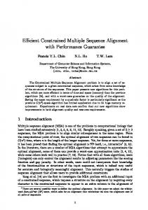
method. The same 5SD score cutoff was applied. This resulted in a set of 406 protein sequences with which to blind test the prediction methods. Alignments For each of the 480 training-set sequences, a multiple sequence alignment was constructed. For comparison, both BLAST and PSIBLAST were used to search the SWALL43 non-redundant protein sequence database, with a P-value cutoff of 0.0001. For PSIBLAST, three iterations were applied to search the sequence database. For each of the sequences found, the method described previously34 was applied to generate multiple sequence alignments. To compare the effect of different multiple sequence alignment methods, AMPS42 and CLUSTALW44 were both used. CLUSTALW44 was executed with default parameters while for AMPS,42 a BLOSUM62 matrix, and gap penalty of 10 were applied. The alignments were represented as profiles for input to the neural network and the profiles were scored in three ways:
Fig. 1. Outline of the final neural network method incorporated into the Jnet method.
prediction, with minimal concern that the test and training sets will be contaminated with proteins of similar sequence. In this work, the data were split randomly into seven sets to perform cross-validation tests. Blind Test Given the complexity of the network ensemble used for the final predictions (Fig. 1), it was essential that the prediction method was “blind tested” on a new set of proteins. The CASP3 proteins would have made for a good blind test. However, at the time this work was completed, the CASP3 experiment was six months old and the alignments would have contained new sequences. In addition, the CASP3 set only contained 17 structures and so has limited statistical value. The 480 proteins used to test and train the new prediction method were derived from the 1996 version of the PDB databank. Since then, more than 3,378 new protein structures have been released. This new set of structures provides the base for a separate non-redundant test set. Chains from the 3,378 proteins were compared pairwise by AMPS42 and the set screened such that no pair of sequences shared more than 5SD significance score. The new non-redundant sequences of known structure were then compared to the 480 proteins used to train the prediction
1. As frequency counts for each amino acid down a column in the alignment, expressed as a percentage of the total for a given column. This is the same approach as used by the PHD algorithm.17 2. Each residue in an alignment column was scored by its corresponding BLOSUM62 matrix score. The scores were then averaged based on the number of sequences in that column as in (1). This stopped each residue having an equal weight, instead using a weight based on that residue’s mutation score. 3. As a position specific profile, generated by the HMMER245 package. The multiple sequence alignment is represented as a profile HMM,46,47 with positionspecific scores to represent amino acids in the alignment. Figure 2 summarizes an attempt to improve the alignments obtained from PSI-BLAST by post-processing the result of the PSIBLAST search. As shown in Figure 2 full length sequences were taken from the PSIBLAST search, the alignment was then constructed by making successive global alignments to the profile by adding sequences in the order determined by the P-value scores from the initial PSIBLAST sequence search. At each iteration the ends of the alignment were trimmed, to force the global alignment method to represent the query sequence. In addition to the method summarized in Figure 2 each of the PSIBLAST alignments were also represented by the profiles in the PSIBLAST report file. Two profiles were extracted, the simple frequency counts (denoted in the PSIBLAST report as position characters, multiplied by 10 and rounded), and that denoted as the position-based scoring matrix (PSSM). Filtered Sequence Database PSIBLAST is an iterative searching method. During each iteration, it is possible for the searching profile to
504
J.A. CUFF AND G.J. BARTON
Fig. 2. search.
Outline of the progressive alignment method to align distantly related proteins from a profile based
become polluted with sequences that although show significant similarity to the query, ought not be included. This can be caused by low complexity sequence matching the query, or by matching sequences of biased composition. We applied SEG,48 to filter the search database, and so “masked out” regions of low complexity sequence. Coiled coil regions and transmembrane helices (TM’s) were also masked out from the database. Masking these regions was performed using HELIXFILT. HELIXFILT looks for heptad repeats for coils and also uses the membrane potentials from MEMSTAT49 to mask coils and transmembrane spans. HELIXFILT was kindly made available by Dr. D. Jones, and is also used as part of the PSIPRED39 method. The Neural Network In this work, the SNNS neural network package50 from Stuttgart University was applied. SNNS allows for rapid prototyping of neural networks, while also allowing incorporation of the resulting networks into an ANSI C function for use in stand-alone code. The network ensemble consisted of two artificial neural networks. The first was a network with a sliding window of 17 residues over each amino acid in the alignment, plus the addition of a conservation number6 as the input nodes. The network then comprised a further nine hidden nodes and three output nodes. The output from this network was windowed into 19 residues, plus a conservation number,6 which formed the input to the second network. This second network also had nine hidden nodes and three output nodes. Two hundred and fifty (250) epochs of Scaled Conjugate Gradient (SCC) training51 were applied, from an initial random weighting of node values of between 0.005 and ⫺0.005. No optimization was carried out for the number of training cycles.
For the PSIBLAST profiles and the HMMER profiles, only the windowed values for the profiles were applied, no conservation number was added. Consensus Combination of Prediction Methods The process of assessing the prediction methods resulted in different neural networks that were trained with different alignment data. Each of the networks were combined and the average taken for each predicted state, be it helix strand or coil. The outputs from each of the networks trained previously, were also taken and positions examined where the predicted state was identical in all methods. For positions where there was a “jury agreement” (identical predictions by all methods), the average Q3 accuracy was 82%. Residues where the predictions did not all agree were classified as “no jury” positions (see Fig. 3). Positions where there was a full agreement in the predicted state between the different neural network methods were taken as the final prediction. Positions where there was “no jury” were used to train a separate neural network. The final prediction was obtained by replacing the original “no jury” positions with the predictions from this network. Solvent Accessibility Prediction The alignments were also used to predict 2-state (exposed/buried) relative solvent accessible residues. Prediction accuracy was based on DSSP solvent accessibility definitions.52 Relative accessibility was calculated by dividing the DSSP accessibility by the accessibility for a Gly-XGly tripeptide given by the method of Rose and Dworkin.53 Three categories of relative accessibility were chosen for prediction: 25%, 5%, and 0% accessible. Neural networks were trained with profiles from the HMMER2 profiles and
MULTIPLE SEQUENCE ALIGNMENT PROFILES
505
Fig. 3. Positions where there is “no jury” (predictions do not all agree) are marked with a (*). These positions are re-predicted with a further neural network (the jury network (see Fig. 1). This network has only been trained with positions where there is “no jury.” Also shown is the relative solvent accessibility prediction at 25, 5, and 0% relative accessibility. “B” corresponds to buried residues, with “⫺” corresponding to exposed residues. Protein shown is Ribonuclease A (PDB57 code, 7rse58). DSSP52 relative solvent accessibility and secondary structure definitions are shown. Cross-validated prediction accuracy is 72.5% for this protein. (For reference PHD17 predicts this protein at 68.5% accuracy).
the PSSM (Position Specific Scoring Matrix) matrices from the PSIBLAST reports. The HMMER and PSIBLAST trained networks were also combined to give an average relative accessibility prediction. Confidence The highest scoring state from the outputs from the neural network was taken, and the score of the next highest predicted state subtracted: Confidence ⫽ integer共10 ⫻ 共outmax ⫺ outnext兲兲
(1)
17
This is similar to the method exploited by PHD.
Assessment of Secondary Structure Prediction Accuracy The accuracy of prediction was assessed by comparison to DSSP.52 The same 8- to 3-state reduction scheme was applied throughout the analysis to ensure that all relative changes in accuracy were consistent. This is important since application of different 8- to 3-state reduction methods can lead to apparent differences in accuracy of over 3% for the same predictions.34 E and B were taken as strand, H as helix and all other states were taken as coil. This removes the 310-helix state from the definition, but given that the 310-helix state represents a weak 1 kcal/mol hydrogen bond, this seems reasonable, as it does not
normally represent core secondary structure. Single residue -bridges (B) were included, as they do form part of core structures, however these structures are typically difficult to predict accurately. Removing single residue -bridges improves the apparent average Q3 prediction accuracy by at least 1% (data not shown). RESULTS AND DISCUSSION Two types of testing were performed. Seven (7) fold cross-validated predictions on 480 proteins are discussed first, then the results of “blind” tests on 406 new proteins not used in the development of the methods. Effect of Searching Method on Accuracy Table I shows the improvement obtained with a single two layer network and PSI-BLAST alignments from searching the filtered database, as opposed to that of BLAST against an un-filtered database. The improvement is of the order of 1%, for the 7-fold cross-validated experiment. This effect is not reflected in the “older” methods [DSC,13 PREDATOR,25 NNSSP,23 PHD17] (data not shown), as these methods were not trained with alignments extended by the sequences that are found using PSIBLAST. Effect of Alignment Method on Accuracy The effect of two different alignment methods, CLUSTALW and AMPS42 is summarised in Table II. AMPS may
506
J.A. CUFF AND G.J. BARTON
TABLE I. Comparison of BLAST Alignments Against Those Generated From a PSIBLAST of the SWALL43 Database, Compared to Those for a Database Filtered to Remove Coiled-coils, Low Complexity Segments and Transmembrane Helices (See Text)† Sequence searching method CLUSTALW alignments for BLAST against SWALL un-filtered database CLUSTALW alignments for PSIBLAST against a filtered database
Q3 accuracy 70.5% 71.6%
†
Figures are for Q3 accuracies based on a 7-fold cross-validated test on 480 proteins for the neural network prediction method.
TABLE II. Comparison of Profiles for Training Neural Networks† Method used to generate alignment profile Simple frequency profiles, alignments from CLUSTALW Simple frequency profiles, alignments from AMPS Blosum62 profiles, alignments from CLUSTALW Alignments with gaps (frequency profiles scored from CLUSTALW)
Q3 accuracy 71.6% 69.5% 70.6% 70.5%
Based on 480 proteins, cross-validated. AMPS42 was run with trees generated using the normalized alignment score from the pairwise sequence comparisons. All alignments have gaps in the primary sequence and any data directly below that gap in the alignment removed. For primary sequence and any data directly below that gap in the alignment removed. For the “Alignments with gaps” run, the alignments were left unmodified. This run was no more accurate, and took twice as long to train the networks for prediction.
TABLE III. All Values Are for 7-Fold Cross-validation on 480 Proteins Network
Q3 accuracy
Frequency profile alignments from CLUSTALW BLOSUM62 scored profile alignments from CLUSTALW PSIBLAST alignment profiles Arithmetic sum based on the above three networks
71.6% 70.8% 72.1% 73.4%
TABLE IV. Improving the Jnet Method Through the Use of Different Scoring Methods and Alignment Approaches† Matrix scoring and alignment method
Q3 accuracy (%)
BLOSUM62 profile CLUSTALW Frequency profile CLUSTALW Frequency profile PSIBLAST HMMER Profile CLUSTALW HMMER Profile Iterative Alignment (see Figure 2) PSSM PSIBLAST Numerical average of HMMER and PSSM PSIBLAST Jury/No Jury network (see Figs. 3 and 1)
70.8 71.6 72.1 74.4 74.3 75.2 76.5 76.9
†
These figures were generated from cross-validated predictions of the 480 non-redundant test set proteins.
†
be run in several different modes but in this study we used normalized alignment scores to generate the tree order, and the corresponding alignment. For the same sequences, predictions from alignments for CLUSTALW were 1.1% more accurate for the same cross-validated test than those for AMPS. This test shows CLUSTALW to be more favorable for generating multiple sequence alignments for secondary structure prediction. However, AMPS alignments are improved42 when randomization is performed to generate SD scores to define the sequence similarities, which can then be used to order the tree for the subsequent alignment. As this process is particularly computationally intensive it was not investigated here. Table II also summarizes the effect of two different methods for scoring the alignment profiles; simple frequency counting of residues in the alignment, and scoring positions by their BLOSUM62 matrix scores. The frequency matrix was 1% more accurate than the matrix scored by BLOSUM62 mutation scores regardless of the alignment method. Effect of Removing Gaps From Query Sequence All alignments discussed so far had gaps in the query sequence and residues in the corresponding column below each gap removed. Although this appears severe, it was standard practice for earlier prediction methods such as
NNSSP.23 As shown in Table II, including gaps in the query sequence during training and testing reduced the accuracy of prediction by 1.1%. This result was calculated based upon the ungapped sequence length, this way the ungapped and gapped alignments may be compared directly. This behavior may be explained, because regions where there are gaps in the query sequence, are most likely to be in the coil state, and as such have no effect on the prediction. The gapped alignments have another significant draw back in that the profiles are considerably larger than the profiles with the gaps removed, and as such take much longer to train. Effect of Training on PSIBLAST Profiles The same neural network architecture was trained with PSIBLAST profiles. PSIBLAST generates two types of profile, a simple frequency, and a position-based scoring matrix. Both were examined, and the results are shown in Table IV. The predictions based on the PSIBLAST alignments were 0.5% more accurate on average, than the predictions from the CLUSTALW alignment method (see Table III). When both predictions were combined in an arithmetic sum, the average accuracy rose to 73.4%, Table III. However, when the position specific scoring matrix of PSIBLAST was applied, the accuracy improved from 72.1% to 75.2%. The HMMER245 package was then used to re-score the CLUSTALW alignments. This raised the accuracy to 74.4% over 71.6%. The scoring schemes used in both PSIBLAST PSSM profile and the HMMER2 profiles are more sensitive than using simple frequency counts, as both apply
507
MULTIPLE SEQUENCE ALIGNMENT PROFILES
TABLE V. Comparison of Prediction Methods† Prediction method
Q3 accuracy (%)
Zpred6 DSC13 PREDATOR25 NNSSP23 PHD17 Jpred34 Jnet (this work)
62.0 70.6 70.7 72.3 73.3 74.6 76.4
†
Tested on the 406 new protein structures not used in the development of the Jnet method (see Methods).
scoring methods that use prior knowledge of amino acid relationships, derived from the BLOSUM62 matrix. In addition, the sequences are weighted by the amount of information they carry.40,45,47 This has the effect of removing redundancy in the alignments which has previously been shown to improve prediction accuracy.34 Position specific scoring schemes have also previously been shown to be more successful in sequence searching.42 The alignments from PSIBLAST gave more accurate predictions (75.2%) than those derived by the CLUSTALW alignments, re-scored as HMM profiles (74.4%). The alignment approach described in the Methods section (Fig. 2), was applied to retain the divergent sequences found by PSIBLAST. The predictions from these “progressive” alignments were compared to the original predictions derived from the CLUSTALW alignments. No significant improvement was found. The alignment method applied internally by PSIBLAST could not be improved upon in this work, as assessed by secondary structure prediction accuracy. Effect of Re-training “No Jury” Positions Table IV shows that keeping “jury positions” (positions where all neural network methods agree on a given predicted state) as the final prediction, and using a third neural network trained only on “no jury” positions (no agreement between all methods) improves the crossvalidated accuracy by 0.4% to 76.9%.
TABLE VI. Average Prediction Accuracies From 7-Fold Cross-Validation Experiments (Based on the 480 Protein Set) for 2-State Solvent Accessibility† Rel. Acc. (%)
PSIBLAST (%)
HMMER2 (%)
Combined [change] (%)
75.0 79.0 86.6
74.2 78.8 86.3
76.2 [⫹1.2] 79.8 [⫹0.8] 86.5 [⫺0.1]
25% 5% 0%
† “Rel. Acc.” corresponds to three thresholds of solvent accessibility, 25%, 5%, and 0% accessibility. For the combined method, a simple arithmetic sum between the PSIBLAST and HMMER2 network outputs was applied.
Fig. 4. Boxplots59 of per protein average secondary structure prediction accuracy (Q3) for each of the secondary structure prediction methods. Predictions are for the 406 blind test set. Boxplots show the variability of the median (white line), the dark box shows the limits of the middle half of the data. The upper and lower brackets mark the upper and lower quartiles. In this case the extreme data (outliers) have been removed for clarity.
TABLE VII. Improvement Assessment Between Jnet (This Work) and PHD,17 Broken Down into Helix, Strand, Coil, and SOV Accuracies. Predictions are for the 406 Proteins Not Used to Develop the Jnet Method Measurement of accuracy
Jnet (%)
PHD (%)
Improvement (%)
Relative solvent accessibility predictions for the different profiles are shown in Table VI. The results are for 7-fold cross validation experiments. Again the jury predictions based on an arithmetic sum between the PSIBLAST and HMMER profiles were more accurate (76.2%) than any single method. For reference, PHDacc achieved 75% average cross-validated accuracy for 2-states based on a 25% relative accessibility model.54
Q3 ␣-Helix accuracy -Strand accuracy Coil accuracy Sov256 SOV (␦ ⫽ 0%)54 SOV (␦ ⫽ 50%)54
76.4 78.4 63.9 80.6 74.2 61.6 82.9
73.3 76.8 63.8 76.5 69.8 57.8 79.6
⫹3.1 ⫹1.6 ⫹0.1 ⫹4.1 ⫹4.4 ⫹3.8 ⫹3.3
Blind Test of Prediction Methods
1.8% better than the Jpred34 consensus method. These figures were generated by application of the original PHD method, as described in Rost and Sander.17 As such the real accuracy of the modern day PHD method may well be higher. Table VII summarizes a closer investigation of the differences between PHD and the Jnet method. From these figures is is clear that while the Jnet method is more
Prediction of Solvent Accessibility
The results of a blind test of the new Jnet and other prediction methods that apply multiple sequence alignments for prediction are shown in Table V, and Figure 4. Predictions were made for 406 proteins not used to develop the methods (see Methods). On this set of 406 proteins, Jnet gave an average accuracy of 76.4%. This is 3.1% better than the best previous method (PHD, 73.3%) and
508
J.A. CUFF AND G.J. BARTON
Fig. 6. Jnet reliabilities compared to PHD reliabilities. The dashed line corresponds to PHD reliability. Average accuracies are compared to the corresponding residues with a confidence of greater or equal to the values shown on the x axis.
Fig. 5. Average secondary structure prediction accuracy (Q3), and percentage of residues against cumulative reliability score from the Jnet method. For example, for residues with reliability scores of greater or equal to 9, the average accuracy is 92.9%, and the percentage of residues with this score is 20.8%. Predictions are for the 406 blind test set proteins.
accurate than PHD, the -strand state is not predicted any more accurately by Jnet than PHD (0.1%). Most of the improvement comes from the clearer delineation of the helix and coil states, (1.6 and 4.1% respectively). A direct comparison to PSIPRED39 was not possible since PSIPRED was trained with over 1,300 protein structures, including test set proteins in the current study. For this reason, any PSIPRED predictions for the 406 proteins applied in this test would be biased. A true evaluation of PSIPRED and JNet will have to await protein structures not used to train either method. Reliability Scoring Figure 5 illustrates the results of reliability scoring scheme applied in the Jnet method. Those residues predicted with a confidence of 5 or greater had an average Q3 accuracy of 84%, and covered 68% of the total residues. Figures 6 and 7 show a comparison of the reliability scores for Jnet and the PHD prediction algorithm. The greatest benefits in accuracy for the new Jnet method arise for those positions assigned to reliability scores below 5. CONCLUSIONS In this paper, the effect of training a two-level neural network algorithm for protein secondary structure predic-
Fig. 7. Jnet residue coverage against reliability compared to PHD. The dashed line corresponds to PHD reliability. Average percentage of amino acids covered are compared to the corresponding residues with a confidence of greater or equal to the values shown on the x axis.
tion with the same sequences presented as different alignment profiles has been investigated. The general conclusions are: 1. By appropriate selection of database searching method, alignment algorithm and scoring scheme,
MULTIPLE SEQUENCE ALIGNMENT PROFILES
509
Fig. 8. Predictions from the improved Jpred2 server. Jpred2 prediction showing coiled coil predictions along side the improved Jnet predictions for the Manose binding lectin protein (PDB code 1afa). The multiple sequence alignment was generated from sequences found by PSIBLAST.
Transmembrane prediction by PHDhtm is also included. Also shown are relative solvent accessibility predictions by both PHD and Jnet, and coiled coil predictions by COILS60 and MultiCoil.61
the prediction accuracy for the same sequences using the same basic algorithm is improved by 7% points from 69.5% to 76.4%. Although the value of 76.4% accuracy is respectable, the final value of prediciton accuracy for this and other methods may only be obtained by future validation with further blind predictions. 2. Solvent accessibility prediction accuracy has been improved by 1.2% to 76.2% for a two state model, and also includes specific prediction of the 25, 5, and 0% relative accessibility states. 3. Confidence in prediction has been improved. Residues predicted with a confidence of 5 and greater, will be on average 84% accurate and cover 68% of residues. The average prediction accuracy per protein is 76.4% with a standard deviation of 8.4%.
4. In the years from 1993 to 1999, prediction accuracy has improved from 70.6%17 to over 76% (this work). Most of this improvement has come from more sophisticated use of sequence alignments, and improvements in database size rather than enhancements to the neural network algorithm. 5. The most dramatic improvements in prediction accuracy have come from the use of PSIBLAST and the application of position specific scoring profiles in preference to profiles derived from global multiple alignment methods such as CLUSTALW and AMPS. Given the expansion of structural genomics projects, which aim to solve protein structures much more rapidly, the exploitation of these data will only extend the ability to predict protein structure ever more accurately.
510
J.A. CUFF AND G.J. BARTON
AVAILABILITY ANSI C source code for the neural network prediction method (Jnet) designed as part of this work is available from http://barton.ebi.ac.uk/ and as down-loadable binaries for all the major UNIX platforms. The Jnet method has been incorporated into an improved version of the Jpred55 consensus secondary structure prediction server as shown in Figure 8. The improved consensus prediction server is also accessible from http://barton.ebi.ac.uk/. ACKNOWLEDGMENTS The authors thank Dr. David Jones for many insightful discussions, and for making the HELIXFILT program for filtering sequence databases available. We would also thank Prof. Sean Eddy for making the HMMer2 package so widely available and Dr. Steve Searle for aiding the development of the C program Jnet. Finally, we thank all of the authors of the different secondary structure prediction methods that were applied. J.C. is an Oxford Centre for Molecular Sciences/MRC Student. REFERENCES 1. Jones DT, Taylor WR, Thornton JM. A new approach to protein fold recognition. Nature 1992;358:86 – 89. 2. Rost B. Protein fold recognition by prediction-based threading. J Mol Biol 1997;270:1–10. 3. Russell RB, Copley RR, Barton GJ. Protein fold recognition by mapping predicted secondary structures. J Mol Biol 1996;259:349 – 365. 4. Russell RB, Saqi MAS, Sayle RA, Bates PA, Sternberg MJE. Recognition of analogous and homologous protein folds: Analysis of sequence and structure conservation. J Mol Biol 1997;269:423– 439. 5. Fischer D, Eisenberg D. Protein fold recognition using sequencederived potentials. Protein Sci 1996;5:947–955. 6. Zvelebil MJJM, Barton GJ, Taylor WR, Sternberg MJE. Prediction of protein secondary and active sites using the alignment of homologous sequences. J Mol Biol 1987;195:957–961. 7. Garnier J, Osguthorpe DJ, Robson B. Analysis and implications of simple methods for predicting the secondary structure of globular proteins. J Mol Biol 1978;120:97–120. 8. Chou PY, Fasman GD. Conformational parameters for amino acids in helical, -sheet, and random coil regions calculated from proteins. Biochemistry 1974;13:211–222. 9. Garnier J, Gibrat J, Robson B. GOR method for predicting protein secondary structure from amino acid sequence. Methods Enzymol 1996;266:540 –553. 10. Gibrat JF, Garnier J, Robson B. Further developments of protein secondary structure prediction using information theory. New parameters and consideration of residue pairs. J Mol Biol 1987;198: 425– 443. 11. Nishikawa K, Nogughi T. Predicting protein secondary structure based on amino acid sequence. Method Enzymol 1995;202:31– 44. 12. Lim VI. Algorithms for prediction of ␣ helices and  structural regions in globular proteins. J Mol Biol 1974;88:873– 894. 13. King RD, Sternberg MJE. Identification and application of the concepts important for accurate and reliable protein secondary structure prediction. Protein Sci 1996;5:2298 –2310. 14. King R, Sternberg MJE. Machine learning approach for the prediction of protein secondary structure. J Mol Biol 1990;216:441– 457. 15. Muggleton S, King R, Sternberg MJE. Protein secondary structure prediction using logic-based machine learning. Protein Eng 1992;5:647– 657. 16. Qian N, Sejnowski TJ. Predicting the secondary structure of globular proteins using neural network models. J Mol Biol 1988; 202:865– 884. 17. Rost B, Sander C. Prediction of protein secondary structure at better than 70% accuracy. J Mol Biol 1993;232:584 –599.
18. Holley HL, Karplus M. Protein secondary structure prediction with a neural network. Proc Natl Acad Sci 1989;86:152–156. 19. Kneller DG, Cohen FE, Langridge R. Improvements in protein secondary structure prediction by an enhanced neural network. J Mol Biol 1990;1:171–182. 20. Riis SK, Krogh A. Improving prediction of protein secondary structure using structured neural networks and multiple sequence alignments. J Comput Biol 1996;1:163–183. 21. Chandonia JM, Karplus M. The importance of larger data sets for protein secondary structure prediction with neural networks. Protein Sci 1996;5:768 –774. 22. Chandonia JM, Karplus M. New methods for accurate prediction of protein secondary structure. Proteins 1999;35:293–306. 23. Salamov AA, Solovyev VV. Prediction of protein secondary structure by combining nearest-neighbor algorithms and multiple sequence alignments. J Mol Biol 1995;247:11–15. 24. Rychlewski L, Godzik A. Secondary structure prediction using segment similarity. Protein Eng 1997;10:1143–1153. 25. Frishman D, Argos P. Incorporation of non-local interactions in protein secondary structure prediction from the amino acid sequence. Protein Eng 1996;9:133–142. 26. Yi T, Lander ES. Protein secondary structure prediction using nearest neighbor methods. J Mol Biol 1993;232:1117–1129. 27. Levin JM. Exploring the limits of nearest neighbour secondary structure prediction. Protein Eng 1997;10:771–776. 28. Geourjon C, Deleage G. Sopma: Significant improvements in protein secondary structure prediction by consensus prediction from multiple alignments. Comp Appl Biosci 1995;11:681– 684. 29. Goldman N, Thorne J, Jones DT. Using evolutionary trees in protein secondary structure prediction and other comparative sequence analyses. J Mol Biol 1996;263:196 –208. 30. Lio P, Goldman N, Jones DT. PASSML: combining evolutionary inference and protein secondary structure prediction. Bioinformatics 1998;8:726 –733. 31. Mehta PK, Heringa J, Argos P. A simple and fast approach to prediction of protein secondary structure from multiply aligned sequences with accuracy above 70%. Protein Sci 1995;4:2517– 2525. 32. Zimmermann K, Gibrat JF. In unison: regularization of protein secondary structure predictions that makes use of multiple sequence alignments. Protein Eng 1998;10:861– 865. 33. Viswanadhan VN, Denckla B, Weinstein JN. New joint prediction algorithm (Q7-JASEP) improves the prediction of protein secondary structure. Biochemistry 1991;46:11164 –11172. 34. Cuff JA, Barton GJ. Evaluation and improvement of multiple sequence methods for protein secondary structure prediction. Proteins 1999;34:508 –519. 35. Biou V, Gilbrat JF, Robson B, Garnier J. Secondary structure prediction: combination of three different methods. Protein Eng 1995;2:185–191. 36. Guermeur Y, Geourjon C, Gallinari P, Deleage G. Improved performance in protein secondary structure prediction by inhomogeneous score combination. Bioinformatics 1999;5:413– 421. 37. Moult J, Hubbard T, Bryant SH, Fidelis K, Pedersen JT. Critical assessment of methods of protein structure prediction (CASP): Round II. Proteins Suppl 1997;1:1–230. 38. Moult J, Hubbard T, Pedersen JT, Fidelis K. Third Meeting on the critical assessment of techniques for protein structure prediction: Asilomar Conference Centre, December 13–17. http://predictioncenter.llnl.gov/casp3/Casp3.html, 1998. 39. Jones DT. Prediction of protein secondary structure at 77% accuracy based on PSI-BLAST derived sequence profiles. Third meeting on the critical assessment of techniques for protein structure prediction: Asilomar Conference Centre, December 13–17, 1998. 40. Altshul SF, Madden TL, Schaffer AA, Zhang JH, Zhang Z, Miller W, Lipman DJ. Gapped BLAST and PSI-BLAST: a new generation of protein database search programs. Nucleic Acid Res 1997;25: 3389 –3402. 41. Park J, Karplus K, Barrett C, Hughey R, Haussler D, Hubbard T, Chothia C. Sequence comparisons using multiple sequences detect three times as many remote homologues as pairwise methods. J Mol Biol 1998;284:1201–1210. 42. Barton GJ. Protein multiple sequence alignment and flexible pattern matching. Methods Enzymol 1990;183:403– 428. 43. Bairoch A, Apweiler R. The SWISS–PROT protein sequence data bank and its supplement TrEMBL in 1999. Nucleic Acids Res 1998;27:49 –54.
MULTIPLE SEQUENCE ALIGNMENT PROFILES 44. Thompson JD, Higgins DG, Gibson TJ. CLUSTAL W: improving the sensitivity of progressive multiple sequence alignment through sequence weighting, positions-specific gap penalties and weight matrix choice. Nucleic Acids Res 1994;22:4673– 4680. 45. Eddy SR. HMMer2. http://hummer.wustl.edu/, 1999. 46. Krogh A, Brown M, Mian IS, Sjolander K, Haussler D. Hidden markov models in computational biology. J Mol Biol 1994;235: 1501–1531. 47. Durbin R, Eddy S, Krogh A, Mitchison G. Biological sequence analysis. Cambridge: Cambridge University Press, 1998. 48. Wootton JC, Federhen S. Statistics of local complexity in amino acid sequences and sequence databases. Comput Chem 1993;17: 149 –163. 49. Jones DT, Taylor WR, Thornton JM. A model recognition approach to the prediction of all-helical membrane protein structure and topology. Biochemistry 1994;33:3038 –3049. 50. Zell A, Mamier G, Vogt M, et al. The SNNS users manual version 4.1. http://www.informatik.uni-stuttgart.de/ipvr/bv/projekte/snns/ UserManual/UserManual.html, 1995. 51. Moller MF. A scaled conjugate gradient algorithm for fast supervised learning. Neural Networks, 1993;6:525–533. 52. Kabsch W, Sander C. A dictionary of protein secondary structure. Biopolymers 1983;22:2577–2637. 53. Rose GD, Dworkin JE. The hydrophobicity profile. In: Fasman
54. 55. 56. 57. 58. 59. 60. 61.
511
GD, editor. Prediction of protein structure and the principles of protein conformation, 625– 634. New York: Plenum Press, NY, 10013, 1989. Rost B, Sander C, Schneider R. Redefining the goals of protein secondary structure prediction. J Mol Biol 1994;235:13–26. Cuff JA, Clamp ME, Siddiqui AS, Finlay M, Barton GJ. Jpred: a consensus secondary structure prediction server. Bioinformatics 1998;14:892– 893. Zemla A, Vencolvas C, Fidelis K, Rost B. A modified definition of SOV, a segment-based measure for protein secondary structure prediction assessment. Proteins 1999;34:220 –223. Bernstein FC, Koetzle TF, Williams GJB, et al. The protein data bank: a computer based archival file for macromolecular structures. J Mol Biol 1977;112:535–542. Wlodawer A, Bott R, Sjolin L. The refined crystal structure of ribonuclease A at 2.0 A resolution. J Biol Chem 1982;257:1325– 1332. McGill R, Tukey JW, Larsen WA. Variations of box plots. The American Statistician 1978;32:12–16. Lupas A, Van Dyke M, Stock J. Predicting coiled coils from protein sequences. Science 1991;252:1162–1164. Wolf E, Kim PS, Berger B. MultiCoil: a program for predicting two- and three-stranded coiled coils. Protein Sci 1997;6:1178 – 1189.