be found in KDAC (Keithley Data Acquisition and Control) manual supplied by the manufacturer. .... Gibbs free energy using any standard thermodynamic model (e.g., Margules, Van. 45 ... The Gibbs-Duhem equation for binary mixtures.
APPLICATION OF NEURAL NETWORK CONTROL TO DISTILLATION by
PRIYABRATA DUTTA, B.Tech., M.Tech. A DISSERTATION IN CHEMICAL ENGINEERING Submitted to the Graduate Faculty of Texas Tech University in Partial Fulfillment of the Requirements for the Degree of DOCTOR OF PHILOSOPHY Approved
ACKNOWLEDGMENTS
I wish to take this opportunity to convey my sincere thanks to my research advisor, Dr. Russell Rhinehart. His encouragement, suggestions and guidance in many matters have greatly helped me in achieving my academic goals. What I like most is his unique way of teaching, way of providing hints and making us understand the problem and the direction of solution in a lucid and transparent manner. I acknowledge him for being with me throughout my research. His friendly yet professional attitude towards students has made him a 'superb professor' in my eyes. I feel privileged to get an opportunity to work with an advisor like 'Russ\ I am thankful to Dr. James B. Riggs for giving me admission to Texas Tech and providing me an opportunity to work in my desired field. I would also like to give my special thanks to Dr. Brian Oldham for opening a door to the Computer Science Department. His calm disposition and brief and to the point answer to all my questions have always been an extra encouragement to me. This dissertation would not have been complete without the corrections by Dr. Robert Bethea. I appreciate his time, effort and interest in the preparation of this dissertation. I also wish to convey my thanks to Dr. Hua Li for his advice, questions and comments as my committee member. Thanks are also extended to the members of the Process Control and Optimization Consortium at Texas Tech University for financial support of this work.
Although, I did not get much
opportunity to take many chemical engineering courses
with the professors in this
department, I never felt out of place at any time. For this, my sincere thanks go to Dr. Narayan, Dr. Tock, Dr. Mann, Dr. Heichelheim and Dr. Wiesner. ii
I acknowledge Mr. Robert Spruill for extending his helping hand during the phase of 'instrumental trouble' of the experimental setup. Tammy and Mary, the two pillars of administration, will always be remembered by me as the best two persons in the Chemical Engineering Department. Thanks are also due to Sandeep Lai, Siva, Ramesh, Mahesh, Ganesh, Abe, Bala, Scott and Joe for their friendship during my stay at Tech. My last one and a half year stay at Lubbock would not be any better without the assistance of my lovely wife 'Adity'. Besides her moral support and encouragement, her delicious cooking kept me 'going and going' during the last phase of the long experimental runs. Finally, I would like to say that it would not be possible for me to pursue my graduate studies in the US without the support of my mom, my brothers and sisters across the ocean.
in
TABLE OF CONTENTS
ACKNOWLEDGEMENTS ABSTRACT LIST OF TABLES LIST OF FIGURES NOMENCLATURE
ii vi viii ix xii
CHAPTER I INTRODUCTION
1
II
LITERATURE SURVEY 2.1 Distillation Control 2.1.1 Importance 2.1.2 Objectives 2.1.3 Constraints 2.1.4 Distillation Control Literature 2.2 Literature on Linear and Nonlinear Control 2.2.1 Linear Model Based Control 2.2.2 Nonlinear Model Based Control 2.3 Neural Network Control 2.3.1 Importance of Neural Networks in Control 2.3.2 Literature on Neural Network Control 2.3.3 An Introduction to Neural Networks 2.3.4 Training of Neural Networks 2.3.4.1 Backpropagation 2.3.4.2 Optimization Approach 2.4 Self-Tuning Filter
IH
EXPERIMENTAL SETUP AND SIMULATOR 3.1 Experimental Setup 3.1.1 Distillation Unit 3.1.2 Instrumentation 3.1.3 Data Acquisition and Control System 3.1.4 Interfacing Program Development 3.1.5 Control Difficulties 3.2 Simulator 3.2.1 Model Equations 3.2.2 Assumptions 3.2.3 Design and Operating Conditions
IV
CONTROLLER DEVELOPMENT 4.1 Neural Network Model Inverse and State Prediction IV
7 7 7 7 8 8 13 13 15 17 17 18 19 19 23 25 28 32
32 32 35 38 38 40 42 42 44 45 48
43
4 2 Neural Network Model and Gain Prediction 4.3 Optimization and Constraint Handling (HRO) V
CONTROL RESULTS 5.1 Simulator Results 5.1.1 Distillation Control with NN Gain Prediction 5.1.2 Distillation Control with Gain Prediction (Constrained Control Mode) 5.2 Experimental Results 5.2.1 NN Control in State Inverse Mode on SISO systems (Heaters) 5.2.2 NN Control in State Inverse Mode on Distillation Column 5.2.2.1 Setpoint Tracking 5.2.2.2 Disturbance Rejection 5.2.3 NN Control of Distillation Column in Gain Prediction Mode 5.2.3.1 Setpoint Tracking 5.2.3.2 Disturbance Rejection 5.2.4 Constrained Control of Distillation Column with NN Gain Prediction 5.2.5 Process Model Mismatch 5.2.6 ATV Results
VI
VII
COMPARISON OF CONTROL RESULTS 6.1 Performance Comparison 6.2 Other Issues CONCLUSION AND RECOMMENDATION 7.1 Conclusions 7.2 Recommendations
REFERENCES APPENDICES A. PMBC.ACC and [DMC]™ CONTROL RESULTS B. INSTRUMENT CALIBRATION AND PROPERTY CORRELATION C. SOFTWARE
A
setpoint
D)
i —
CD "D
controlled output
c D O
130-1
.CD 3500 -Q CO
120-
co
CD CO
4000
>
CD QL
-3000
CD *-
"D CD • * - •
manipulated variable
£_ 90-
J"
JO D -2500 .9-
c
I
V
CO
E -2000
80
50
100
150
200
250
300
time (minutes)
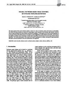
Figure 5.10. Neural network control on feed preheater.
84
350
-+1500 400
errors or parameter errors, the controller is able to return the process to the setpoint with zero offset in a smooth manner. The manipulated variable moves are much larger at the temperature level of 130 and 140°F in comparison to 120°F. This variation of movements in manipulated variables further illustrates the "gain scheduling" inherent in this controller. A quantitative analysis of the controller performance is shown in Table 5.3. The values of Integral of Square Error (ISE), Integral of the Absolute Error (IAE), Integral of the Timeweighted Absolute Error (ITAE) and total manipulated variable movements are calculated over a time interval of 25 minutes, after the setpoint changes are introduced. This is approximately the maximum time taken by the controller to bring the process to its new setpoint.
Table 5.3 Comparative Study on Feed Preheater Control
Setpoint Change 130-140°F
Setpoint Change 130-120°F
PI
TMC
MPC
NN
PI
TMC
MPC
NN
Rise time (min.)
18.0
23.5
7.5
6.0
9.0
5.0
7.5
4.0
Overshoot
0.84
0.9
1.02
1.28
-2.81
-6.27
-1.02
-0.8
ISE (°F) 2 .min
940
840
630
480
910
870
630
290
IAE (°F) .min
170
140
100
85
155
165
100
60
ITAE
1225
845
535
485
1130
1845
535
385
175
395
710
2385
175
1695
710
195
(°F)
(°F).min
ZI A w
2
(counts)
85
Although the artificial neural network (the steady state form as used) does not take into account time delays that affect the dynamics of the system (i.e., the NN 'believes' that input changes produce an immediate output change), the use of a lower value of the integral gain (K2) helped in restraining a large overshoot, but still eliminated the offset successfully. As a result, the controlled output is found to be more aggressive, reducing the rise-time, as compared to the linear controller. The neural-network model-based controller is able to produce low ISE (Integral of the Square error), IAE (Integral of the Absolute Error) and ITAE (Integral of the Time-weighted Absolute Error). The neural network controller's success can solely be attributed to its capability to adapt its gain according to the process gain changes. Since the process gains differ significantly (almost 12-14 times) at the 140°F level in comparison to 120°F, the manipulated variable movement also adjusts itself accordingly. As a result, Table 5.3 shows a higher cumulative of absolute manipulated variable movement ( ^ l A w b
m
^N control performance (almost
12 times that of PI). While not shown here, operating experience qualitatively indicates that regulatory performance gives a similar result. A similar NN model-based inverse of a state-prediction controller is implemented on the reflux heater as well. Figure 5.11 shows the neural network training result. The performance of this controller in response to setpoint changes and disturbances is shown in Figure 5.12. In this experiment, reflux flowrate changes are given from 40 to 35 ml/min, 35 to 45 ml/min and 45 to 40 ml/min at time t = 275, 295 and 335 minutes, respectively, along with the various setpoint changes. The neural network controllers, representing the inverse of a steady-state of the process and generic model control law as the reference system trajectory, show excellent 86
2100-
^
2000-
co c D O
1900-1
A
c o ^3
1800-
o -o
>**
y*
CD Q. 0)
1700-
O
1600-
M
1500-
140O 1400
— I
1500
1
1600
— I
1700
1800
1900
2000
training data (counts)
Figure 5.11. Training result on manipulated variable of reflux preheater.
87
2100
180
5000
170-
controlled output
4500
CD "O
150-
CD L_ D •*-> CO CD
140-
a E CD
•*-> X D
'ciT
'•Aw^/*^*^^^*
160 LL
4000 g
setpoint
{^
.CD
3500 -2
cc cc
7
130-
"k_
>
3000 "O 120-
r«m-,
k_
0.35
Q. "CD •D
O
034
E 0.33-
0.32 0.32
0.33
0.34
0.35
0.36
0.37
0.38
training data (boilup rate,lbmoles/hr)
Figure 5.13. Training result on manipulated variables in inverse of steady-state prediction mode, (a) Vapor boilup rate.
90
0.39
0.23
^ A CO CD
0.22-
0.21-
O
F
.Q ^—' C
0.2-
o
0.19-
^ _ l
o
"D CD
O £
0.18-
0.160.15-
0.14 014
0.15
016
0.17
018
0.19
0.2
training data (reflux rate,lbmoles/hr)
Figure 5.13. Continued, (b) Reflux rate.
91
021
0.22
0.23
For all the runs, the operating conditions are tabulated and the controller performance is presented with the figures of the controlled variables, i.e., the top and bottom compositions and the manipulated variables, i.e., the reflux flow rate and the vapor boilup after converting 'counts' to 'gmoles/hr' using the correlation as described in Appendix C and Appendix D. Table 5.4 lists the experimental runs discussed in this section. These sets of experiments are done to reproduce Pandit's PMBC (1991) and Gupta's DMC and Advanced Classical Control (ACC) (Gupta, 1994) experimental runs for a one-on-one comparison of control techniques. Both setpoint tracking and disturbance rejection results are discussed below.
5.2.2.1 Setpoint Tracking Figures 5.14(a), 5.14(b) and 5.14(c) show the column performance for simultaneous setpoint changes in the top and bottom compositions. The conditions are summarized in Table 5.5. As seen in Figure 5.14(a) and 5.14(b), the top composition setpoint is changed from 86.0 mole% to 91.0 mole% methanol, while the bottom composition setpoint is changed from 1.4 mole% to 5.0 mole% methanol. Figure 5.14(c) shows the changes in manipulated variables during the run. The column is started in an open-loop fashion by providing a constant boilup rate of 162 gmoles/hr. Once the vapor starts condensing at the condenser, the reflux pump is started at a constant rate of 78 gmoles/hr. At about 60 minutes, the controllers are put into automatic mode with setpoints of 86 mole% for the top composition and 1.4 mole% for the bottom
92
Table 5.4. Synopsis of Experimental Runs in Control Performance Study
Objective
Case Number
Setpoint Tracking
1
Top : 86% to 91% Methanol Bottom : 1.4% to 5% Methanol
Disturbance Rejection
2
Feed Composition Disturbance (20% to 35% Methanol (+55% relative)
3
Feed Composition Disturbance (30% to 20% Methanol (-40% relative)
»5
Changes Made
93
Table 5.5. Setpoint tracking with neural network control in inverse of the state prediction mode (Case 1)
Operating Characteristics Feed Rate (mols/hr.)
Initial Operating Conditions
Final Operating Conditions
220.0
220.0
Feed Composition (mol % methanol)
20.0
20.0
Feed Temperature (deg F)
100.0
100.0
73.0
101.0
Reflux Rate (mols/hr.) Reflux Temperature (deg F)
110.0
110.0
Vapor Boilup (mols/hr.)
156.0
168.0
Top Composition (mol % methanol)
86.0
91.0
Bottom Composition (mol % methanol)
1.4
5.0
94
1.05
1-1 steady-state target
**= 0.95"o E,
c q
^/Yv^^'^^V^
0.9-
*+^
'co O 0.85Q.
E o o
0.8-
Q.
O 0.750.7
50
100
150 200 time (minutes)
250
Figure 5.14. Setpoint tracking with neural network control in inverse o f steady-state prediction mode (Case 1). (a) Top composition.
95
300
0.15
o a 0.12 o E
^ o
steady-state target
0.09
50
100
150 200 time (minutes)
Figure 5.14. Continued, (b) Bottom composition.
96
250
300
200 £
180
|
160
3 «T 140 (D
o. 120H A 100H
1 80 2
60H 40 0
50
100
150 200 time (minutes)
250
Figure 5.14. Continued, (c) Manipulated variables.
97
300
composition. At 150 minutes, simultaneous setpoint changes to 91 mole% and 5 mole% are given for the top and bottom compositions, respectively. After the changes are made, the top composition takes about 50 minutes to settle down to the new setpoint while the bottom composition takes about 100 minutes. The manipulated variable action is shown in Figure 5.14(c). Immediately after the controllers are put into automatic, the manipulated variables start moving to maintain the process at the setpoints. Sharp step changes in the manipulated variables are also expected at the point of simultaneous setpoint changes. Figures 5.14(a) and 5.14(b) also show the steady-state target values (i.e., the outputs of the GMC law) for the top and bottom compositions. The values of KXD, K2D, K]B, K2B (Equation 4.6 and 4.7) as used in this experimental run are 1.1, 0.028 min -1 , 1.1, 0.02 min"1, respectively. These parameter values are achieved by "field tuning" online, for good servo control, as an experienced operator would tune conventional decoupled PI controllers. This tuning took a total of 10 runs. It is observed that the integral values (i.e., K2D and K2B) produce maximum effect in terms of the aggressiveness of the controller and eliminating the offset. The process responds slowly to the changes of the manipulated variables, suggesting that the process is primarily an integrating process. An increase in the proportional values (i.e., KXD and KXB) requires a decrease in the integral values in order to keep the process away from the constraint and to avoid any integral windup. Lower values of the integral terms would result in an offset. It is also observed that because of the relatively faster dynamics of the top composition, the performance of the dual-composition control mode (in terms of rise time, settling time, etc.) depends mainly on the tuning of the bottom 98
composition control loop. The tuning ranges of KXD,KXBJK2D and K2B explored on the experiment are (0.7 -2.0), (0.7 - 2.0), (0.015-0.05)min"1 and (0.015 - 0.05)min~\ respectively. The initial deviations in the steady-state target valuesfromthe actual compositions at the transfer to the automatic mode, as observed in Figures 5.14(a) and 5.14(b), are due to the process-model mismatch represented by the bias terms of Equation 4.6 and 4.7. The controller has been able to accommodate this process-model mismatch and maintain both the top and bottom compositions successfully at their respective setpoints.
5.2.2.2 Disturbance Rejection Two types of disturbances were investigated by the previous researchers on this particular column. One is the feed-flowrate disturbance and another is the feedcomposition disturbance. It has been observed that a feed flowrate disturbance (+20% or -20%) from 220 gmoles/hr (base value of the present experiment) does not produce significant deviations in the top and bottom compositions compared to the feedcomposition disturbance. Therefore, in this research, only feed composition disturbances are introduced and analyzed for the control study. The feed composition disturbances are introduced according to Case 2 and Case 3 shown in Table 5.4. The detailed operating conditions during these experimental runs are shown in Tables 5.6 and 5.7. Figures 5.15(a) and 5.15(b) show the control results for a feed-composition disturbance from 20 mole% to 35 mole% (+55% relative) methanol, introduced at a time about 70 minutes intto the run. Because of this disturbance, the top
99
Table 5.6. Disturbance rejection with neural network control in inverse of the state prediction mode (Case 2)
Operating Characteristics Feed Rate (mols/hr.)
Initial Operating Conditions
Final Operating Conditions
220.0
220.0
Feed Composition (mol % methanol)
20.0
35.0
Feed Temperature (deg F)
100.0
100.0
73.0
58.0
110.0
110.0
156.0
160.0
90.0
90.0
2.1
2.1
Reflux Rate (mols/hr.) Reflux Temperature (deg F) Vapor Boilup (mols/hr.) Top Composition (mol % methanol) Bottom Composition (mol % methanol)
100
1.05
1O
top composition
CO k—
0.95-
®.
o
g
^A^^WVA^^
c o
0.9-
O Q.
0.85
^ W r f ^
E o O
a o
0.8
feed composition disturbance / (20-35%) at t=70
0.75
0.7-
-1—
50
100
150
200
time (minutes)
Figure 5.15. Disturbance rejection with neural network control in inverse of steady-state prediction mode (Case 2). (a) Top composition.
101
250
a 05
100
150
time(minutes)
Figure 5.15. Continued, (b) Bottom composition.
102
250
200-
180-
O
160-1-
E
I
^\ Vff*
0.85-
Q.
E 8
0.8H
feed composition (30-20%) disturbance att=75
Q. O 0.75-
0.7-
50
100
150
200
250
time (minutes)
Figure 5.20. Disturbance rejection with neural network control in gain prediction mode (case 3). (a) Top composition.
126
300
0.05
O
2
0.04-
o E, c
bottom composition 0.03-
O CO
o
Q.
E o o E o o
0.02-
feed composition (30-20%) disturbance at t=75
0.01-
A
50
100
150
200
time (minutes)
Figure 5.20. Continued, (b) Bottom Composition.
127
250
300
200-
.c
180-
~CD
0
E
160-
U)
^—"' CO 0 •*-• C O l_
140-
Q. _3
120-
boilup
reflux
o A •o
100-
c x 2
feed composition (30-20%) disturbance at t=75
60H 40 50
100
150
200
time (minutes) Figure 5.20. Continued, (c) Manipulated variables.
128
250
300
seen that the change in manipulated variable movements, particularly the reflux changes, are significantly more in the gain prediction mode, even though the composition deviations are less. This can also be due to the difference in tuning. However, no significant difference is observed in the change of manipulated variable movements in response to the setpoint changes.
5.2.4 Constrained Control of Distillation Column with NN Gain Prediction In section 4.2, it is stated that the control strategy developed in this research based on the novel gain-prediction approach along with the Heuristic Random Optimizer has the ability to handle constraints. Simulation results verify this claim. However, experimental demonstration is also needed to verify its performance in a real-time situation. As any other real process, the present experimental system also possesses few operational constraints. The heater to the boiler has a maximum power limit. The reflux rate has a maximum limit corresponding to maximum vapor boilup. A minimum reflux rate has to be maintained for satisfactory operation of the distillation column. Therefore, the constraints are mainly on the manipulated variables. The constrained control performance is tested by putting an upper limit of the vapor boilup close to the maximum power. In this experiment, an upper constraint for the boilup rate is set at 0.37 lbmoles/hr (i.e., V < 0.37 lbmoles/hr). The reflux is kept intentionally out of any feasible constraints. Figures 5.21(a) and (b) show the result of the constraint control. A feedcomposition disturbance (20 mole% to 50 mole% methanol) is introduced at 125 minutes.
129
1.05
top composition
O
CO
-2> o E, c o CO O Q.
setpoint
0.95
'^ivV^
0.9-
0.B5
E o O Q. O +->
0.8
feed composition (50-20%) disturbance at t = 3 3 5
feed composition (20-50%) disturbance at t = 1 2 5
0.750.7+ 0
r 50
100
150
200
250
300
350
400
450
time (minutes)
Figure 5.21. Constrained control with NN gain prediction using feed composition disturbance, (a) Top composition.
130
500
0.06
o
0.05-
CO
_CD
O
E, c q
0.04
CO O Q.
0.03
E
o o E o *s o A
O02-
0.01-
'i0
feed composition (20-50%) disturbance at t=125 f e e d composition (50-20%) disturbance at t=335 —I
50
1
1
1
1
1
100
150
200
250
300
I
—
350
400
time (minutes)
Figure 5.21. Continued, (b) Bottom composition.
131
450
500
180 160-
•5
o E 3
boilup
140120-
CO
reflux
CD
"co Q. J| O A ~0 C
IOO80-|
60-
CO
X _D »*—
40-
Q)
feed composition (50-20%)
feed composition (20-50%) disturbance at t= 125
disturbance at t=335
20-
50
100
150
200
250
300
350
400
time (minutes) Figure 5.21. Continued, (c) Manipulated variables.
132
450
500
Both the top and bottom compositions are deviated higher than the setpoints. To keep the compositions at their setpoints, the boilup rate starts increasing and the refux rate starts decreasing. However, Figure 5.21(c) shows that the boilup hits the constraint at about 160 minutes and the reflux rate settles down to a value so as to keep the objective function (Equation 4.15)
to a minimum. Similar to the simulation result (as shown in Figure
5.4(a)), it is observed that a negative deviation of the top composition from its setpoint and a positive deviation of the bottom composition from its setpoint are maintained when the boilup rate maintains the constraint. The controller is able to come out of the constraint when the feed-composition is changed back to 20% and eliminates the offsets in the top and bottom compositions. The controller also shows no delay or windup while coming out of the constraint. Interestingly, this experimental run also shows the presence of nonlinearity in the process. It is known that a distillation column shows lower gain at high purity and the higher gain at low purity. Here, a positive feed-composition disturbance shows lower change at the top purity above 90 mole% (i.e., higher purity for the top), but higher change for the bottom purity above 2.7 mole % (i.e., lower purity for the bottom). An exactly opposite response is observed when the negative feed-composition disturbance is given at time t=335 minutes. Table 5.11 shows a comprehensive evaluation of overall material balance and component material balance closures during the various experimental runs conducted in this study. The errors are calculated based on the duration of steady-state operation. The
133
Table 5.11. Material Balance Closure in Experiments 5.14
5.15
5.16
5.18
5.19
5.20
5.21
60
60
30
120
60
60
30
220
220
220
220
220
220
220
Feed Composition (methanol mole % )
20
35
20
20
35
20
20
Average Distillate Flowrate (gmoles/hr)
30
55
42
34
58
38
42
170
160
175
180
150
160
145
Top Composition (methanol mole % )
91
90
90
91
90
90
90
Bottom Composition (methanol mole %)
5
2
2.5
5
2
2.5
3
Overall Material Balance Error (%)
9.1
2.3
1.4
2.7
5.5
10.0
15.0
Component Material Balance Error (%) (Methanol)
18.6
31.5
4.2
9.2
28.3
13.2
4.2
Experimental Figure Number Period of Estimation (minutes) Feed Flowrate (gmoles/hr)
Average Bottom Product Flowrate (gmoles/hr)
134
average distillate flowrate, bottom product flowrate, top and bottom product compositions are also shown in this table.
5.2.5 Process Model Mismatch Expectedly, perhaps performance of the model-based controller should largely depend on the validity of the process model. In this study, the neural network model is generated based on steady-state data sets derived from a simulator. The simulator has i
various idealizations and assumptions (as discussed in section 3.2.2) which differ from the real environment. The experimental distillation column also shows significant amount of nonstationary behavior. As a result, an absolute steady state cannot be achieved in this real process. However, (pseudo) steady state can be assumed when the process is under control and maintaining particular compositions. During this time, the values of the manipulated variables can be obtained based on a statistical average. Using this method, a comparison of steady-state compositions is obtained between the process and the model. Figure 5.22(a) shows the difference in top compositions between the process and the simulator at various states. Similarly, Figure 5.22(b) shows the bottom composition differences. Unexpectedly, although the simulator shows significant deviations in terms of predicting states, the controller, based on the neural-network model (inverse-of-the-stateprediction mode) and the GMC law, is able to accommodate this mismatch and to perform well in servo and regulatory modes. The state prediction is not good. The simulator should be rejected as a statistically valid model. However, control using the NN model trained on the simulator was good, as
135
0.98 096-
model prediction 7z o 4-1 o(0
u. CD O
a 94
0.92
«4—
E -^ m *rt co •D
0.9
>
(0 (0 CD
a 88
0.86
*
O
oCI
process data
0.840.82
0.8 0.8
—i—
0.82
0.84
a 86
0.88
0.9
0.92
0.94
0.96
Simulator data (mole fraction)
Figure 5.22. Process model mismatch, (a) Top composition.
136
0.98
ai 0.09-
^
0.08-
'§
0.07-
c o
model prediction
co H—
_CD O
0.06
E
process data
*
0.08
Simulator data (mole fraction)
Figure 5.22. Continued, (b) Bottom composition.
137
a 09
0.1
the experimental results show. The result contradicts the normal expectation for good control and supports the conviction expressed earlier that the gain prediction is the key model feature which would indicate good control. Gain predictions have two components: magnitude and direction. While it is important that the magnitude of the change be approximate to the real process gain change, it is the direction which is more critical. If the model is able to point the right direction with a reasonably approximate magnitude of change, the model has the potential to make good control decisions. In this study, the amount of gain mismatch at various states was not determined, as it required large experimental steady-state data at a large (for this program) experimental cost.
5.2.6 ATV Results ATV stands for Autotune Variation. This is a technique by which one can find the tuning parameters of a PI controller without making an extensive trial search in a multidimensional space. This method was originally developed by Astrom (1984) and has been described in the text by Luyben (1986). ATV method tries to find out the ultimate gain ( K u ) and ultimate period (P u ) for sustained oscillation in the dependent variables in response to the manipulated variables. The tuning parameters are calculated from the Ku and P u . The controllers are then subjectively detuned by an operator, using a common detuning factor on-line to achieve the subjective best tuning possible for the coupled system. Figures 5.23(a) and 5.23(b) show the response of the process variables (top and bottom compositions, respectively) to changes in the manipulated variables. In this
138
120
1.02-
110
Moo
1-
90 O
0.98-
l-80
CO
v(/) -y(t)
is the deviation (error) of the process variable from the desired
setpoint and Au(t) is the change in manipulated variable action taken from the previous control action. The [DMC]™ controller result is takenfromthe MS thesis of Amit Gupta (1994). [DMC]™ controller was configured for a four independent variables (feed flowrate, feed composition, reflux flowrate and reboiler heat input), and two dependent variables (methanol composition in the top and bottom products) system. A time-series model was developed from the Dynamic Matrix Identification ([DMI]™) program. Following DMCC protocol, the process tests required for the identification of the model were performed over a 96-hr period for step changes in the four independent variables. A steady-state time of 180 min was identified based on the response of the slowest settling variable (bottom composition). A 60-coefficient [DMI]™ model was used. Since one coefficient must be provided for each calculation of the controller, the [DMC]™ controller model was executed every 3 min. However, data was recorded each minute. Tuning of the [DMC]TM controller required specifying two tuning parameters for each dependent variable. These parameters a move suppression factor and an equal concern error. A simulation program,
149
part of the [DMC]™ control software, was used to determine initial tuning values. This simulation program assumes that the [DMI]™ model is a perfect representation of the process and conveniently allows various control studies to be performed for different tuning parameters. The initial values were subsequently fine-tuned on-line to subjectively improve the setpoint tracking and disturbance rejection control performance. The Advanced Classical Controller (ACC) has also been studied by Gupta (Gupta, 1994) on the present distillation column. In all studies, tray compositions are inferred from the tray temperatures. Following the method of Moore (1992), tray 1 (counting from the bottom) and tray 5 were chosen as the locations for the bottom composition and top composition control, respectively. The control structure was used as cascade. A master controller infered the top product composition from tray 6, compared that value to the composition setpoint, and outputs a temperature setpoint to the slave controller. The slave controller compared the tray-5 temperature with this setpoint and manipulated the reflux flowrate. Bottoms control was similar. Feedforward control (standard lead-lag) was used to compensate for feed flowrate and composition changes. The models generated by the [DMI]™ analysis were used to calculate the transfer functions, and the feedforward correction was added to the reflux flowrate and the reboiler heat duty. A velocity mode algorithm was used for each of the PI controllers. The controller executionfrequencywas fixed at 5 sec. The initial tuning parameters were calculated following the method by Smith and Corripio (Gupta, 1994) which specify a first-order response of the first-order process. The controller wasfine-tunedon-line to give reasonably good responses to both setpoint tracking and disturbance rejection. 150
Pandit studied the performance of a PMBC controller (Pandit, 1991). Pandit's nonlinear PMBC model was a nonideal, nonlinear description of the process derived from the fundamental tray-to-tray mass and energy balances and thermodynamic equilibrium considerations. Two model parameters of the distillation column, tray efficiency and a bias to the vapor boilup, were updated on-line to account for the process-model mismatch at steady-state. The steady-state was identified using on-line standard deviations of the key variables and a component material-balance closure error. This nonlinear steady-state model was used alongwith the GMC. The GMC parameters were tuned on-line based on the operator's experience to produce a resonably good response. The two NN model-based control results are obtained from this work. The lTM
quantitative performance values (ISE, IAE, etc., as in Table 6.1) for the ACC, [DMC]1 and PMBC are estimatedfromthefiguresin Gupta's thesis and Pandit's dissertation.
In the setpoint tracking mode, all controllers take approximately the same time to initially reach the new top and bottom composition setpoints (i.e., risetime). The [DMC]™ controller performs slightly more aggressively, showing minimum rise time (17 and 24 min for top and bottom compositions) but maximum overshoot (0.014 and 0.007 mole fraction for top and bottom compositions) in camparison to other controllers. The two neural-network controllers show very similar performance in terms of rise time and IAE with ACC and PMBC controllers in the setpoint-tracking mode. PMBC showed the least manipulated variable work. All of these controllers are able to eliminate the offset in the top and bottom compositions practically without any overshoot. The Advanced Classical Controller 151
(ACC) took the maximum time (87 min) to track the new setpoint for the bottom composition. The ACC also showed little cycling around the new top composition setpoint. The ACC has a noise-like character to the manipulated variable response. The noise-like response in the manipulated variables is primarily due to the choice of the lowest control interval (5 sec) which is supported by the simplest computational algorithm. Because of the smallest control interval, ACC shows the maximum movements in manipulated variables (V=150, R=340 gmoles/hr) over the period of 2 hr. Since the Process-Model-Based Controller (PMBC) considers a rigorous nonlinear process model to calculate the manipulated variable actions, the controllerfrequencywas fixed at 3 min. The [DMC]™ controller used a Dynamic Matrix Identification (DMI) model with 60 coefficients. The slowest settling variable, the bottom composition, took about 180 min to reach steady state. Since one coefficient must be provided for each calculation/execution of the controller, the [DMC]™ controller action was implemented every 3 min. However, the neural-network model-based controllers can take care of a nonlinear model of the process and also compute the manipulated variables rapidly. As a result, the control interval for the neural-network model-based controllers is fixed at a half -minute. These differences in control-execution frequency, the field tuning choices of three independent operators and the changes in the column behavior over the 6 year span of the five control strategy study make it impossible to legitimately claim that there are any significant performance differences between the techniques via servo mode. All strategies performed well. 152
For the disturbance rejection cases, also, all five controller performances are judged equivalent. All controllers do a fairly good job of maintaining the top and bottom compositions at their setpoints. The [DMC]™, PMBC and the two neural network controllers , however, have a smoother response of the manipulated variables compared to the ACC. The slight variations in amount of maximum composition deviations and ISE are mainly due to the nonstationary behavior of the process and the difference in human judgement in finding the optimum tuning parameters. The variations in manipulated variable movements are mainly due to the difference in the choice of control interval. The lower the control interval, the higher are the manipulated variable movements. It must be noted here, that [DMC]™, PMBC, ACC and NN model-based inverseof-the-state-prediction controllers had feedforward corrections for disturbance rejection in addition to the feedback loop. The NN-based gain-prediction controller as implemented here only had feedback action. Since the process is slow to respond with the changes in the manipulated variables, feedforward correction does not produce a significant difference in controller performance. Table 6.2 summarizes qualitatively the results and advantages of the different controllers.
6.2 Other Issues Model-based controllers have demonstrated economic advantages over the classical PID approaches, but these advantages are achieved at a price. The process
153
Table 6.2. Summary of Control Performance
Control Issues
ACC
Good control with noise like Servo response of and Regulatory manipulated variables
Model Type Constraint Handling Capabilities
PMBC
[DMC]™
linear
nonlinear
linear
no
yes
yes
no
yes
yes
moderate and moderate least but Amount of and require require extenextensive Modeling sive process on-line tuning rigorous Effort step tests is involved mathematica Required modeling Handling of Ill-behaved Dynamics
no
1 1
inv of state
NN,*
Good control Good control Good Control Good Control with smooth with smooth with smooth with smooth manipulated manipulated manipulated manipulated variables variables variables variables response response response response
moderate significant least Computa(control (control tional Time (control Required for interval used interval used interval used 3 minutes) 3 minutes) 5 seconds) Control Handling of Economic Issues
NN
yes
no
154
nonlinear
no
nonlinear
yes
moderate (control interval used half a minute)
moderate (control interval used half a minute'
no
yes
moderate and model can be built off-line using CAD packages
moderate and model can be built off-line using CAD packages
no
no
knowledge required of the control engineer is greater. The front-end model development cost includes either substantial process step tests or engineering effort or both. The PMBC control strategy requires the control engineer to have very good knowledge of the process in order to develop the fundamental differential equations describing the process behavior. The [DMC]™ controller requires the control engineer to have a good knowledge of the process from the process operation point of view. The operator must determine in consultation with plant personnel the relative importance of various variables to be included in the multivariable controller. Often additional or improved sensors are required. While simple model-based controllers can be implemented in some existing Distributed Control Systems, an additional computer is often required to solve large problems. One must keep in mind that controllers should be designed to achieve the maximum economic benefits from a plant. Capturing these benefits will often require a large controller to encompass all the pertinent economic calculations and process constraints. The neural-network models can be developed from available CAD packages or from existing data sets stored in the plant. Significant process knowledge and effort is required for data reconciliation, training the data sets for the neural network controllers, choice of good data sets, and proper CAD feature selection.. A significant advantage of model-based controllers and model-predictive controllers over the PID controller is the ease of constraint handling. Industrial processes typically have constraints on the manipulated and controlled variables and sometimes on the maximum change of manipulated variables to avoid any large upset in the process. The [DMC]™
controller has built-in programs to handle constraints and economic
155
optimization. A separate control program was written by Pandit (1991) for the PMBC controller to handle constraints. The neural-network model-based controller using gain prediction approach and Heuristic Random Optimization (HRO, Li and Rhinehart, 1996) takes care of the constraint inherently and no separate computational effort (such as the penalty function method with Lagrangian multipliers) is required. PI controllers do not have any built-in constraint-handling capabilities, and separate programs incorporating override logic have to be developed for constraint control.
156
CHAPTER VU CONCLUSIONS AND RECOMMENDATIONS
7.1 Conclusions In this work, a novel strategy of neural-network model-based gain-prediction control with constraint-handling capabilities has been developed and successfully tested on a lab-scale distillation column separating a methanol-water mixture. This control strategy has proved to be very effective in setpoint tracking, disturbance rejection and constraint handling. Another neural-network model-based control strategy using the inverse of the steady-state-prediction approach (developed and tested earlier on a simulator by Ramchandran) has been successfully implemented on the laboratory distillation column. This controller was tested for dual-composition control (top and bottom) and preheater temperature control (feed and reflux). When unconstrained, this controller produced similar performance to the gain-prediction approach in dual composition control mode. In preheater temperature control, the controller parameters (proportional and integral constants of GMC law) required no retuning withflowratechanges or state (temperature) changes. The control strategy has proved to be very reliable at the unconstrained state of the process. No significant differences could be derived in terms of quantitative performance comparison of these two NN model-based control strategies with other industrially relevant advanced controllers (ACC, PMBC, [DMC]™) on the various experimental runs.
157
In the unconstrained mode, all five control strategies performed comparably with respect to control variable and manipulated variable actions. The benefit of the nonlinear features of the NN controllers was especially evident on the preheater temperature control. However, each controller can be differentiated from others in terms of their qualitative capabilities. The neural-network model-based gain-prediction controller and the [DMC]™ controller were best for constraint handling.
7.2 Recommendations Some work is possible on this system that would make this study more comprehensive. The following recommendations are made. 1. All control comparison were made in the low-to-moderate purity region (86% to 95% top composition). Comparison studies should be carried out in the high-purity regions also to ensure the robustness of the controllers at different operating regions. The column boilup capability needs to be increased to permit this evaluation. 2. Incorporation of methods to handle difficult dynamics (such as inverse response) in the developed NN model-based control strategies would make the controller robust from all perspectives. 3. Nonlinear Internal Model Control (NLIMC) will be a definite improvement over traditional PID controllers. Control studies using NLIMC should be done to make controller comparisons comprehensive. 4. Some changes in the experimental setup are desired. The experimental setup was originally designed for unit operations exercises by undergraduate students. The
158
column has occasionally shown the phenomenon of 'weeping' on the top tray. In this situation, the vaporflowrateis not high enough to keep the holdup on the top tray and small part of the liquid on the top tray weeps through the holes and falls onto the tray below, leading to a loss of the separation on the top tray. The addition of greater reboiler heater power, two or three more trays in the column, and taller weirs to increase the liquid holdup on each tray would give better-behaved column performance, suitable for advanced control studies.
159
BIBLIOGRAPHY Astrom, K. J., and McAvoy, T. J. "Intelligent Control," J. Proc. Cont., Vol. 2(3), 1992, 115-127. o
A strom, K. J., and Hagglund, T. "Automatic Tuning of Simple Regulators with Specifications on Phase and Amplitude Margins," Automatica, Vol. 20, 1984, 645. Barnard, E. "Optimization for Training Neural Networks," IEEE Trans, on Neural Networks, Vol. 3(2), 1992, 232-240. Battiti, R. "Accelerated Back-propagation Learning: Two Optimization Methods," Complex Syst., Vol. 3, 1989, 331-342. Battiti, R. "First- and Second-Order Methods for learning: Between Steepest Descent and Newton's Method," Neural Computation, Vol. 4, 1992, 141-166. Bhat, N. V., Minderman, P., McAvoy, T. J., and Wang, N. S. "Modeling Chemical Process Systems Via Neural Computation," IEEE Cont. Syst. Mag., Vol. 10(3), 1990, 24-30. Broyden, C. G., Dennis, J. E., and More, J. J. "On the Local and Superlinear Convergence of Quasi-Newton Methods," J.I.M.A., Vol. 12, 1973, 223-246. Brown M. W., Lee, P.L., Sullivan, G. R. and Zhou, W. "A Constrained Nonlinear Multivariable Control Algorithm," AICHE Annual Meeting, San Francisco (1989). Cao, S., and Rhinehart, R. R. "A self-tuningfilter,"J. Proc. Cont., Vol. 6,1996. Cao, S., and Rhinehart, R. R. "An efficient method for on-line identification of steadystate," J. Proc. Cont., Vol. 5(6), 1995, 363-374. Chang, T. S., and Seborg D. E. "A Linear Programming Approach to Multivariable Feedback Control with Inequality Constraints," Int J Control, 1983, Vol. 37, 583. Cott, B. J., Reilly, P. M, and Sullivan, G. R. "Selection Techniques for Process ModelBased Controllers," paper presented at AIChE National Meeting, spring,1985, Houston, TX. Cutler, C. R., and Ramaker, B. L. "Dynamic Matrix Control - A Computer Control ' Algorithm," Paper No. Sib, AICHE 86th\ NationalMeeting, April 1979; also Joint Automatic Control Conf. Proc, 1980, San Francisco, CA.
160
Cutler, C.R., and Hawkins, R. B. "Constrained Multivariable Control of a Hydrocracker Reactor," Proceedings of the ACC Conference, Minneapolis, MN, June 10-12, 1987. Dutta, P., and Rhinehart, R. R. "Experimental Comparison of a Novel, Simple, Neural Network Controller and Linear Model Based Controllers," Proceedings of the ACC Conference, Seattle, WA, June 21-23, 1995. Dutta, P., and Rhinehart R. R. "Measures That Indicate the Need for Dynamic Compensation When Steady-State Models are Used for Control," accepted, ACC Conference, 1997. Eaton, J.W., and Rawlings, J. B. "Feedback Control of Chemical Processes Using On-Line Optimization Techniques," Comp. andChem. Eng., Vol. 14, 1990, 469-479. Economou, C.G., Morari, M., and Plasson, B.O. "Intenal Model Control - Extension to Nonlinear Systems,"/rat Eng. Chem. ProcessDes. Dev., 1986, Vol. 25, 403. Ganguli, S., and Saraf, D. N. "Startup of a Distillation Column Using Nonlinear Analytical Model Predictive Control," Ind. Eng. Chem. Res., Vol. 32, 1993, 1667-1675. Garcia, C. E., and Morari, M. M. "Internal Model Control.- 1. A Unifying Review and Some New Results," Ind Eng. Chem. Process Des. Dev., Vol. 21, 1982, 308323. Garcia, C. E., and Morari, M. M. "Internal Model Control-2. Design Procedure for Multivariable Systems," Ind. Eng. Chem. Process Des. Dev., Vol. 24(2), 1985a, 472. Garcia, C. E., and Morari, M. M. "Internal Model Control-2. Multivariable Control Law Computation and Tuning Guidelines," Ind. Eng. Chem. Process Des. Dev., Vol. 24(2), 1985b, 484. Gupta, A. "Comparison of Advanced Control Techniques on a Lab-Scale Distillation Column," M.S. Thesis, Texas Tech University, Lubbock, TX, 1994. Haggblom, K. E., and K. V. Waller, "Control Structures for Disturbance Rejection and Decoupling of Distillation," AICHEJ., Vol. 36, 1990, 1107. Henley, E.J., and Seader, J.D. Equilibrium-Stage Separation Operations in Chemical Engineering, John Wiley, New York, 1981. Himmel, C D . , May, G.S. "Advantages of Plasma Etch Modeling Using Neural Networks Over Statistical Techniques," IEEE Transactions on Semiconductor Manufacturing, Vol. 6(2), 1993, 103-111. 161
Hokanson, D. A., Brad G. H., and Johnston, J. H. "DMC Control of a Complex Refrigerated Fractionator," ISA Meeting, Philadelphia, Pennsylvania, October 2227, 1989. Hsiung, J. T., Suewatanakal, W., and Himmelblau, D. M. "Should Backpropagation be Replaced by a More Effective Optimization Algorithm?" Proc. IJCNN, Seattlle, WA, 1991. Humphrey, J. L., Seibert, A. F., and Koort, R. A. "Separation Technologies-Advances and Priorities," DOE Contract AC0&-90ID 12920, February 1991. Kollias, S., and Anaastassious, D. "Adaptive Training of Multilayer Neural Networks using a Least Squares Estimation Technique," Proc. IEEE Intl. Conf. of Neural Networks (2nd), Vol. 1, 1988, 383-390. Kramer, M. A., and Leonard, J. A. "Diagnosis Using Backpropagation Neural NetworksAnalysis and Criticism," Comp. and Chem. Eng., Vol. 14(12), 1990, 1323- 1338. Kung, S. Y., and Hwang, J. N. "An Algebraic Projection Analysis of Optimal Hidden Units Size and Learning Rates in Backpropagation Learning," Proc. IEEE Intl. conf. of Neural Networks (2nd), Vol. 1, 1988, 363-370. Lee, P. L., and Sullivan, G. R. "Generic Model Control," Comp. and Chem. Eng., Vol. 12(6), 1988,573-580. Lee, P.L. (Ed.), Nonlinear Process Control: Applications of Generic Model Control, Springer-Verlag, New York. Leonard, J. A., and Kramer, M. A. " Improvement of the Backpropagation Algorithm for Training Neural Networks," Comp. and Chem. Eng, Vol. 14(3), 1990a, 337-341. Li, J., and Rhinehart, R. R. "Heuristic Random Optimization," accepted, J. Proc. Cont., 1996. Little, D. L., and Edgar, T.F., ACC Proceedings,1986, June 18-20, Seattle, Washington, 3; 1356. Luyben W. L., and Tures, B. D. "Control of a Binary Distillation Column with Sidestream Drawoff,"/wrf Eng. Chem. Proc. Des. Dev., Vol. 14, 1975, 291. MacMurray, J., and Himmelblau, D. "Identification of a Packed Distillation Column for Control via Artificial Neural Networks," Proc. Amer. Cont. Conf, San Francisco, CA,1993,1455-1459. 162
Mehra, R.K., and Mahmood, S. "Model Algorithmic Control" Chapter 15 in Distillation Dynamics and Control (ed. P.B. Despande), ISA, Research Triangle Park, NC, 1985. Moore, C. F. "Selection of Controlled and Manipulated Variables," in Practical Distillation Control, McGraw Hill, New York, 1992. Morari, M., and Skogsted, S. "LV - Control of a High Purity Distillation Column," Chem. Eng. Set, Vol. 43, 1988, 33. Morari, M., and Skogsted, S. "Control Configurations Selection for Distillation Columns," AICHE J., Vol. 33, 1987, 1620. Pandit, H.G., and Rhinehart, R. R. "Experimental Demonstration of Constrained Process Model-Based Control of a Nonideal Binary Distillation Column," Proc. Amer. Cont. Conf, Chicago, IL, 1992, 630-631. Pandit, H.G., and Rhinehart, R. R. "Experimental Demonstration of Nonlinear ModelBased Control of a Nonideal Binary Distillation Column," Proc. Amer. Cont. Conf, Chicago, IL, 1992, 625-629. Pandit, H.G. "Experimental Demonstration of Model-Based Control Techniques," Ph.D. Dissertation, Texas Tech University, Lubbock, TX, 1991. Park, S. "The Application of an Optimized DMC Multivariable Controller to the PCC Catalytic Cracking Unit", International Symposium Advanced Process Supervision and Real-Time Knowledged BasedControl, University of Newcastle upon Tyne, U.K., November, 1988. Parker, D. B. "Optimal Algorithm for Adaptive Networks: Second Order Backpropagation, Second Order Direct Proapagation, and Second Order Hebbian Learning," Proc. IEEE Conf on Neural Networks, Vol. 2, 1987, 593-600. Peel, C, Willis, M. J., and Tham, M. T. "A Fast Procedure for the Training of Neural Networks," J. Proc. Cont, Vol. 2(4), 1992, 205-211. Poli, I., and Jones, R. D. "A Neural Network Model for Prediction," J. Amer. Stat. Assn., Vol. 89(425), 1994, 117-121. Pottman, M., and Seborg, D. E. "Identification of Nonlinear Processes Using Reciprocal Multiquadratic Functions," J. Proc. Cont, Vol. 2(4), 1992, 189-203.
163
Press, W. H., Teukolsky, S. A., Vetterling, W. T., and Flannery, B. P. Numerical Recipes in C, The Art of Scientific Computing, 2nd Edition, Cambridge University Press, England, 1992, 683-688. Ramchandran S., and Rhinehart R.R. "A Very Simple Structure For Neural Network Control of Distillation," J. Proc. Cont, 1994. Ramchandran S. "Neural Network Model-Based Control of Distillation Columns," Ph. D. Dissertation, Texas Tech University, Lubbock, TX, 1994. Rhinehart, R. R. "An On-line SPC- Based Trigger for Control Action," Proceedings of the SPIE Micro electronic Manufacturing'94 Conference, paper 2336-06, October 17-21, 1994, Austin, TX, 50-58. Rhinehart, R. R. "A CUSUM Type On-line Filter," Process Control and Quality, Vol. 2, 1992, 169-176. Ricker, N.L. "The Use of Quadratic Programming for Constrained Internal Model Control," Ind Eng. Process Des Dev, Vol. 24(4), 1985, 925. Ricotti, L.P., Ragazzini, S., and Martinelli, G. "learning Word Stress in a Sub-Optimal Second Order Backpropagation Neural Networks," Proc. IEEE Conf. on Neural Networks, Vol.1, 1988, 355-361. Rietman, E. A., and Lory, E.R. "Use of Neural Networks in Modeling Semiconductor Manufacturing Processes: An Example for plasma etch Modeling," IEEE Transactions on Semiconductor Manufacturing, Vol. 6(4), 1993, 343-347. Riggs, J. B., Beauford, M., and Watts, J. "Using Tray-to-Tray Models for Distillation Control," in Nonlinear Process Control: Applications of Generic Model Control, Ed. Peter L. Lee, Springer-Verlag London Ltd., UK, 1993, 67-103. Rouhani, R., and Mehra, R.K. "Model Algorithm Control (MAC); Basic Theoretical Properties," Automatica, Vol. 8(4), 1982, 401. Sanchez, J. M., and Shah S. L. "Multivariable Adaptive Predictive Control of a Binary Distillation Column," Automatica, Vol. 20, 1984, 607. Shinskey, F. G., Distillation Control, McGraw-Hill, New York, 1984. Thibault, J., and Grandjean, B. P. A. "Neural Networks in Process Control - A Survey," in Advanced Control of Chemical Processes, Eds. K. Najim and E. Dufour, IF AC Symposium SeriesNo. 8, 1992, 251-260.
164
Tran D., and Cutler C. R. "Dynamic Matrix Control on Benzene and Toluene Towers," ISA Meeting, Philadelphia, Pennsylvania, October 22-27, 1989. Tyreus, B. D., and Luyben W. L. "Controlling Heat Integrated Distillation Column," Ind Eng. Chem. Proc. Des. Dev., Vol. 25, 1986, 762. Venkatasubramanian, V., Vaidyanathan, R., and Yamamoto, Y. "Process Fault Detection and Diagnosis Using Neural Networks-1. Steady-State Processes," Comp. and Chem. Eng., Vol. 14(7), 1990, 699-712. Venkatasubramanian, V., and Chan. K. "A Neural Network Methodology for Process Fault Diagnosis," AICHEJ., Vol. 35, 1989, 1993-2005. Watrous, R. L. "Learning Algorithms for Connections and Networks: Applied Gradient methods for Nonlinear Optimization," Proc. IEEE Conf on Neural Networks, Vol. 2, 1987, 619-627. Weigand, A. S., Huberman, B. A., and Rumelhart, D. E. "Predicting the Future: A Connectionist Approach," Intl. J. Neural Systems, Vol. 1(3), 1990, 193-209. White, H. "Some Asymptotic Results for Backpropagation," Proc. IEEE Conf on Neural Networks, Vol. 3, 1987, 261-266. Willis, M. J., Di Massimo, C, Montague, G.A., Tham, M. T., and Morris, A. J. "Artificial Neural Network Based Predictive Control," in Advanced Control of Chemical Processes, Eds. K. Najim and E. Dufour, IF AC Symposium Series No. 8, 1992, 261-266. Wood, R. K., and Berry, M. W. "Thermal Composition Control of a Binary Distillation Column," Chem. Engg. Set, Vol. 28, 1973, 1707.
165
APPENDIX A PMBC, ACC AND [DMC]™ CONTROL RESULTS
The following figures describe the setpoint tracking (Case 1, Table 5.4) and disturbance rejection (Case 2 and Case 3, Table 5.4) results. The PMBC results are reproduced from the dissertation of Hemant Pandit (1992). The ACC and [DMC]™ results are reproduced from Gupta (1994).
166
0.9 S
-
0.9 3 — 0.9 7
-
0.9 5 - '
o c
0.9 5 - '
A
0.93 - i
o
Controlled
L
0.03
X
c o
7^/vv
•H
o
A/Vu^Y
,.. , rVA.. 0.02
Open Loop Response
o 0.01
80
120
160
200
240
280
320
360
Time (min.) Disturbance Rejection (Contd.): Bottom Composition Feed Composition (30-20%) disturbance
Figure A3, (b) (Contd).
174
400
260 240 220 -
w
200 -
0) r-i
180 -
A •H
160 -
U
140 -
> 0) -P (0 rH
P
Vapor Boilup
Reflux Rate
120 100 80 -
c (0
60 40 20 -
o -r80
120
160
200
240
Time
2S0
320
(min.)
Disturbance Rejection (Contd.): Manipulated Variables Feed Composition (30-20%) disturbance
Figure A.3. (c) (Contd.).
175
360
120 Time (min.)
Setpoint Tracking : Top Composition [DMC]™ Controller ( Amit Gupta, 1994)
Figure A.4. [DMC]™ controller Case 1 (Table 5.4).
176
240
0.07
^^^Y^^n
—
i
—
120 Trrw (min.)
T
r 180
Setpoint Tracking (Contd.): Bottom Composition
Figure A.4. (b) (Contd).
177
240
260-j 240220 200£
180-
2
160-1
|
140H
Setpoint Change introduced
"S >
1204
I ,00 I
eoH 60 40 20
ot0
60
120 Time (min)
180
Setpoint Tracking (Contd.): Manipulated Vanables
Figure A.4. (c) (Contd).
178
240
0 98-
0.96-
1
'^^^fjji ^ Disturbance Introduced SetpoW s. o
0,88-
0.860.84 0.82-
0.8+ 180
240
300
360
420
Troe (min.)
Disturbance Rejection : Top Composition Feed Composition (20-35%) disturbance [DMC]™ Controller ( Amit Gupta, 1994)
Figure A.5. [DMC]™ controller Case 2 (Table 5.4).
179
480
0 04
0.035-
0.03Setpotnt
o
0.015-T Disturbance Introduced 0.01-
0.005-
180
240
300
360
420
Time (min.)
Disturbance Rejection • Bottom Composition Feed Composition (20-35%) disturbance
Figure A.5. (b) (Contd).
180
480
260240220200180 160-
£ ID
o
140
Vapor BoUup
"~\
120100 ReHuxRate
8060-
40 Disturbance Introduced
201
o^— 180
— i
240
1 —
300
360
420
Time (min) Disturbance Rejection (Contd): Manipulated Variables Feed Composition (20-35%) disturbance
Figure A.5. (c) (Contd.).
181
480
1.04
0.99-
Setpolnt
240
300
Time (min.)
Disturbance Rejection : Top Composition Feed Composition (30-20%) disturbance TDMC!™ Controller! Amit Gupta, 1994)
Figure A.6. [DMC]™ controller Case 3 (Table 5.4).
182
640
0.05
0.04
60
120
180
240
300
360
420
Time (min) Disturbance Rejection Bottom Composition Feed Composition (30-20%) disturbance
Figure A.6. (b) (Contd.).
183
480
540
260 240-i 220 200 180 160-1 £
140
Vapor Boilup
€>
120 100-1
Reflux Rate
80
60-1 40 20 0
Disturbance introduced 60
120
180
240
300
360
420
480
Time (min.)
Disturbance Rejection (Contd): Manipulated Variables Feed Composition (30-20%) disturbance
Figure A.6. (c) (Contd.).
184
540
"i
i—r 0
40
60
I
I
120
i
i
i
160
i
200
I
i
240
i
i
260
i
r
320
i—i—r 360 400
Time (min)
Setpoint Tracking : Top Composition PI Controller ( Amit Gupta, 1994)
Figure A.7. ACC controller Case 1 (Table 5.4).
185
0.07
0.01
0-r—i—r0 40
—T"
80
- n — I — I
120
160
1 — I — I
1
200
240
1
1 — I — I
280
320
1 — l — I — I —
360
Tme (min.) Setpoint Tracking (Contd.): Bottom Composition
Figure A.7. (b) (Contd).
186
400
260240220200-1 £
180-1
2
160-
Z
140-1
Setpoint Change Introduced Vapor Boilup
• V
«
>
120
"5
100H
Reflux Bow Rate
806040200-
-r60
120
180 240 Tim* (min.)
300
360
Setpoint Tracking (Contd): Manipulated Variables
Figure A.7. (c) (Contd.).
187
420
180
240
300
360
420
Tme (min.) Disturbance Rejection : Top Composition Feed Composition (20-3 5%) disturbance PI Controller ( Amit Gupta, 1994)
Figure A.8. ACC controller Case 2 (Table 5.4).
188
480
0,04
0.035
0.03-
Setpoirrt
Wv'fW ^v o
0,015Disturbance Introduced 0.01-
0.006-
180
240
300
360
420
Time (min.)
Disturbance Rejection : Bottom Composition Feed Composition (20-35%) disturbance
Figure A.8. (b) (Contd.).
189
480
260 240-
220 200180160
Vapor Boilup 140H
o
120
100H
Reflux Rate 80 60
40-
Disturbance introduced
20-
180
240
300
360
420
Tme (min.) Disturbance Rejection : Manipulated Variables Feed Composition (20-35%) disturbance
Figure A.8. (c) (Contd.).
190
480
1.04
60
120
160
240
300
Time (mm.) Disturbance Rejection : Top Composition Feed Composition (30-20%) disturbance PI Controller ( Amit Gupta, 1994)
Figure A.9. ACC controller Case 3 (Table 5.4).
191
360
420
0,05
T
60
120
180
240
300
360
Time (min.) Disturbance Rejection : Bottom Composition Feed Composition (30-20%) disturbance
Figure A.9. (b) (Contd).
192
420
260 240220200180160 140o
Vapor Boflup 120100-
ReffiuxRate
8060 40Disturbance introduced 200
~T~"
60
120
180 240 Time (mia)
300
360
Disturbance Rejection : Manipulated Variables Feed Composition (30-20%) disturbance
Figure A.9. (c) (Contd).
193
420
APPENDIX B INSTRUMENT CALIBRATION AND PROPERTY CORRELATION
Bl. Reboiler Power Characteristic The power characteristic of the reboiler is shown in Figure B.l. The following equation represents thefittedcurve. PW= 113.9336-16.4181(p)+1.7196(p) 2 -0.02218(p) 3 +8.69e-5(p) 4
(B.l)
where PW is the power produced by the heater (watts) corresponds the percentage (p) of the full capacity. The manipulated variable of the reboiler heater, calculated in count (as accepted by the KDAC system) can be correlated to the percentage (p) of the full capacity by the following equation. Boilup count = 1300 + 16.0(p)
(B.2)
B2. Enthalpy Correlation The neural network model produces outputs for the vapor boilup in the units of lbmoles/hr. The theoretical heat required to generate the vapor boilup of the mixture can be correlated to the temperature by the following enthalpy equation (Chu et al., 1950). Methanol: X=12681.53 (1 - ( ^ - ) ) 0 3 8 . 512.6
(B 3 )
A,=13469.36 (1 - ( ^ - ) ) 0 3 8 . 647.3
(B.4)
Water:
194
2.2
20
40
60
percentage power, (p)
Figure B.l. Reboiler power characteristic.
195
100
where X is the enthalpy in calories/gmole and T is the reboiler temperature (converted in degree kelvin) measured by KDAC system. The enthalpy of the mixture, X mix, can be correlated to the pure component enthalpies by the following equation. ^rmx = ( ; l x ) c H J o H
+ (^X)H2O
(B.5)
where x is the stream composition. A reverse relationship of Equation B.l is used to calculate the required percentage power (%) from the amount of heat (converting calories to watts, PW) required to generate the vapor. The equation is shown below and a graphical comparison with equation B. 1 is presented in Figure B.2. (p) = 50.0 - 15.4663 * log[ — e ( P W + 62.41)
1569]
J
m
K
6)
'
B3. Reflux Pump Calibration Reflux pump flowrate (with the piston gauge at 50%) is calibrated with the input signals (counts) in the operating region. Figure B.3 shows the result. A linear equation is found to produce a good fit and shown as below reflux flow (ml/min) = (reflux count- 1049.3992)/12.6426
196
(B.7)
2500